
Submitted:
13 November 2024
Posted:
15 November 2024
You are already at the latest version
Abstract
A multi–dimensional mathematical theory applied to texts belonging to classical Greek Literature spanning eight centuries reveals interesting connections between them. By studying words, sentences and interpunctions of texts, the theory defines deep–language parameters and linguistic communication channels. These mathematical entities are due to writer’s unconscious design and can reveal connections between texts far beyond writers’ awareness. The analysis, based on 3,225,839 words contained in 118,952 sentences, shows that ancient Greek writers, and their readers, were not significantly different from modern writers/readers. Their sentences were processed by an extended short–term memory, modelled with two independent processing units in series, just like modern readers. In a society in which people were used to memorize information more than modern people do, the ancient writers wrote almost exactly, mathematically speaking, as modern writers do and for readers of similar characteristics. Since meaning is not considered, any text of any alphabetical language can be studied exactly with the same mathematical/statistical tools and allows comparisons, regardless of different languages and epoch of writing.
Keywords:
alphabetical languages
; deep–language parameters
; extended short–term memory
; Iliad
; linguistic channels
; Odissey
; universal readability index
1. Introduction
A multi–dimensional mathematical theory of alphabetical texts can reveal interesting connections between authors, between texts belonging to the same author or even between texts belonging to different languages, including translations, regardless of the epoch of writing. In recent years I have developed, in a series of papers [1,2,3,4,5,6,7,8,9,10], what I believe is a mathematical/statistical theory that fits the purpose of studying texts in a multi–dimensional mathematical framework by using parameters authors are not aware of. For example, this kind of analysis has recently [11] revealed strong connections between The Lord of the Rings (J.R.R. Tolkien) and The Chronicles of Narnia and The Space Trilogy (C.S. Lewis), therefore confirming both the conclusions reached by scholars of English Literature and the power of the mathematical theory, based on simple and easily calculable parameters. The theory can also reveal connections with the extended short–term memory (E–STM) of readers and writers as well, since writers are also readers of their own texts.
The theory considers number of words, sentences and interpunctions. It defines deep–language parameters and linguistic communication channels within texts which are due to writer’s unconscious design and, therefore, can reveal connections between texts far beyond writers’ awareness.
Since meaning is not considered by the theory, any text of any alphabetical language can be studied exactly with the same mathematical/statistical tools. Today, many scholars are working hard to arrive at a “semantic communication” theory, or “semantic information” theory which, according to their statements, should include at least some rudiments on meaning, but the results are still, in my opinion, in their infancy and very far from useful applications [12,13,14,15,16,17,18,19,20]. These theories, as those concerning the short–term memory [21,22,23,24,25,26,27,28,29,30,31,32,33,34,35,36,37,38,39,40,41,42,43,44,45,46,47,48], have not considered most of the main “ingredients” of my theory, which can be very easily retrieved and studied in alphabetical texts of any epoch.
In the present paper my aim is to apply the theory to some important texts of the classical Greek Literature and New Testament (NT). The analysis will indicate that these ancient writers, and their readers, were not significantly different from the modern writers/readers. This finding is quite interesting because in a society in which most people were illitterate and used to memorize oral information more than modern people do, the ancient writers wrote almost exactly, mathematically speaking, as the modern writers do and for readers with similar characteristics, therefore underlining the long–term persistence of hunam mind processing tools. Of course, differences are found, as in modern texts, only because of the subject of the text.
After this introductory section, Section 2 presents the database of the classical Greek Literature texts studied. Section 3 defines the deep–language parameters and establishes some inequalities in calculating their mena values; Section 4 applies a useful graphical tool, namely a vector representation of the texts; Section 5 recalls the theory of linguistic channels; Section 6 reports and discusses the perfomance of important linguistic channels; Section 7 recalls and calculates a universal readability index for each text and compares them; Section 8 and Section 9 study the E–STM memory of ancient Greek writers/readers, and show that it is just like that of modern writers/readers. Finally, Section 10 draws a conclusion. Several Appendices report numerical data useful for applying the theory in each section.
2. Database of Ancient Greek Literary Texts
In this section I introduce the database of classical Greek Literature texts mathematically studied in the present paper. Table 1 lists authors and books concerning history, geography and philosophy (referred to as Greek–1 texts), poetry and theatre (Greek–2 texts). This is a large sample of classical Greek Literature. Notice that Iliad and Odissey, although traditionally attributed to the mythical Homer, are studied separately because they were likely written by different persons. Table 2 lists the texts of the New Testament.
I have used the digital texts (WinWord digitral files) and counted the number of characters, words, sentences and interpunctions (punctuation marks). Before doing so, I have deleted the titles, footnotes and other extraneous material present in the digital texts, a burdensome work. The count is very simple, although time–consuming. Winword directly provides the number of total words and their characters. The number of total sentences is calculated by using WinWord to replace every full stop with a full stop: of course, this action does not change the text, but it gives the number of these substitutions and therefore the number of full stops. The same procedure was repeated for question marks and exclamation marks. The sum of the three totals gives the total number of sentences in the text analyzed. The same procedure gives the total number of commas, colons and semicolons. The sum of these latter values with the total number of sentences gives the total number of interpunctions. The same procedure was applied to the New Testament books listed in Table 2. These data were also used for previous studies [4,6,7,49].
The original Greek texts of Table 1 were downloadef from https://www.perseus.tufts.edu/ (last accessed on 19 October 2024). The New Testament books were downloaded as indicated in [4,6,7,49].
Interpunctions were introduced in the scriptio continua by ancient readers acting as “editors” [50,51,52,53,54,55,56,57,58]. They were well–educated readers respectful of the original text and its meaning, therefore, very likely they maintained a correct subdivision in sentences and word intervals within sentences, for not distorting the correct meaning and emphasis. In other wirds, we can reasonably assume as if interpunctions were effectively introduced by the author. The mathematical theory, however, is very robust against slightly different versions of the Greek texts because it never considers meaning. If a word is not written, or it is substituted with another one, or if a small text is not present in a version, it does not significantly affect the statistical analysis. This applies also to the quality of the Greek used. This a point of force of the theory.
In the next section I recall the theory of deep–language parameters.
3. Deep–Language Parameters of Texts, Statistical Means and Minimum Values
Let us start to define and explore four linguistic variables termed deep–language parameters [1,2]. Very likely these parameters are not consciously managed by writers who, of course, act also as readers of their own text. To avoid possible misunderstandings, these parameters refer to the “surface” structure of texts, not to the “deep” structure mentioned in cognitive theory. I first recall their definition then prove useful inequalities.
3.1. Deep–Language Parameters
Let , and be respectively the number of characters, words and interpunctions (punctuation marks) calculated in disjoint blocks of texts, such as chapters or any other subdivisions, then four deep–language parameters are defined (Appendix A lists the mathematical symbols used in the present paper).
The number of characters per word, :
The number of words per sentence, :
The number of interpunctions per word, referred to as the word interval, :
The number of word intervals, , per sentence, :
Equation (4) can be written also as . Table 3 and Table 4 report the mean values of these parameters, the other parameters in Table 3 and Table 4 will be discussed in following sections.
Notice that all mean values have been calculated by weighing each text with its number of words to avoid that shorter texts weigh statistically as much as long ones. In other words, any text considered weighs as the number of its words, compared to the total number of words. I have used this method also to calculate the mean values of the data bank of Greek–1 plus Greek–2 (last line in Table 3). In this case, for example, the statistical weight of Aeneas Tactitian is (see Table 1) while the weight of Aristotle is .
3.2. Inequalities
Let be the number of samples (i.e., number of disjoint blocks of text, such as chapters or books), then, for example, the statistical mean value , is given by
where is the total number of words. Notice that =, where is the total number of sentences.
For example, for Aristotle and , Table 1. These values would give the average , while the statistical mean (calculated on the nine books listed in Table 1) .
In general, the average values calculated from sample totals are always smaller than their statistical means, therefore they give lower bounds, as I prove in the following.
Let us consider, for example, the parameter . Because of Chebyshev’s inequality ([59], inequality 3.2.7), we can write Eq.(5) as:
Eq.(6) states that the mean calculated with samples weighted (arithmetic mean) is smaller than (or equal to) the mean calculated with samples weighted .
Now, again for Chebyshev’s inequality, we get:
Further, for Cauchy–Schawarz’s inequality (or by the fact that the harmonic mean is less than, or equal to, the arithmetic mean), we get:
Finally, by inserting these inequalities in (6), we get:
Eq.(9) establishes that the statistical mean calculated with samples weighted is greater than (or equal to) the average calculated with sample totals. The values given by these three methods of calculation coincide only if all texts are perfectly identical, i.e. with the same number of characters, words, sentences and interpunctions, a case improbable.
The mean values of Table 3 and Table 4 (or their minimum values directly calculated from the totals, as discussed above) can be used for a first assessment of how “close”, or mathematically similar, texts are in a Cartesian plane by defining linear combinations of deep–language parameters [1]. Texts are then modeled as vectors, the representation of which is briefly recalled in the next section.
4. Vector Representation of Texts
Let us consider the six vectors of the indicated components of deep–language parameters, ), ), ), ), ), and ), and their resulting vector sum:
By considering the coordinates and of Equation (10), the scatterplot of their ending points is shown in Figure 1, where and are normalized coordinates so that Sofocles (black triangle) is at the origin and Flavius Josephus (blue triangle) is is at , through the linear transformations:
Notice that the scatterplot using minimum values of the deep–language parameters – not shown for brevity, slightly displaced towards the origin in both coordinates – almost coincide with that shown in Figure 1, therefore the relative distances between texts are not significantly changed.
From Figure 1 we can observe the following characteristics.
- 1)
- Texts on poetry and theatre (Greek–2) are significantly distant and separated from those on history and other disciplines (Greek–1). We will find that the authors/texts located towards the origin (such as Euripides, Sofocles and Aeschylus) have greater readability index (Section 7) and greater multiplicity factor (Section 9). An exception is Homer’s Iliad very near Aristotle, and Plato near Aesop.
- 2)
- Iliad and Odissey are significantly distant, although they are traditionally attributed to Homer.
- 3)
- The three synoptic gospels (Matthew, Mark and Luke) are each other very close. John almost coincides with Aesop. The gospels are nearer to Greek–2 than to Greek–1. Acts is nearer to historians (e.g. Herodotus) than to the synoptics. Hebrews and Apocalypse are each other near and are clearly distict from the other NT books, likely indicating they were written either by the same writer or by writers belonging to the same Christian group [6]. More studies, connections and details on these NT books can be found in [4,6,7].
5. Linguistic Channels and Signal–to–Noise Ratio
The representation of texts as vectors gives a necessary but not sufficient condition of possible connections and influence of authors on each other, e.g., see in [6] the discussione about the couple Aesop–John. The linguistic channels, always present in texts [3], can further assess similarity and likely dependence because they provide a “fine–tuning” analysis of authors/texts’ connections.
First, I briefly recall the definition of these channels and secondly the basic theory, for readers’s benefit. The “performance” of a channel is measured by a suitable signal–to–noise ratio.
5.1. Linguisic Channels
- (a).
- Sentence channel (S–channel)
- (b).
- Interpunctions channel (I–channel)
- (c).
- Word interval channel (WI–channel)
- (d).
- Characters channel (C–channel).
In S‒channels, the number of sentences of two texts is compared for the same number of words. Notice that, as far as I know, only the theory of lingusitic channels allows this comparison. These channels describe how many sentences the author of text writes, compared to the writer of text (reference text), by using the same number of words. Therefore, these channels are more linked to than to the other parameters. Very likely they reflect the style of the writer.
In I‒channels, the number of word intervals of two texts is compared for the same number of sentences. These channels describe how many short texts between two contiguous punctuation marks (of length words) two authors use; therefore, these channels are more linked to than to the other parameters. Since is connected to the E–STM, I‒channels are more related to the second buffer of readers’ E–STM than to the style of the writer.
In WI‒channels, the number of words (i.e., ) contained in a word interval is compared for the same number of interpunctions. These channels are more linked to than to other parameters, therefore WI‒channels are more related to the first buffer of readers’ E–STM than to the style of the writer.
In C‒channels, the number of characters of two texts is compared for the same number of words. These channels are more related to the language used, e.g. Greek in this case, than to the other parameters.
5.1. Theory of Linguisic Channels
In a text, an independent (reference) variable (e.g., in S–channels) and a dependent variable (e.g., can be related by a regression line (slope ) passing through the origin:
Let two diverse texts and . For both we can write Equation (12) for the same couple of parameter; however, in both cases, Equation (12) does not give their full relationship because it links only mean conditional values. More general linear relationships consider also the scattering of the data—measured by the correlation coefficients and , not considered in Equation (12)—around the regression lines (slopes and ):
while Equation (12) connects the dependent variable to the independent variable only on the average, Equation (13) introduces additive “noise” and , with zero mean value. The noise is due to the correlation coefficient , not considered by Equation (12).
We can compare two texts by eliminating . In the example just mentioned, we can compare the number of sentences in two texts—for an equal number of words—by considering not only the mean relationship, Equation (13), but also the scattering of the data. Equation (13).
As recalled before, we refer to this communication channel as the “sentences channel” and to this processing as “fine tuning” because it deepens the analysis of the data and provides more insight into the relationship between two texts. The mathematical theory follows.
By eliminating , from Equation (13) we obtain the linear relationship between—now—the sentences in text (reference, input text) and the sentences in text (output text):
Compared with the independent (input) text , the slope is given by
The noise source that produces the correlation coefficient between and is given by
The “regression noise–to–signal ratio”, , due to , of the channel is given by:
The unknown correlation coefficient between and is given by:
The “correlation noise–to–signal ratio”, , due to , of the channel that connects the input text to the output text is given by:
Because the two noise sources are disjoint, the total noise–to–signal ratio of the channel connecting text to text is given by:
Finally, the total signal–to–noise ratio is given by
is in dB.
Notice that no channel can yield and (i.e., ), a case referred to as the ideal channel, unless a text is compared with itself (self–comparison, self–channel). In practice, we always find and . The slope measures the multiplicative “bias” of the dependent variable compared to the independent variable; the correlation coefficient measures how “precise” the linear best fit is. The slope is the source of the regression noise of the channel, the correlation coefficient is the source of the correlation noise.
In the next section I study the four channels mentioned above.
6. Perfomance of Linguistic Channels
By using the regression lines reported in Appenix B, the signal–to–noise ratio in the four channels is calculated as recalled in Section 5. Let us study the texts of Greek–1 and Greek–2.
6.1. Greek–1
Table 5 reports, for example, in the S–channels. Appendices B and C report for the other three channels.
Table 5 is interpreted as follows. The author/text in the first row is the reference author/text, i.e. the channel input author/text of the theory; the author/text in the first column is the channel dependent output author/text .
For example, if Aristides is the input and Demosthenes is the output, then dB ; viceversa, if Demosthenes is the input and Aristides is the output, then , a small asymmetry always found in linguistic channels [3]. In other words, for the same number of words, the number of sentences in Aristides is transformed into the number of sentences, for the same number of words in Demosthenes with a high and viceversa. This finding means the two texts share very much a common style, as far sentences are concerned. The channel is little noisy, the regression line that relates of Demosthenes (dependent variable) to of Aristides (independent variable) has and .
Now, in this example since Aristides lived before Demosthenes the large may indicate that Aristides influenced Demosthenes’ style. In any case, the two texts are much correlated in the S–Channel.
The red and blue colours in Table 5 highlight the channels with dB (, with the following meaning: blue indicates not only that the number of sentences of the input and output texts are much correlated but also that the input author might have influenced the output author because he lived before. Red indicates a large correlation, as in the blue cases, but no likely influence can be supposed because the input author lived after the output author. Similar observations can be done for the other authors/texts and linguistic channels (see Appendix B).
Figure 2 syntesizes the results of the four channels by showing the average calculated by considering the input author (left panel, arithmetic average of the values reported in the corresponding column of Table 5) or the output author (right panel, arithmetic average of the values reported in the corresponding row). The asymmetry typical of linguisic channels is clearly evident.
For example, Aristides (no. 3) has large both when he is the input author (left panel) and when he is the output author (right panel). The authors who are very uncorrerated with all others are Plato (no. 9) and Thucydides (no. 13).
From Figure 2, we can conclude that:
- C–Channels (green line) give large Γ for all authors, in any case. These large values are just saying that all authors use the same language because Cp changes little from author to author. The minumum is found with Aristotle (no. 4) which is not a historian or georgrapher like the other authors. These channels are not very apt to distinguish or assess large differences between texts or authors [11].
- S–Channels (red line) and WI–Channels (magenta line) are the most similar. This may be due to the fact that both are linked to the E–STM capacity (see Section 8).
6.2. Greek–2
Table 6 shows the results in the S–channel for Greek–2, Appendix C reports for the other three channels. We can notice that the cases of similarity or likely dependence are very few. Sofocles may be influenced by Aeschylus, and Pindarus by the writer of Odissey therefore confirming their closeness in Figure 1.
Notice that Iliad and Odissey have significant different in the three channels able to distinguish better authors/texts. They are also distant in Figure 1. Now, modern scholars generally agree that Homer composed the Iliad most likely relying on oral traditions, and at least inspired the composition of the Odyssey but did not write it [60].
Figure 3 syntesizes the results of the four channels of Greek–2. We notice that the channels are less correlated that those of Greek–1, therefore texts are significantly different (details are reported in Appendix C). C–Channels (green line) give the largest , in the same range of Greek–1 because the authors use the same language.
In the next section, I will estimate the readability of these authors by considering a universal readabilty index.
7. Universal Readability Index
In Equation (23), , is the mean statistical value in the language considered. By using Equations (22) and (23), the mean value of any language is forced to be equal to that found in Italian, namely . The rationale for this choice is that is a parameter typical of a language which, if not scaled, would bias without really quantifying the reading difficulty of readers, who in their own language are used, on average, to read shorter or longer words than in Italian. This scaling, therefore, avoids changing only because a language has, on the average, words shorter (as English) or longer (as classical Greek) than Italian. In any case, affects Equation (22) much less than or [1]. In this paper, from Table 3, .
Table 3 and Table 4 report the mean value of each author/text. Notice that is always larger (more optimistic) than the value calculated by inserting in Equations (22)(23) the mean values , (proof in Appendix A of [11]).
It is interesting to “decode” these mean values into the minimum number of school years, , necessary to assess that a text/author passes from being “very difficult” to being only “difficult” to read, according to the modern Italian school system, assumed as a common reference, see Figure 1 of [8]. The results are listed in Table 3 and Table 4. Of course, this assumption does not mean that ancient Greek readers attended school for the same number of years of the modern students, but it is only a way to do relative comparisons, otherwise difficult to assess from the mere values of . In other words, we should consider as an “equivalent” number of school years.
Figure 4 (left panel) shows versus . An inverse proportionality is clearly evident: The more the readability index decreases, the more school years are required for reading the text “with difficulty”. The author with the greatest readability index (74..9) is Euripides, whose readers require only 4 years of school, therefore, “elementary” school; the author with the smallest readability index (, due to the large values of both and ) is Flavius Josephus, whose readers require about 15 years of school, therefore, “university”.
The synoptic gospels have very similar readability indices: Matthew and Luke practically coincide (55.61 and 55.68); Mark is very near (56.14). These gospels are more similar to the texts of Greek–2 than to those of Greek–1. John is the most readable book (), Acts is the least readable () and requires more school years (about 10 years) than John (6.1 years, about like Aesop, 5.6 years, see their vicinity in Figure 1. Notice that Acts is more similar to the texts of Greek–1 (e.g., Herodotus) than to those of Greek–2 (see also [4]).
The readability indices of Hebrews and Apocalypse are very similar ( and ) and both require about 8 years of school. See [6] for the possibility that both texts were written either by the same author or by two authors of the same early Christian group.
Figure 4 (right panel) shows versus the distance from the origin (0,0) in the vector plane (Figure 1); the “outlier” point is due to Odyssey. An inverse proportionality is also clearly evident: The more decreases the more increases, therefore, as anticipated in Section 4, the distance from a reference text/author is a relative measure of readability.
The remarks in SEction 4 on the NT books can be reiterated, because Matthew and Luke are each other superposed (), Mark is very near (). John is the nearest gospel to the origin (). Acts, Hebrews and Apocalypse are the most distant texts. Hebrews and Apocalypse are each other close.
Figure 5 shows versus (left panel) and versus (right panel). In both cases increases as and increase. The authors/texts that use long word intervals and sentences engage more readers’ E–STM and, for this reason, are better matched to readers with longer schooling.
In the next section, I use , and to calculate interesting indices connected to the E–STM of readers and writers, as well.
8. Short–Term Memory of Writers/Readers
Recently, I have proposed and applied a well–grounded conjecture that a sentence – read or pronounced, the two activities are similarly processed by the brain [9,10,11,12,13,14,15,16] – is elaborated by the E–STM with two independent processing units in series, with similar buffers size. The clues for conjecturing this model have emerged by considering a large number of novels belonging to the Italian and English Literatures. I have shown that there are no significant mathematical/statistical differences between the two literary corpora, according to deep–language parameters. In other words, the mathematical surface structure of alphabetical languages – a creation of human mind – seems to be deeply rooted in humans, independently of the particular language used. In this section, I show that this is true also for the ancient readers of Greek Literature.
A two–unit E–STM processing is justified according to how a human mind seems to memorize “chunks” of information written in a sentence. Although simple and related to the surface of language, the model seems to describe mathematically the input–output characteristics of a complex mental process largely unknown.
The first processing unit is linked to the number of words between two contiguous interpunctions, variable indicated by – the word interval – approximately ranging in Miller’s law range [1,22]. The second unit is linked to the number of word intervals contained in a sentence ranging approximately from 1 to 6. I have shown that the capacity (expressed in words) required to process a sentence ranges from to words, values that can be converted into time by assuming a reading speed. This conversion gives the range seconds for a fast–reading reader [32], and seconds for a common reader of novels, values well supported by experiments [23,24,25,26,27,28,29,30,31,32,33,34,35,36,37,38,39,40,41,42,43,44,45,46,47,48].
The E–STM must not be confused with the intermediate memory [61,62]. It is not modelled by studying neuronal activity, but by studying only surface aspects of human communication, such as words, sentences and interpunctions, whose effects writers and readers have experienced since the invention of writing. In this section I show that these two independent units are also present in ancient Greek texts.
8.1. EW–STM First Buffer (Linked to )
Figure 6 shows versus and the non–linear best–fit regression curves for Greek–1, Greek–2 and NT. As I have already established in modern languages and Latin [1,2,4], if increases tends to approach a horizontal asymptote. In other words, even if a sentence gets longer, cannot become larger than about the upper limit of Millers’ law (namely about 9), because of the constraints imposed by the E–STM capacity of readers and writers.
The coincidence of with the bounds of Miller’s law is clearly evident in Figure 6, just like in modern languages as the best–fit curves found in Italian and English novels [9], in modern languages [4] – also drawn in Figure 6 – clearly show.
From Figure 6, we can draw the following conclusions:
- 1)
- There is a marked distinction between the regression curves concerning Greek–1, Greek–2 and NT.
- 2)
- The regression curves of Italian and English, which refer only to novels, agree very well with the regression curves of Greek–2 and NT.
- 3)
- Greek–1 is clearly mathematically different of Greek–2. The difference between novels and other types of writings, such as essays, was clearly found also in Italian writers as well [1].
8.2. E–STM Second Buffer (Linked to )
Figure 7 shows the scatterplot between and for the samples of the entire data bank used to calculate the statistical means of Figure 6. The horizontal green line reports the unconditional statistical mean the black line reports the conditional mean versus .
Now, the correlation coefficient between and in Figure 7 is practically zero (namely 0.03). The probability density of samples (Figure 8, left panel) and samples (Figure 8, right panel) can be modelled with a three–parameter log–normal density function – because , – as in Italian and English [9]. Since a bivariate log–normal density function can be a sufficiently good model for the joint density of and , at least in the central part of the marginal distributions, it follows that, if the correlation coefficient is zero, and are not only uncorrelated but also independent in the Gaussian case. Therefore, and are also independent and the two processing units of the E–STM work sufficiently independently, as with modern readers.
The size of the second E–STM buffer is in the same range found in modern languages, as the bulk of the data in Figure 7 is the range from to word intervals per sentence.
In conclusion, these texts were processed by a two–unit E–STM very similar to the E–STM of modern readers, even if these ancient readers were more accustomed to memorize oral information than modern ones. The specific size of the two buffers required in reading a text depended only on the kind of text, as for modern readers.
9. Multiplicity Factor and Mismatch Index
In [10], I studied the number of sentences that theoretically can be theoretically recorded in the E–STM. These numbers were compared with those of novels of Italian and English Literatures. I found that most authors write for readers with E–STM buffers and, consequently, are forced to reuse sentence patterns to convey multiple meanings. This behavior is quantified by the multiplicity factor , defined as the ratio between the number of sentences in a text and the number of sentences theoretically allowed.
I found that is more likely than and often . In the latter case, writers reuse many times the same pattern of number of words. Few novels show ; in this case, writers do not use some or most of them.
Another useful index is the mismatch index, in the range , which measures to what extent a writer uses the number of sentences theoretically available, defined by:
If then , therefore the number of sentences in a text equals the number of sentences theoretically allowed by the STM, a perfect match. If then therefore the number of sentences in a text is greater than and the number of sentences theoretically allowed (overmatching, the authors repeats patterns); if then , the number of sentences in a text is smaller than and the number of sentences theoretically allowed (undermatching, the authors use fewer patterns than those available).
Table 3 and Table 4 report and for each author. From these results, we find that the authors who show practically perfect match are Aristides, Aristote, Plutarch and Polybius. No book of the NT shows a perfect match.
Figure 9 shows versus (left panel) and versus (right panel). We can see that and (first STM buffer) are substantially uncorrelated, while and (second E–STM buffer) are significantly correlated. This latter findings mean that the number of sentence patterns is due only to the second E–STM buffer. The findngs concerning Italian and English Literatures [10] are scattered just like te Greek, therefore underlining no significant changes in more than 2000 years.
Figure 10 shows versus (left panel) and the mistmath index (right panel). We can see that and are correlated because large values of can contain many word intervals , therefore large values of . The mismatch index follows, of course, Eq.(24) and clearly indicates where texts/authors are located, including Italian and English ones.
10. Conclusions
After the punctual discussion on the findings reported in each section, I can conclude that the multi–dimensional mathematical theory and analysis of texts belonging to the classical Greek Literature – spanning eight centuries – have revealed interesting connections between authors/texts, just like it has done in modern literatures. It has also revealed connections with the extended short–term memory of ancient readers.
The theory considers the number of characters, words, sentences and interpunctions, and it defines surface deep–language parameters and linguistic communication channels within texts. All these mathematical entities are due to writer’s unconscious design and can, therefore, reveal connections between texts or authros far beyond writers’ awareness.
The analysis, based on 3,225,839 words contained in 118,952 sentences, has shown that ancient Greek writers, and their readers, were not significantly different from modern writers/readers.
Their sentences were processed by the extended short–term memory, modelled with two independent processing units in series, just like in modern readers. This finding is very interesting because in a society in which people were used to memorize information more than modern people do, authors write almost exactly, mathematically speaking, as modern writers do and for readers of similar characteristics. Since meaning is not considered, any text of any alphabetical language can be studied exactly with the same mathematical/statistical tools and, therefore, comparisons can be done, regardless of different languages and epoch of writing.
Funding
This research received no external funding.
Institutional Review Board Statement
Not applicable.
Informed Consent Statement
Not applicable.
Data Availability Statement
Not applicable.
Acknowledgments
The author wishes to thank the many scholars who, with great care and love, maintain digital texts available to readers and scholars of different academic disciplines, such as Perseus Digital Library and Project Gutenberg.
Conflicts of Interest
The author declares no conflicts of interest.
Appendix A. List of Mathematical Symbols and Meaning
| Symbol | Definition |
| Characters per word | |
| Universal readability index | |
| Mismatch index | |
| Word interval | |
| Word intervals per sentence | |
| Words per sentence | |
| Noise–to–signal ratio | |
| Regression noise–to–signal ratio | |
| Correlation noise–to–signal ratio | |
| Total number of sentences | |
| Total number of words | |
| Number of characters | |
| Number of words | |
| Number of sentences | |
| Number of interpunctions | |
| Number of word intervals | |
| Signal–to–noise ratio | |
| Signal–to–noise ratio (dB) | |
| Slope of regression line of text versus text | |
| Correlation coefficient between text and text |
Appendix B. Linguistic Channels in Greek–1 Texts

Table A1.
Greek–1. Correlation and slope of the regression lines between the indicated variables. Four digits are reported because some authors/texts differ only at the third/fourth digit.
Table A1.
Greek–1. Correlation and slope of the regression lines between the indicated variables. Four digits are reported because some authors/texts differ only at the third/fourth digit.
| Author | S–Channel Sentences vs words |
I–Channel Word Intervals vs Sentences |
WI–Channel Words vs Interpunctions |
C–Channel Characters vs Words |
|||||
| Correlation | Slope | Correlation | Slope | Correlation | Slope | Correlation | Slope | ||
| Aeneas the Tactician | 0.9748 | 0.0448 | 0.9921 | 2.9668 | 0.9856 | 7.3856 | 0.9998 | 5.7334 | |
| Aeschines | 0.8419 | 0.0363 | 0.8647 | 4.3939 | 0.9872 | 6.1227 | 0.9971 | 5.7281 | |
| Aristides | 0.9795 | 0.0383 | 0.9858 | 3.5166 | 0.9980 | 7.2665 | 0.9989 | 5.4416 | |
| Aristoteles | 0.9143 | 0.0352 | 0.9671 | 3.6124 | 0.9825 | 7.7066 | 0.9899 | 4.6854 | |
| Demosthenes | 0.9899 | 0.0398 | 0.9874 | 3.7903 | 0.9988 | 6.5806 | 0.9999 | 5.0328 | |
| Flavius Josephus | 0.9657 | 0.0315 | 0.9684 | 3.0637 | 0.9659 | 10.2912 | 0.9936 | 5.4927 | |
| Herodotus | 0.9708 | 0.0377 | 0.9723 | 3.2090 | 0.9978 | 8.2387 | 0.9987 | 5.1998 | |
| Pausanias | 0.9615 | 0.0354 | 0.9774 | 3.2647 | 0.9914 | 8.5999 | 0.9978 | 5.5776 | |
| Plato | 0.9925 | 0.0644 | 0.9972 | 2.9594 | 0.9982 | 5.1887 | 0.9998 | 4.9659 | |
| Plutarch | 0.9195 | 0.0371 | 0.9577 | 3.3539 | 0.9898 | 7.6165 | 0.9996 | 5.5026 | |
| Polybius | 0.9971 | 0.0343 | 0.9885 | 3.2432 | 0.9949 | 8.9118 | 0.9997 | 5.9880 | |
| Strabo | 0.8045 | 0.0334 | 0.8139 | 3.3826 | 0.9138 | 8.5624 | 0.9942 | 5.1707 | |
| Thucydides | 0.6754 | 0.0290 | 0.6794 | 3.8304 | 0.8894 | 8.8060 | 0.9863 | 5.3551 | |
| Xenophon | 0.9501 | 0.0425 | 0.9660 | 3.0978 | 0.9712 | 7.4113 | 0.9984 | 5.1957 | |
Table A2.
Greek–1. Average , I–Channel. The author/text in the first row is the reference, i.e. the channel input ; the author/text in the first column is the channel dependent output . For example, if Aristides is the input and Demosthenes is the output, then dB, viceversa, if Demosthenes is the input and Aristides is the output, then . Cases with dB are high ligthed in colour: blue indicates not only that the number of sentences of the input and output texts are significantly very similar – for the same number of words – but also that the input author might have influenced the output author because he lived before; red indicates that the number of sentences of the input and output authors are very similar – for the same number of words, as in the blue cases – but no likely influence can be invocated because the input author lived after the output author. Largest ,: Flavius–Henophon, 36.67 dB; minimum : Plato–Thucydides, –1.86 dB.
| Author | Aeneas | Aeschi | Aristi | Aristo | Demo | Flavius | Hero | Pausa | Plato | Plut | Poly | Strabo | Thuc | Xen |
| Aeneas | ∞ | 7.28 | 15.89 | 13.59 | 13.20 | 17.93 | 17.92 | 18.34 | 25.82 | 14.52 | 21.06 | 6.23 | 3.25 | 17.24 |
| Aeschines | 2.04 | ∞ | 5.53 | 7.98 | 6.49 | 4.54 | 5.18 | 5.09 | 1.23 | 7.12 | 3.88 | 9.82 | 8.37 | 4.91 |
| Aristides | 14.33 | 8.89 | ∞ | 20.88 | 22.76 | 15.08 | 18.35 | 20.85 | 13.19 | 17.17 | 21.28 | 5.93 | 2.97 | 15.31 |
| Aristoteles | 11.35 | 10.81 | 20.43 | ∞ | 19.57 | 14.93 | 17.86 | 18.62 | 10.03 | 21.35 | 15.71 | 7.72 | 4.40 | 15.59 |
| Demosthenes | 11.03 | 8.89 | 22.10 | 18.82 | ∞ | 11.57 | 13.86 | 15.25 | 10.43 | 14.00 | 15.45 | 4.89 | 2.20 | 11.81 |
| Flavius | 17.39 | 8.86 | 16.60 | 16.37 | 13.72 | ∞ | 26.41 | 22.89 | 14.48 | 20.55 | 19.17 | 8.84 | 5.16 | 36.81 |
| Herodotus | 16.78 | 9.20 | 19.42 | 18.92 | 15.56 | 25.96 | ∞ | 30.98 | 14.18 | 23.24 | 21.51 | 8.25 | 4.71 | 27.01 |
| Pausanias | 17.13 | 9.07 | 21.66 | 19.64 | 16.69 | 22.19 | 30.73 | ∞ | 14.66 | 21.79 | 24.15 | 7.59 | 4.23 | 22.58 |
| Plato | 25.86 | 6.71 | 15.03 | 12.56 | 12.81 | 15.07 | 15.45 | 16.09 | ∞ | 12.87 | 18.99 | 5.27 | 2.46 | 14.62 |
| Plutarch | 12.76 | 10.49 | 17.94 | 22.11 | 15.64 | 19.64 | 22.62 | 21.34 | 10.96 | ∞ | 16.49 | 9.43 | 5.51 | 21.01 |
| Polybius | 20.23 | 8.16 | 22.01 | 17.11 | 16.80 | 18.31 | 21.32 | 24.26 | 17.87 | 17.06 | ∞ | 6.26 | 3.21 | 18.10 |
| Strabo | 4.01 | 12.35 | 6.60 | 8.85 | 6.82 | 7.17 | 7.34 | 6.97 | 3.00 | 9.28 | 5.53 | ∞ | 13.28 | 7.55 |
| Thucydides | –1.00 | 10.56 | 1.50 | 3.38 | 2.02 | 1.49 | 1.74 | 1.52 | –1.86 | 3.26 | 0.38 | 11.41 | ∞ | 1.78 |
| Xenophon | 16.52 | 9.08 | 16.80 | 16.92 | 13.93 | 36.67 | 27.42 | 23.25 | 13.84 | 21.79 | 18.83 | 9.04 | 5.28 | ∞ |
Table A3.
Greek–1. Average , WI–Channel. The author/text in the first row is the reference, i.e. the channel input author/text ; the author/text in the first column is the dependent (output) author/text . For example, if Aristides is the input and Demosthenes is the output, then dB, viceversa, if Demosthenes is the input and Aristides is the output, then . Cases with dB are high ligthed in colour: blue indicates not only that the number of sentences of the input and output texts are signficantly very similar – for the same number of words – but also that the input author might have influenced the output author because he lived before; red indicates that the number of sentences of the input and output authors are very similar – for the same number of words, as in the blue cases – but no likely influence can be invocated because the input author lived after the output author. Largest : Plutarch–Aeneas, 27.95 dB; minimum : Plato–Thucydides, –0.19 dB.
| Author | Aeneas | Aeschi | Aristi | Aristo | Demo | Flavius | Hero | Pausa | Plato | Plut | Poly | Strabo | Thuc | Xen |
| Aeneas | ∞ | 13.70 | 19.17 | 26.96 | 14.74 | 10.75 | 17.12 | 16.77 | 6.91 | 27.95 | 14.87 | 11.76 | 10.19 | 23.02 |
| Aeschines | 15.33 | ∞ | 15.02 | 13.69 | 18.06 | 7.75 | 11.50 | 10.79 | 13.33 | 14.13 | 10.02 | 9.33 | 8.42 | 14.60 |
| Aristides | 19.45 | 13.17 | ∞ | 17.67 | 19.54 | 9.72 | 18.56 | 15.63 | 7.95 | 21.01 | 14.56 | 9.14 | 7.95 | 15.05 |
| Aristoteles | 26.54 | 11.67 | 16.74 | ∞ | 12.53 | 11.79 | 17.67 | 18.75 | 5.66 | 26.65 | 16.22 | 12.62 | 10.84 | 23.32 |
| Demosthenes | 16.27 | 16.99 | 20.42 | 14.50 | ∞ | 8.26 | 13.90 | 12.28 | 11.42 | 16.00 | 11.55 | 8.48 | 7.48 | 13.74 |
| Flavius | 7.66 | 3.07 | 5.94 | 9.12 | 3.64 | ∞ | 9.09 | 11.98 | –0.54 | 8.26 | 12.29 | 11.15 | 10.35 | 8.19 |
| Herodotus | 15.72 | 8.68 | 17.47 | 16.64 | 11.94 | 11.88 | ∞ | 22.49 | 4.61 | 18.68 | 21.72 | 8.99 | 7.74 | 12.95 |
| Pausanias | 15.37 | 7.82 | 13.96 | 17.60 | 9.76 | 14.08 | 21.85 | ∞ | 3.50 | 17.74 | 26.83 | 10.56 | 9.12 | 13.77 |
| Plato | 10.25 | 15.15 | 10.87 | 9.42 | 13.49 | 5.91 | 8.63 | 7.98 | ∞ | 9.80 | 7.57 | 6.85 | 6.27 | 9.74 |
| Plutarch | 27.57 | 12.22 | 20.30 | 26.85 | 14.36 | 11.23 | 19.69 | 18.80 | 6.31 | ∞ | 16.50 | 11.23 | 9.70 | 19.63 |
| Polybius | 13.04 | 6.68 | 12.72 | 14.63 | 8.84 | 14.24 | 20.92 | 26.39 | 2.84 | 15.04 | ∞ | 9.27 | 8.02 | 11.58 |
| Strabo | 9.52 | 5.30 | 6.52 | 10.94 | 4.63 | 13.43 | 8.32 | 10.64 | 0.94 | 9.35 | 9.96 | ∞ | 24.21 | 11.73 |
| Thucydides | 7.50 | 3.86 | 4.89 | 8.71 | 3.16 | 12.59 | 6.60 | 8.71 | –0.19 | 7.37 | 8.23 | 23.77 | ∞ | 9.36 |
| Xenophon | 22.96 | 12.69 | 14.71 | 23.88 | 11.96 | 11.05 | 14.54 | 15.52 | 5.99 | 20.08 | 13.77 | 13.74 | 11.84 | ∞ |
Table A4.
Greek–1. Average , C–Channel. The author/text in the first row is the reference, i.e. the channel input ; the author/text in the first column is the channel dependent output . For example, if Aristides is the input and Demosthenes is the output, then dB, viceversa, if Demosthenes is the input and Aristides is the output, then . Green colour indicates very large cases. Largest : Herodotus–Xenophon, 44.99 dB; minimum : Aristotle–Polybius, 9.99 dB.
| Author | Aeneas | Aeschi | Aristi | Aristo | Demo | Flavi | Hero | Pausa | Plato | Plut | Poly | Strabo | Thuc | Xen |
| Aeneas | ∞ | 24.99 | 24.34 | 11.39 | 17.12 | 19.42 | 19.32 | 25.15 | 16.22 | 27.37 | 27.38 | 16.70 | 15.28 | 19.09 |
| Aeschines | 25.01 | ∞ | 24.29 | 12.51 | 16.18 | 24.78 | 19.55 | 30.81 | 15.56 | 23.80 | 23.63 | 18.91 | 18.52 | 19.60 |
| Aristides | 24.89 | 24.85 | ∞ | 14.16 | 21.05 | 23.55 | 26.61 | 30.20 | 19.98 | 33.35 | 20.58 | 21.64 | 18.25 | 26.30 |
| Aristoteles | 13.62 | 14.43 | 15.84 | ∞ | 17.18 | 16.53 | 17.80 | 15.28 | 17.79 | 15.01 | 12.53 | 20.09 | 17.94 | 18.06 |
| Demosthenes | 18.25 | 17.52 | 21.83 | 16.08 | ∞ | 18.15 | 26.37 | 19.29 | 36.64 | 21.27 | 15.93 | 20.43 | 16.16 | 25.73 |
| Flavius | 20.10 | 25.30 | 23.39 | 15.11 | 16.96 | ∞ | 21.25 | 26.26 | 16.59 | 21.41 | 18.70 | 24.08 | 24.48 | 21.64 |
| Herodotus | 20.24 | 20.44 | 27.01 | 16.50 | 25.93 | 21.99 | ∞ | 23.19 | 24.85 | 24.57 | 17.48 | 24.82 | 18.74 | 44.97 |
| Pausanias | 25.57 | 31.07 | 29.91 | 13.52 | 18.22 | 26.01 | 22.56 | ∞ | 17.47 | 27.76 | 22.06 | 20.87 | 19.03 | 22.59 |
| Plato | 17.47 | 16.97 | 20.84 | 16.87 | 36.78 | 17.87 | 25.38 | 18.62 | ∞ | 20.19 | 15.35 | 20.60 | 16.23 | 24.98 |
| Plutarch | 27.74 | 24.35 | 33.18 | 13.14 | 20.48 | 21.38 | 24.01 | 27.98 | 19.29 | ∞ | 21.82 | 19.47 | 16.79 | 23.58 |
| Polybius | 27.00 | 23.03 | 19.71 | 9.99 | 14.42 | 17.56 | 16.21 | 21.29 | 13.73 | 21.08 | ∞ | 14.64 | 14.06 | 16.09 |
| Strabo | 17.98 | 19.88 | 22.34 | 19.14 | 19.98 | 24.61 | 24.92 | 21.68 | 19.96 | 20.34 | 16.23 | ∞ | 23.64 | 25.81 |
| Thucydides | 16.36 | 19.47 | 18.52 | 16.75 | 15.15 | 24.88 | 18.25 | 19.68 | 15.06 | 17.25 | 15.63 | 23.11 | ∞ | 18.63 |
| Xenophon | 20.05 | 20.48 | 26.72 | 16.79 | 25.27 | 22.37 | 44.99 | 23.21 | 24.43 | 24.17 | 17.38 | 25.73 | 19.14 | ∞ |
Appendix C. Linguistic Channels in Greek–2 Texts
Table A5.
Greek–2. Correlation and slope of the regression lines between the indicated variables. Four digits of the correlation coefficient are reported because some authors/texts differ only at the third/fourth digit.
Table A5.
Greek–2. Correlation and slope of the regression lines between the indicated variables. Four digits of the correlation coefficient are reported because some authors/texts differ only at the third/fourth digit.
| Author | S–Channel Sentences vs words |
I–Channel Word Intervals vs Sentences |
WI–Channel Words vs Interpunctions |
C–Channel Characters vs Words |
||||
| Correlation | Slope | Correlation | Slope | Correlation | Slope | Correlation | Slope | |
| Aeschylus | 0.9150 | 0.0760 | 0.9106 | 2.2652 | 0.9019 | 5.5848 | 0.9947 | 5.2099 |
| Aesop | 0.9032 | 0.0545 | 0.9302 | 3.4236 | 0.9860 | 5.2809 | 0.9966 | 5.2351 |
| Euripides | 0.7416 | 0.0775 | 0.8521 | 2.3959 | 0.9673 | 5.1510 | 0.9943 | 4.9407 |
| Homer’sIliad | 0.9136 | 0.0343 | 0.9295 | 4.0631 | 0.9855 | 7.1000 | 0.9921 | 4.8988 |
| Homer’sOdissey | 0.9756 | 0.0412 | 0.9744 | 4.2355 | 0.9919 | 5.7158 | 0.9989 | 4.8945 |
| Pindarus | 0.9771 | 0.0455 | 0.9729 | 3.3394 | 0.9934 | 6.4488 | 0.9992 | 5.4343 |
| Sofocles | 0.8917 | 0.0744 | 0.9266 | 2.4612 | 0.9857 | 5.2563 | 0.9978 | 4.7420 |
Table A6.
Greek–2. Average , S–Channel. The author/text in the first row is the channel input ; the author/text in the first column is the channel dependent output .
Table A6.
Greek–2. Average , S–Channel. The author/text in the first row is the channel input ; the author/text in the first column is the channel dependent output .
| Author | Aeschylus | Aesop | Euripides | Iliad | Odissey | Pindarus | Sofocles |
| Aeschylus | ∞ | 8.04 | 9.75 | –1.70 | 0.73 | 2.48 | 24.49 |
| Aesop | 10.95 | ∞ | 8.77 | 4.58 | 7.13 | 9.31 | 11.43 |
| Euripides | 9.41 | 4.43 | ∞ | –3.29 | –2.80 | –1.61 | 10.86 |
| Iliad | 5.21 | 8.61 | 4.79 | ∞ | 12.54 | 10.71 | 5.36 |
| Odissey | 6.56 | 10.52 | 5.09 | 10.08 | ∞ | 20.47 | 6.60 |
| Pindarus | 7.55 | 11.86 | 5.47 | 7.39 | 19.61 | ∞ | 7.54 |
| Sofocles | 24.83 | 8.71 | 11.56 | –1.40 | 0.66 | 2.32 | ∞ |
Table A7.
Greek–2. Average , I–Channel. The author/text in the first row is the channel input ; the author/text in the first column is the channel dependent output .
Table A7.
Greek–2. Average , I–Channel. The author/text in the first row is the channel input ; the author/text in the first column is the channel dependent output .
| Author | Aeschylus | Aesop | Euripides | Iliad | Odissey | Pindarus | Sofocles |
| Aeschylus | ∞ | 9.37 | 17.69 | 7.07 | 6.42 | 9.17 | 21.12 |
| Aesop | 5.73 | ∞ | 6.06 | 16.06 | 12.88 | 16.52 | 8.15 |
| Euripides | 16.79 | 9.77 | ∞ | 7.47 | 6.48 | 8.68 | 15.67 |
| Iliad | 1.96 | 14.57 | 2.43 | ∞ | 16.39 | 11.06 | 3.73 |
| Odissey | 0.46 | 10.42 | 0.26 | 15.69 | ∞ | 11.42 | 2.25 |
| Pindarus | 5.12 | 16.95 | 4.38 | 13.37 | 13.49 | ∞ | 7.68 |
| Sofocles | 20.26 | 11.02 | 15.21 | 8.08 | 7.35 | 10.87 | ∞ |
Table A8.
Greek–2. Average , WI–Channel. The author/text in the first row is the channel input ; the author/text in the first column is the channel dependent output .
Table A8.
Greek–2. Average , WI–Channel. The author/text in the first row is the channel input ; the author/text in the first column is the channel dependent output .
| Author | Aeschylus | Aesop | Euripides | Iliad | Odissey | Pindarus | Sofocles |
| Aeschylus | ∞ | 10.21 | 12.95 | 10.21 | 9.79 | 9.71 | 10.21 |
| Aesop | 11.17 | ∞ | 20.46 | 11.83 | 21.45 | 14.60 | 46.00 |
| Euripides | 14.25 | 20.88 | ∞ | 11.01 | 16.30 | 12.72 | 21.12 |
| Iliad | 6.92 | 9.26 | 8.03 | ∞ | 12.11 | 18.56 | 9.10 |
| Odissey | 9.39 | 20.62 | 14.85 | 14.07 | ∞ | 18.85 | 20.12 |
| Pindarus | 7.40 | 12.75 | 10.21 | 19.60 | 17.79 | ∞ | 12.52 |
| Sofocles | 11.24 | 46.04 | 20.78 | 11.71 | 20.99 | 14.42 | ∞ |
Table A9.
Greek–2. Average , C–Channel. The author/text in the first row is the channel input ; the author/text in the first column is the channel dependent output .
Table A9.
Greek–2. Average , C–Channel. The author/text in the first row is the channel input ; the author/text in the first column is the channel dependent output .
| Author | Aeschylus | Aesop | Euripides | Iliad | Odissey | Pindarus | Sofocles |
| Aeschylus | ∞ | 33.56 | 25.25 | 23.35 | 21.12 | 22.71 | 19.45 |
| Aesop | 33.48 | ∞ | 23.75 | 21.64 | 22.01 | 25.20 | 19.53 |
| Euripides | 25.71 | 24.33 | ∞ | 33.58 | 24.25 | 19.23 | 24.51 |
| Iliad | 23.95 | 22.39 | 33.71 | ∞ | 22.04 | 18.04 | 23.12 |
| Odissey | 21.91 | 22.72 | 24.41 | 22.05 | ∞ | 20.04 | 28.43 |
| Pindarus | 22.09 | 24.69 | 18.13 | 16.77 | 19.13 | ∞ | 16.53 |
| Sofocles | 20.37 | 20.42 | 25.05 | 23.62 | 28.78 | 17.76 | ∞ |
References
- Matricciani, E. Deep Language Statistics of Italian throughout Seven Centuries of Literature and Empirical Connections with Miller’s 7 ∓ 2 Law and Short−Term Memory. Open J. Stat. 2019, 9, 373–406. [Google Scholar] [CrossRef]
- Matricciani, E. A Statistical Theory of Language Translation Based on Communication Theory. Open J. Stat. 2020, 10, 936–997. [Google Scholar] [CrossRef]
- Matricciani, E. Multiple Communication Channels in Literary Texts. Open J. Stat. 2022, 12, 486–520. [Google Scholar] [CrossRef]
- Matricciani, E. Linguistic Mathematical Relationships Saved or Lost in Translating Texts: Extension of the Statistical Theory of Translation and Its Application to the New Testament. Information 2022, 13, 20. [Google Scholar] [CrossRef]
- Matricciani, E. Capacity of Linguistic Communication Channels in Literary Texts: Application to Charles Dickens’ Novels. Information 2023, 14, 68. [Google Scholar] [CrossRef]
- Matricciani, E. Linguistic Communication Channels Reveal Connections between Texts: The New Testament and Greek Literature. Information 2023, 14, 405. [Google Scholar] [CrossRef]
- Matricciani, E. Readability across Time and Languages: The Case of Matthew’s Gospel Translations. AppliedMath 2023, 3, 497–509. [Google Scholar] [CrossRef]
- Matricciani, E. Readability Indices Do Not Say It All on a Text Readability. Analytics 2023, 2, 296–314. [Google Scholar] [CrossRef]
- Matricciani, E. Is Short−Term Memory Made of Two Processing Units? Clues from Italian and English Literatures down Several Centuries. Information 2024, 15, 6. [Google Scholar] [CrossRef]
- Matricciani, E. A Mathematical Structure Underlying Sentences and Its Connection with Short–Term Memory. Appl. Math 2024, 4, 120–142. [Google Scholar] [CrossRef]
- Matricciani, E. Multi–Dimensional Data Analysis of Deep Language in J.R.R. Tolkien and C.S. Lewis Reveals Tight Mathematical Connections. AppliedMath 2024, 4, 927–949. [Google Scholar] [CrossRef]
- Strinati, E.C.; Barbarossa, S. 6G Networks: Beyond Shannon Towards Semantic and Goal–Oriented Communications. Computer Networks 2021, 190, 1–17. [Google Scholar]
- Shi, G.; Xiao, Y.; Li; Xie, X. From semantic communication to semantic–aware networking: Model, architecture, and open problems. IEEE Communications Magazine 2021, 59, 44–50. [Google Scholar] [CrossRef]
- Xie, H.; Qin, Z.; Li, G.Y.; Juang, B.H. Deep learning enabled semantic communication systems. IEEE Trans. Signal Processing 2021, 69, 2663–2675. [Google Scholar] [CrossRef]
- Luo, X.; Chen, H.H.; Guo, Q. Semantic communications: Overview, open issues, and future research directions. IEEE Wireless Communications 2022, 29, 210–219. [Google Scholar] [CrossRef]
- Wanting, Y.; Hongyang, D.; Liew, Z.Q.; Lim, W.Y.B.; Xiong, Z.; Niyato, D.; Chi, X.; Shen, X.; Miao, C. Semantic Communications for Future Internet: Fundamentals, Applications, and Challenges. IEEE Communications Surveys & Tutorials 2023, 25, 213–250. [Google Scholar]
- Xie, H.; Qin, Z.; Li, G.Y.; Juang, B.H. Deep learning enabled semantic communication systems. IEEE Trans. Signal Processing 2021, 69, 2663–2675. [Google Scholar] [CrossRef]
- Bellegarda, J.R. Exploiting Latent Semantic Information in Statistical Language Modeling. Proceedings of the IEEE 2000, 88, 1279–1296. [Google Scholar] [CrossRef]
- D’Alfonso, S. On Quantifying Semantic Information. Information 2011, 2, 61–101. [Google Scholar] [CrossRef]
- Zhong, Y. A Theory of Semantic Information. China Communications 2017, 1–17. [Google Scholar]
- Deniz, F.; Nunez–Elizalde, A.O.; Huth, A.G.; Gallant Jack, L. The Representation of Semantic Information Across Human Cerebral Cortex During Listening Versus Reading Is Invariant to Stimulus Modality. J. Neuroscience 2019, 39, 7722–7736. [Google Scholar] [CrossRef] [PubMed]
- Miller, G.A. The Magical Number Seven, Plus or Minus Two. Some Limits on Our Capacity for Processing Information. Psychological Review 1955, 343–352. [Google Scholar]
- Crowder, R.G. Short–term memory: Where do we stand? Memory & Cognition 1993, 21, 142–145. [Google Scholar]
- Lisman, J.E.; Idiart, M.A.P. Storage of 7 ± 2 Short–Term Memories in Oscillatory Subcycles. Science 1995, 267, 1512–1515. [Google Scholar] [CrossRef] [PubMed]
- Cowan, N. The magical number 4 in short−term memory: A reconsideration of mental storage capacity. Behavioral and Brain Sciences 2000, 87–114. [Google Scholar] [CrossRef]
- Bachelder, B.L. The Magical Number 7 ± 2: Span Theory on Capacity Limitations. Behavioral and Brain Sciences 2001, 24, 116–117. [Google Scholar] [CrossRef]
- Saaty, T.L.; Ozdemir, M.S. Why the Magic Number Seven Plus or Minus Two. Mathematical and Computer Modelling 2003, 233–244. [Google Scholar] [CrossRef]
- Burgess, N.; Hitch, G.J. A revised model of short–term memory and long–term learning of verbal sequences. Journal of Memory and Language 2006, 55, 627–652. [Google Scholar] [CrossRef]
- Richardson, J.T.E. Measures of short–term memory: A historical review. Cortex 2007, 43, 635–650. [Google Scholar] [CrossRef]
- Mathy, F.; Feldman, J. What’s magic about magic numbers? Chunking and data compression in short−term memory. Cognition 2012, 346–362. [Google Scholar] [CrossRef]
- Gignac, G.E. The Magical Numbers 7 and 4 Are Resistant to the Flynn Effect: No Evidence for Increases in Forward or Backward Recall across 85 Years of Data. Intelligence 2015, 48, 85–95. [Google Scholar] [CrossRef]
- Trauzettel−Klosinski, S.; K. Dietz, K. Standardized Assessment of Reading Performance: The New International Reading Speed Texts IreST. IOVS 2012, 5452–5461. [Google Scholar] [CrossRef]
- Melton, A.W. Implications of Short–Term Memory for a General Theory of Memory. Journal of Verbal Learning and Verbal Behavior 1963, 2, 1–21. [Google Scholar] [CrossRef]
- Atkinson, R.C.; Shiffrin, R.M. The Control of Short–Term Memory. Scientific American 1971, 225, 82–91. [Google Scholar] [CrossRef] [PubMed]
- Murdock, B.B. Short–Term Memory. Psychology of Learning and Motivation 1972, 5, 67–127. [Google Scholar]
- Baddeley, A.D.; Thomson, N.; Buchanan, M. Word Length and the Structure of Short−Term Memory. Journal of Verbal Learning and Verbal Behavior 1975, 14, 575–589. [Google Scholar] [CrossRef]
- Case, R.; Midian Kurland, D.; Goldberg, J. Operational efficiency and the growth of short–term memory span. Journal of Experimental Child Psychology 1982, 33, 386–404. [Google Scholar] [CrossRef]
- Grondin, S. A temporal account of the limited processing capacity. Behavioral and Brain Sciences 2000, 24, 122–123. [Google Scholar] [CrossRef]
- Pothos, E.M.; Joula, P. Linguistic structure and short−term memory. Behavioral and Brain Sciences 2000, 138–139. [Google Scholar]
- Conway, A.R.A.; Cowan, N.; Michael, F.; Bunting, M.F.; Therriaulta, D.J.; Minkoff, S.R.B. A latent variable analysis of working memory capacity, short−term memory capacity, processing speed, and general fluid intelligence. Intelligence 2002, 163–183. [Google Scholar] [CrossRef]
- Jonides, J.; Lewis, R.L.; Nee, D.E.; Lustig, C.A.; Berman, M.G.; Moore, K.S. The Mind and Brain of Short–Term Memory. Annual Review of Psychology 2008, 69, 193–224. [Google Scholar] [CrossRef] [PubMed]
- Barrouillest, P.; Camos, V. As Time Goes By: Temporal Constraints in Working Memory. Current Directions in Psychological Science 2012, 413–419. [Google Scholar] [CrossRef]
- Potter, M.C. Conceptual short–term memory in perception and thought. Frontiers in Psychology 2012. [Google Scholar] [CrossRef]
- Jones, G.; Macken, B. Questioning short−term memory and its measurements: Why digit span measures long−term associative learning. Cognition 2015, 1–13. [Google Scholar] [CrossRef] [PubMed]
- Chekaf, M.; Cowan, N.; Mathy, F. Chunk formation in immediate memory and how it relates to data compression. Cognition 2016, 155, 96–107. [Google Scholar] [CrossRef] [PubMed]
- Norris, D. Short–Term Memory and Long–Term Memory Are Still Different. Psychological Bulletin 2017, 143, 992–1009. [Google Scholar] [CrossRef] [PubMed]
- Houdt, G.V.; Mosquera, C.; Napoles, G. A review on the long short–term memory model. Artificial Intelligence Review 2020, 53, 5929–5955. [Google Scholar] [CrossRef]
- Islam, M.; Sarkar, A.; Hossain, M.; Ahmed, M.; Ferdous, A. Prediction of Attention and Short–Term Memory Loss by EEG Workload Estimation. Journal of Biosciences and Medicines 2023, 304–318. [Google Scholar] [CrossRef]
- Matricciani, E.; Caro, L.D. A Deep–Language Mathematical Analysis of gospels, Acts and Revelation. Religions 2019, 10, 257. [Google Scholar] [CrossRef]
- Parkes, M.B. Pause and Effect. An Introduction to the History of Punctuation in the West. 2016, Routledge: Abingdon, UK, 2016.
- Battezzato, L. Techniques of reading and textual layout in ancient Greek texts. The Cambridge Classical Journal 2009, 55, 1–23. [Google Scholar] [CrossRef]
- Murphy, J.J.; Thaiss, C. A Short History of Writing Instruction: From Ancient Greece to The Modern United States (4th ed.). 2020, Routledge. [CrossRef]
- Spelman, H. Schools, reading and poetry in the early Greek world. The Cambridge Classical Journal 2019, 65, 150–172. [Google Scholar] [CrossRef]
- Fudin, R. Reading efficiency and the development of left–to–right wrtiting by ancient Greeks. Perceptual and Motor Skills 1989, 69, 1251–1258. [Google Scholar] [CrossRef] [PubMed]
- Johnson, W.A. Toward a Sociology of Reading in Classical Antiquity. The American Journal of Philology 2000, 121, 593–627. [Google Scholar] [CrossRef]
- Johnson, W.A. Readers and Reading Culture in the High Roman Empire: A Study of Elite Communities. 2010, Oxford Univeristy Press.
- Krauß, A., Leipziger, J., Schücking–Jungblut, F. (eds). 2020. Material Aspects of Reading in Ancient and Medieval Cultures. Walter de Gruyter GmbH, Berlin/Boston.
- Vatri, A. The physiology of ancient Greek reading. The Classical Quarterly 2012, 62, 633–647. [Google Scholar] [CrossRef]
- Abramovitz, M., Stegun, I.A., Handobook of mathematical functions, with formulas, graphs and mathematical tables (9th ed.), 1985, Dover Publications, New York, NY, USA.
- Kirk, G.S., Homer. Encyclopedia Britannica, 23 Jul. 2024. https://www.britannica.com/biography/Homer–Greek–poet. Accessed 7 November 2024.).
- Rosenzweig, M.R.; Bennett, E.L.; Colombo, P.J.; Lee, P.D.W. Short–term, intermediate–term and Long–term memories. Behavioral Brain Research 1993, 57, 193–198. [Google Scholar] [CrossRef]
- Kaminski, J. Intermediate–Term Memory as a Bridge between Working and Long–Term Memory. The Journal of Neuroscience 2017, 37, 5045–5047. [Google Scholar] [CrossRef] [PubMed]
Figure 1.
Normalized coordinates and of the ending point of vector (10) such that Sofocles, black triangle pointing right, is at (0,0) and Flavius Josephus, blue triangle pointing right, is (1,1). Aeneas Tactitian: cyan right right; Aeschines: magenta left triangle; Aristides: magenta right triangle; Aristoteles: blue left triangle; Demosthenes: yellow circle; Herodotus: red left triangle; Pausanias: magenta circle; Plato: blue circle; Plutarch: cyan circle; Polybius: red circle; Strabo: cyan left triangle; Thucytides: red right triangle; Xenophon: cyan downward triangle; Aeschylus: black upward triangle; Aesop: black downward triangle; Euripides: black square; Iliad: black left triangle; Odissey: black circle; Pindarus: black diamond; Sofocles: black right triangle Matthew: red +; Mark: green +; Luke: magenta +; John: blue +; Acts: black +; Hebrews: cyan +; Apocalypse: yellow +.
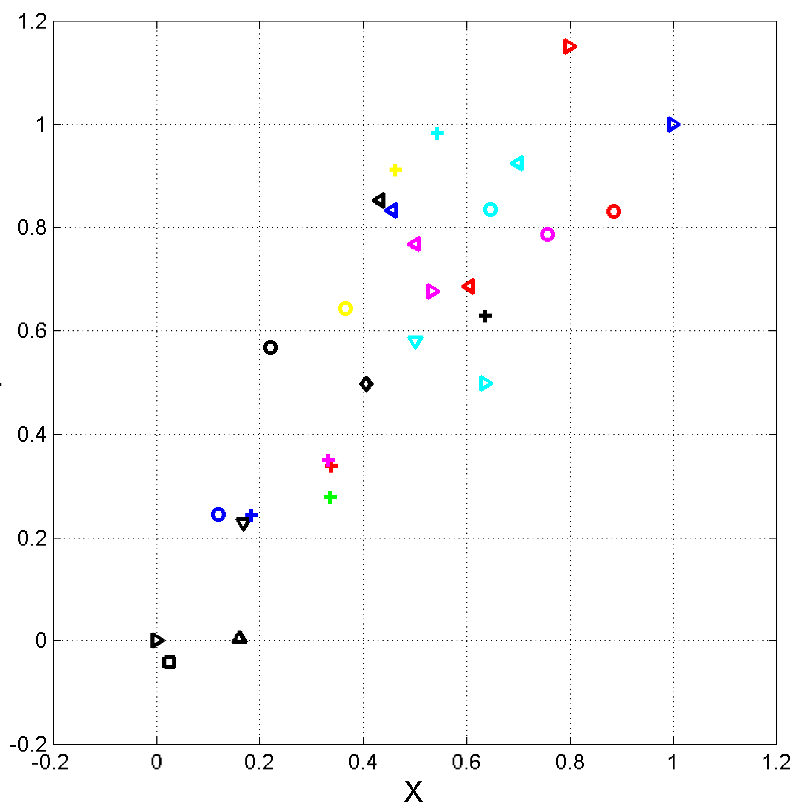
Figure 2.
Greek–1. Averae calculated by considering the input author (left panel, average of the values reported in the corresponding column of Table 5) or the output author (right panel, average of the values reported in the corresponding row). S–Channel: red line; I–channel: blue line; WI–channel: magenta line; I–Channel: green line. Aeneas Tactitian 1; Aeschines 2; Aristides 3; Aristotle 4; Demosthenes 5; Flavius Josephus 6; Herodotus 7; Pausanias 8; Plato 9; Plutarch 10; Polybius 11; Strabo 12; Thucydides 13; Xenophon 14.
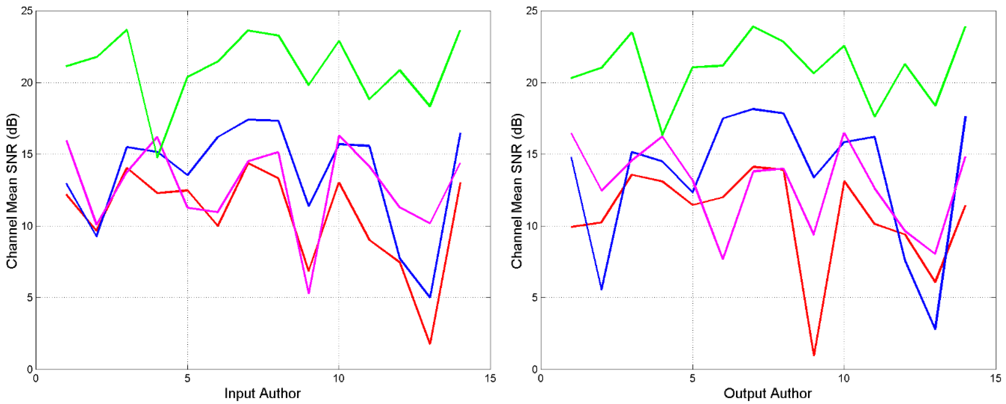
Figure 3.
Greek–2. Average calculated by considering the input author (left panel) or the output author (right panel)). S–Channel: red line; I–channel: blue line; WI–channel: magenta line; I–Channel: green line. Aeschylus 1; Aesop 2; Euripides 3; Iliad 4; Odissey 5; Pindarus 6; Sofocles 7.
Figure 3.
Greek–2. Average calculated by considering the input author (left panel) or the output author (right panel)). S–Channel: red line; I–channel: blue line; WI–channel: magenta line; I–Channel: green line. Aeschylus 1; Aesop 2; Euripides 3; Iliad 4; Odissey 5; Pindarus 6; Sofocles 7.
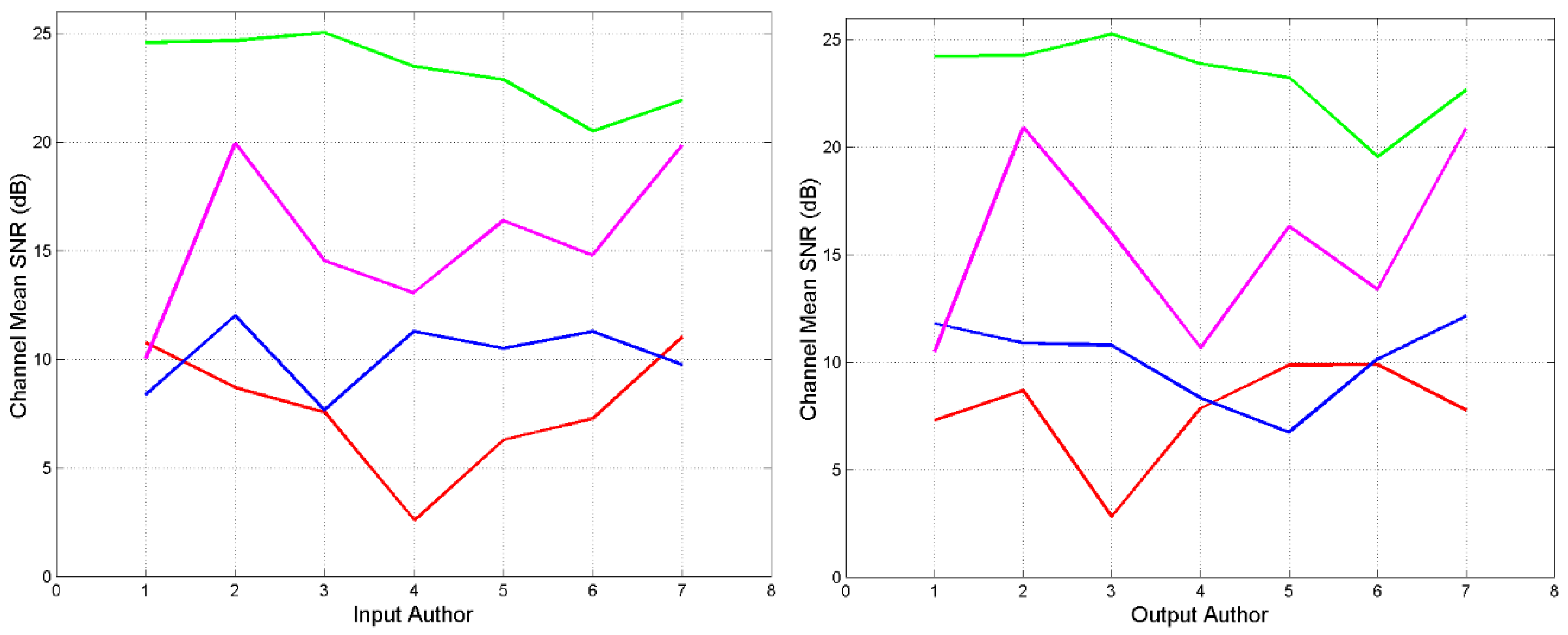
Figure 4.
Left panel: versus in passing from “very difficult” to “difficult” to read. Greek–1: blue circles; Greek–2: cyan circles; NT: red circles. Right panel: , versus distance from the origin (0,0) in the vector plane (Figure 1). Greek–1: blue circles; Greek–2: cyan circles; NT: red circles. The “outlier” text is due to Odyssey.
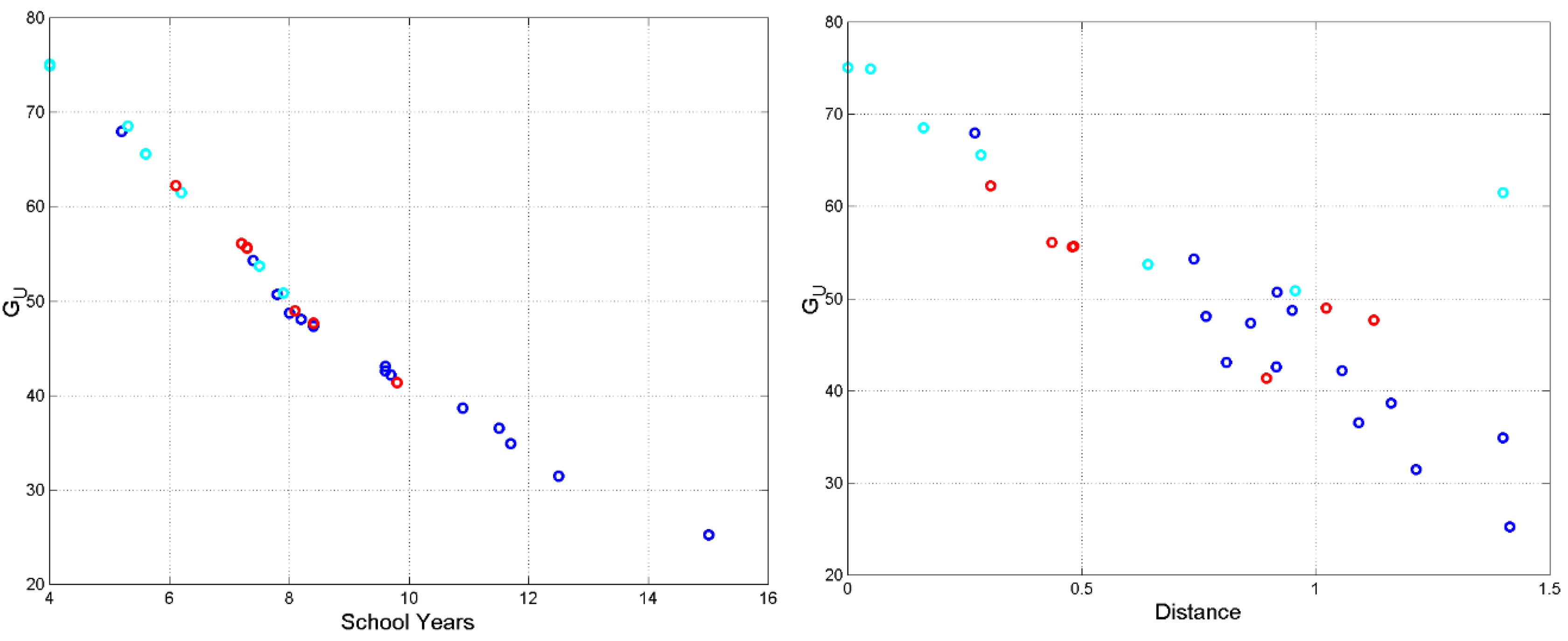
Figure 5.
Left panel: – passing from “very difficult” to “difficult” – versus , Greek–1: blue circles; Greek–2: cyan circles; NT: red circles. Right panel: versus : Greek–1: blue circles; Greek–2: cyan circles; NT: red circles. The largest is due to Flavius Josephus.
Figure 5.
Left panel: – passing from “very difficult” to “difficult” – versus , Greek–1: blue circles; Greek–2: cyan circles; NT: red circles. Right panel: versus : Greek–1: blue circles; Greek–2: cyan circles; NT: red circles. The largest is due to Flavius Josephus.
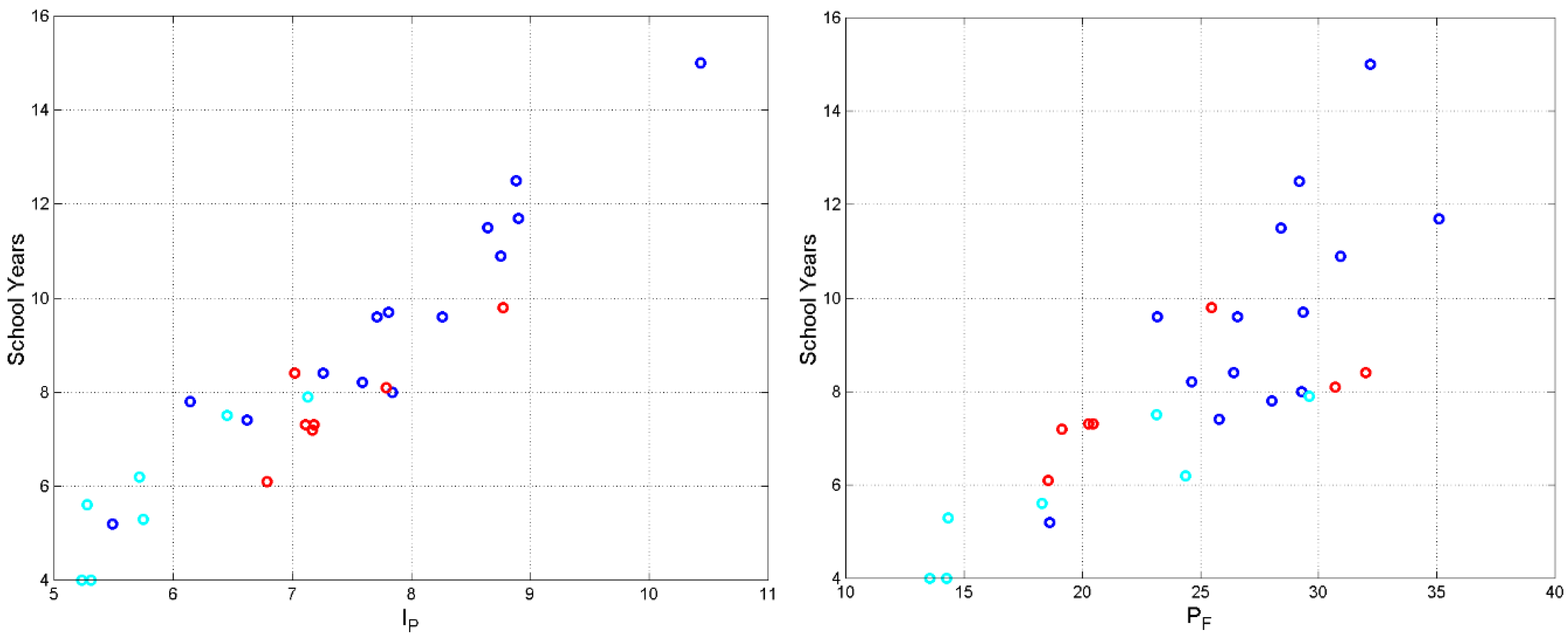
Figure 6.
, versus . The continuous lines are non–linear best fit curves. Greek–1 texts: blue circles and blue line; Greek–2: cyan circles and cyan line; NT: red circles and red line; Italian Literature best fit: green line. English Literature best fit: magenta line [].
Figure 6.
, versus . The continuous lines are non–linear best fit curves. Greek–1 texts: blue circles and blue line; Greek–2: cyan circles and cyan line; NT: red circles and red line; Italian Literature best fit: green line. English Literature best fit: magenta line [].
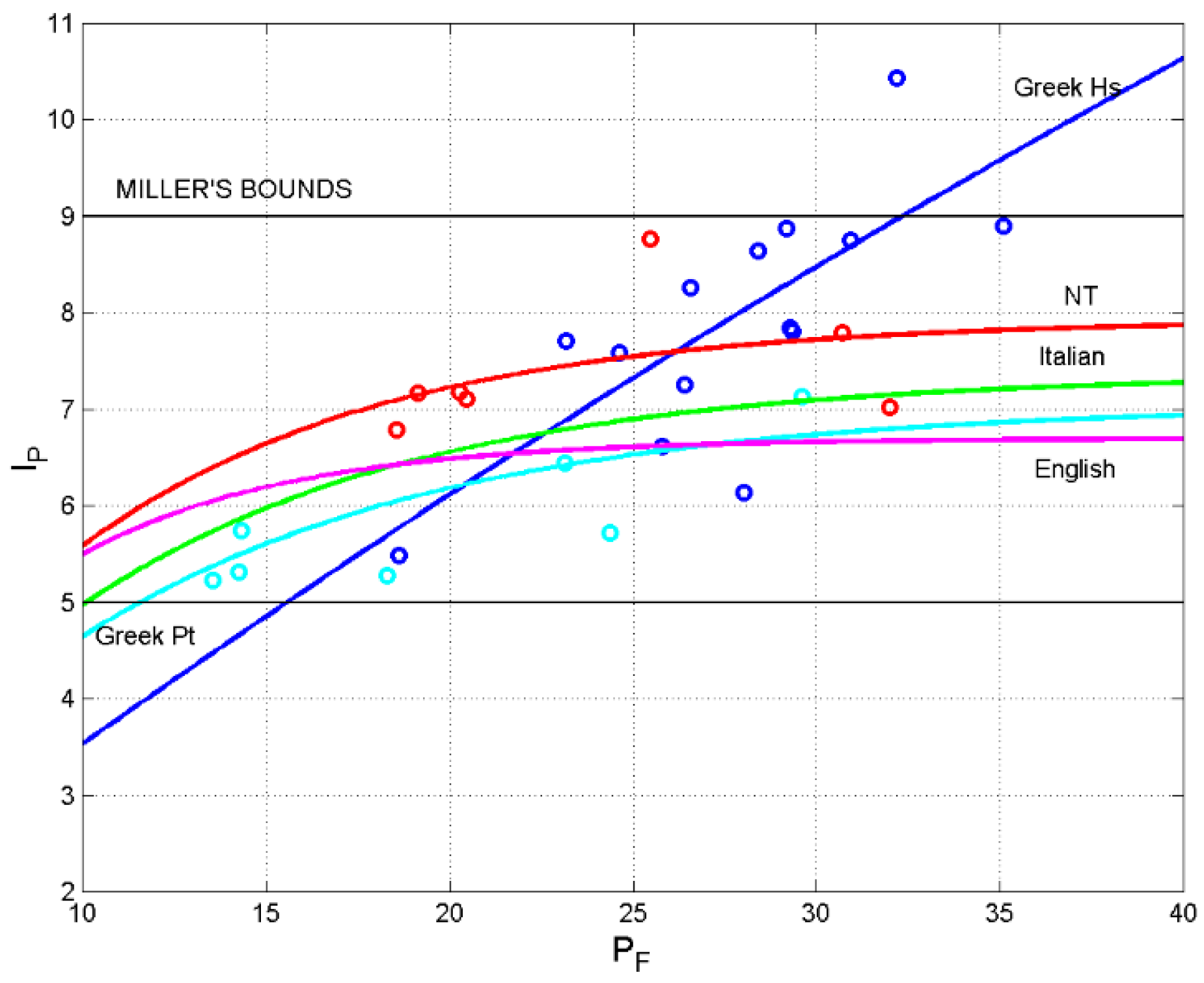
Figure 7.
Scatterplot between and in the Greek Literature (Greek–1 plus Greek–2, blue circles) – this is the entire data samples used to calculate statistical means of Table 3, 4 – and in NT (red circles). The green horizontal line reports the statistical mean ; the black line reports the conditional mean of versus , in 1–unit steps of .
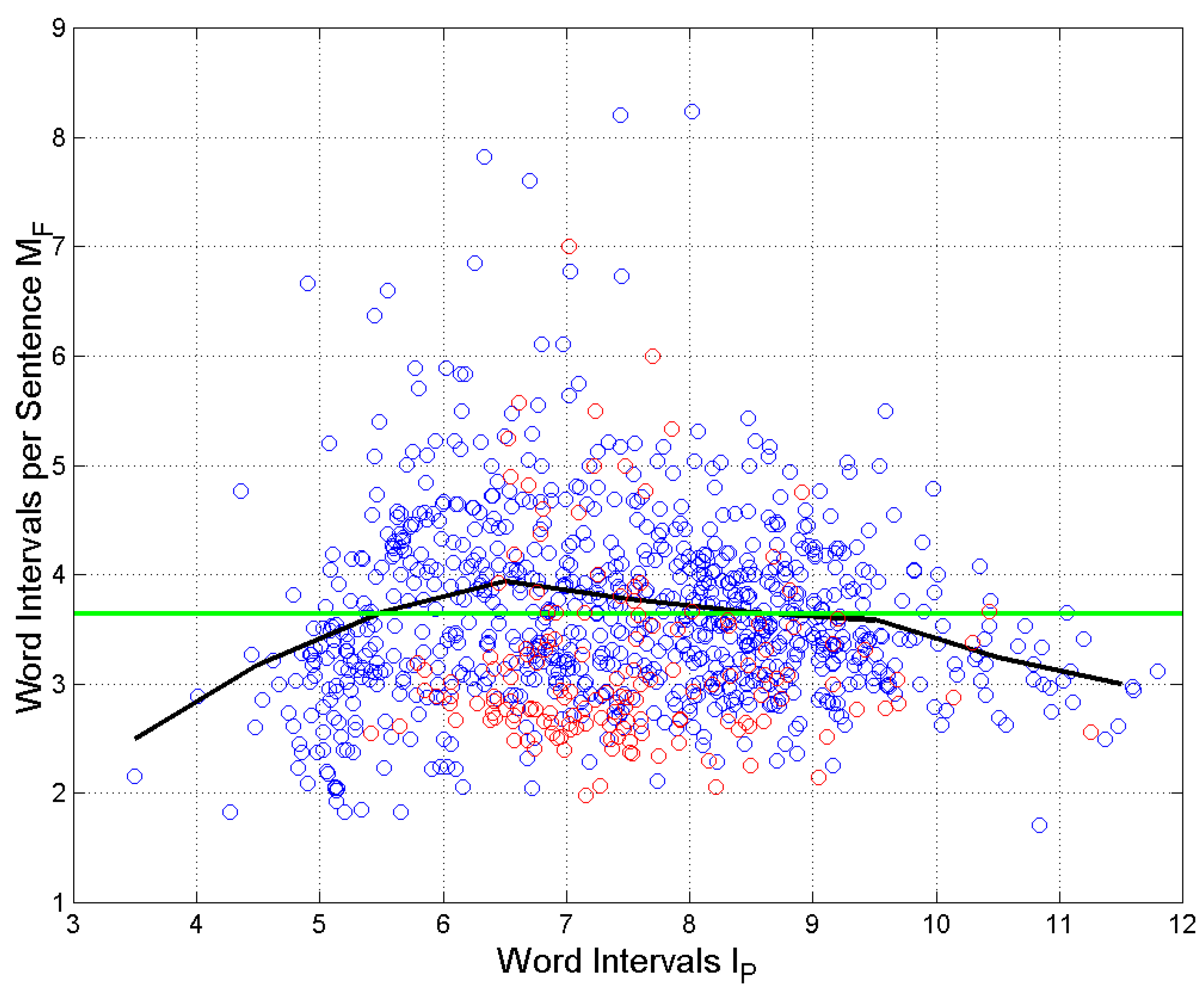
Figure 8.
Probability density of (Left panel) and (Right panel). Greek Literature (Greek–1 plus Greek–2): blue circles; NT books: red circles. The continuous black curves model the Greek Literature samples with a three–parameter log–normal density function.
Figure 8.
Probability density of (Left panel) and (Right panel). Greek Literature (Greek–1 plus Greek–2): blue circles; NT books: red circles. The continuous black curves model the Greek Literature samples with a three–parameter log–normal density function.
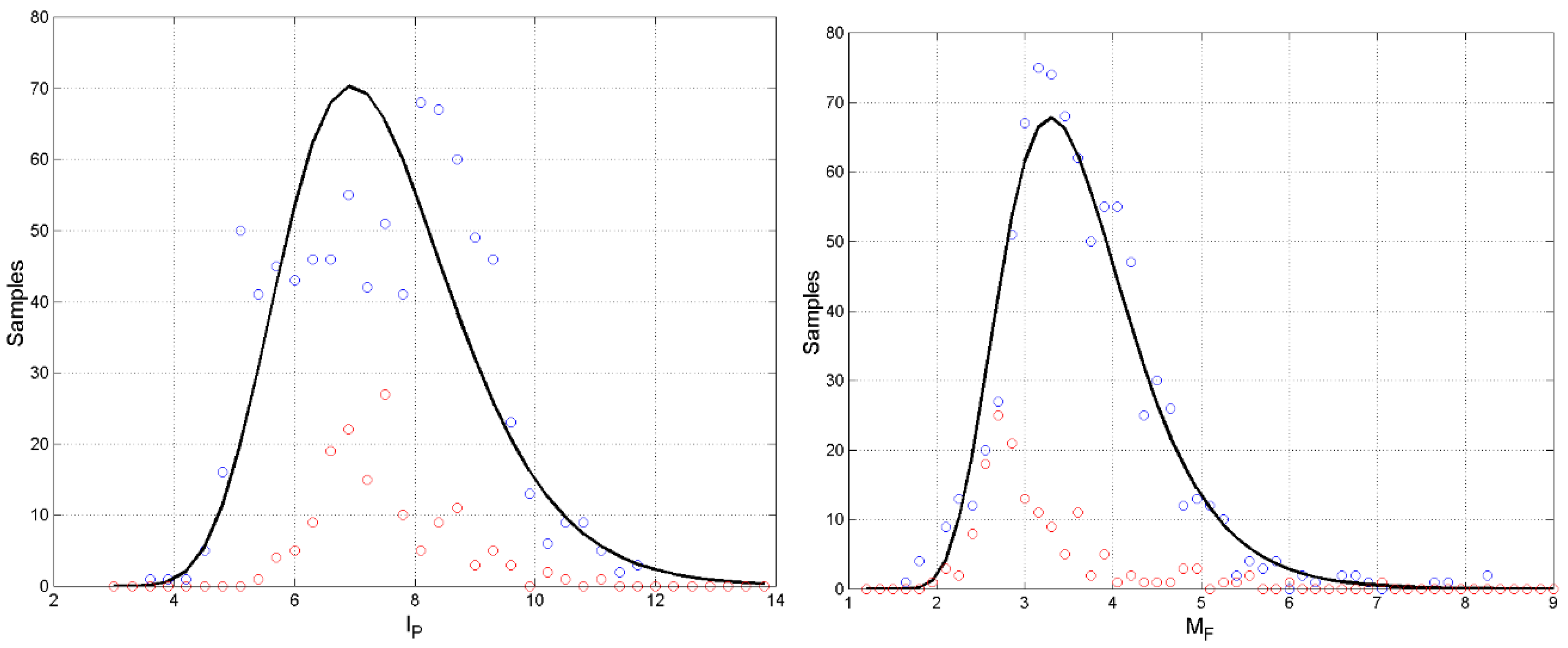
Figure 9.
Left panel: versus (first E–STM buffer). Greek–1: blue circles; Greek–2: cyan circles; NT books: red circles; Italian: green circles; English: black circles. Right panel: scatterplot of versus (E–STM, second buffer). Greek–1: blue circles; Greek–2: cyan circles; NT books: red circles; Italian: green circles; English: black circles.
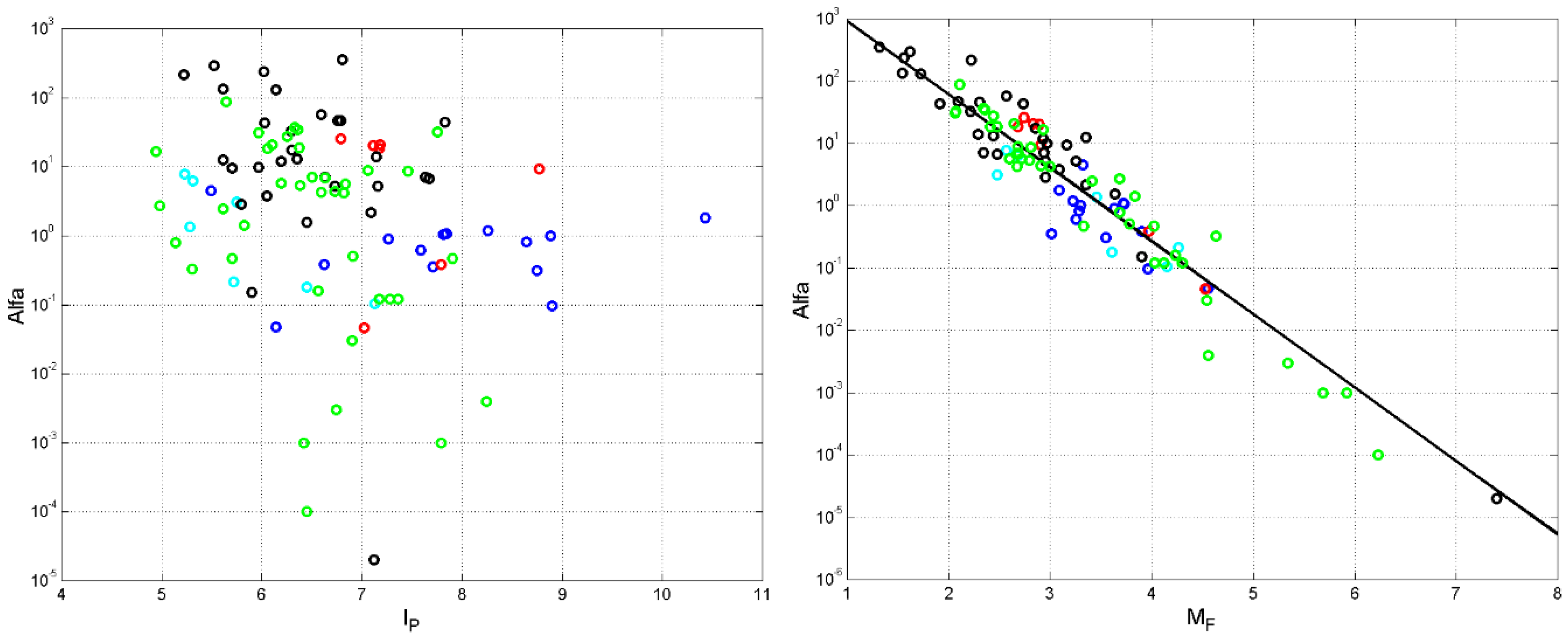
Figure 10.
Left panel: versus . Greek–1: blue circles; Greek–2: cyan circles; NT books: red circles; Italian: green circles; English: black circles. Right panel: scatterplot of versus the mismatch index Greek–1: blue circles; Greek–2: cyan circles; NT books: red circles; Italian: green circles; English: black circles.
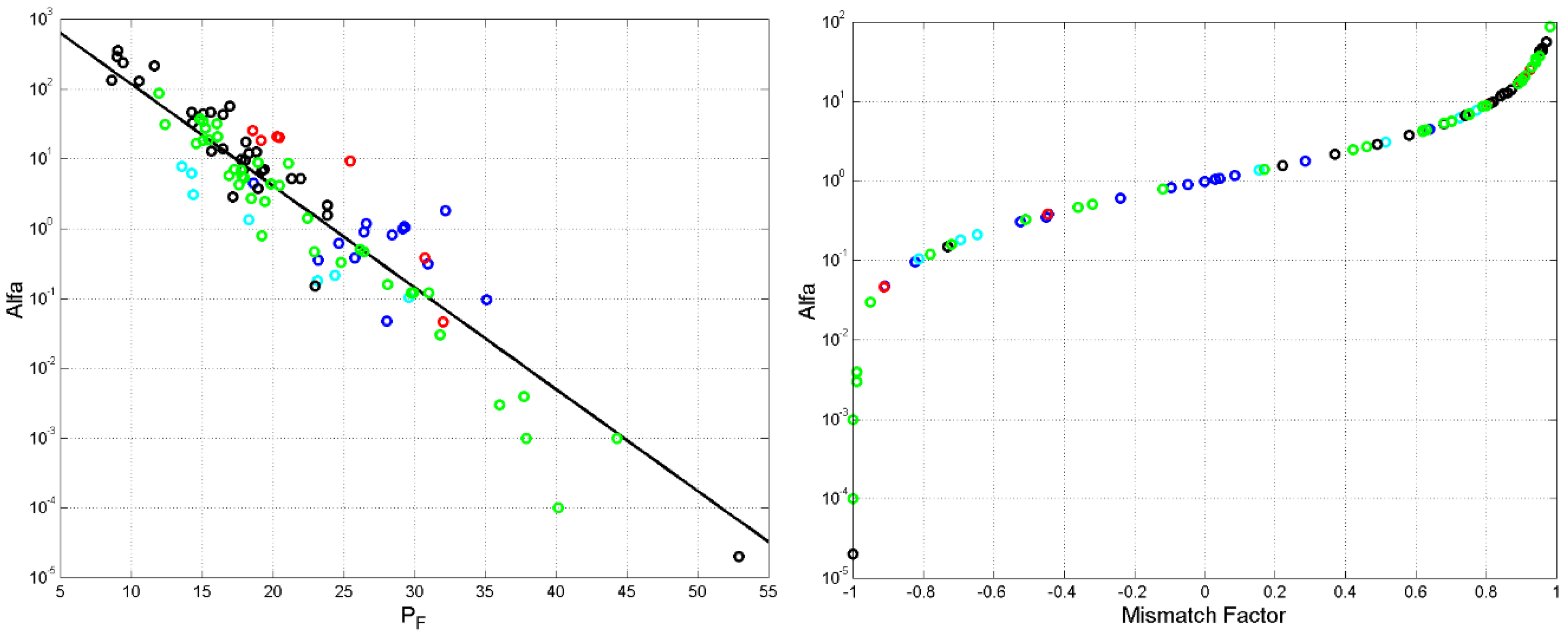
Table 1.
Number of characters, words, sentences and interpunctions contained in the indicated texts of authors belonging to History and other disciplines (Greek–1) and to Poetry and Theatre (Greek–2).
Table 1.
Number of characters, words, sentences and interpunctions contained in the indicated texts of authors belonging to History and other disciplines (Greek–1) and to Poetry and Theatre (Greek–2).
| Texts | Characters | Words | Sentences | Interpunctions | |
|
History and other disciplines (Greek–1) |
|||||
|
Aeneas Tactitian (IV century BC) Military communications |
Poliocertica | 75266 | 13035 | 579 | 1714 |
|
Aeschines (389–314 BC) Statesman, orator |
Against Ctesiphon, Against Timarchus,On the Embassy | 398924 | 69764 | 2555 | 11381 |
|
Aristides (530–462 BC) Statesman, orator |
Orationes | 1205412 | 222272 | 8731 | 30771 |
|
Aristotle (384–322 BC) Philosopher |
De Partibus Animalium, Historia Animalium, Phyisica, Metaphysica, Politica, De Caelo, Politica, Meteorologica, Topica |
2386790 | 509646 | 17790 | 65252 |
|
Demosthenes (384–322 BC) Statesman, orator |
Phylippics 1–4; Adversus Leptinem, In Midiam, Adversus Androtionem, In Aritocratem, In Timocratem, In Aristogitonem 1–2, In Aphobum 1–2, Contra Onetorem 1–2, Olyntiaches | 560697 | 111179 | 4351 | 16812 |
|
Flavius Josephus (37AD–c. 100 AD) Historian |
The Jewish War, Antiquities of the Jews | 2333545 | 424482 | 13272 | 40910 |
|
Herodotus (484–425 BC) Historian and geographer |
Histories 2–9 | 820761 | 157490 | 5945 | 19082 |
|
Pausanias (110–180 AD) Geographer |
Description of Greece 1–10 | 987016 | 176864 | 6272 | 20502 |
|
Plato (428–348 BC) Philosopher |
The Republic, The Apology of Socrates | 547962 | 111125 | 6566 | 20591 |
|
Plutarch (48–125 AD). Historian |
Parallel Lives | 2750711 | 499683 | 17905 | 64365 |
|
Polybius (206–124 BC). Historian |
Histories | 1530968 | 256495 | 8830 | 28997 |
|
Strabo (60 BC–21 AD). Geographer |
Geographica | 821855 | 158993 | 5301 | 18356 |
|
Thucydides (460–404 BC). Historian |
Histories | 814309 | 151906 | 4410 | 17158 |
|
Xenophon (430–354 BC). Historian |
Anabasis | 297161 | 57186 | 2420 | 7634 |
|
Poetry and Theatre (Greek–2) |
|||||
|
Aeschylus (525–456 BC). Playwright |
Agamemnon | 43088 | 8250 | 611 | 1451 |
|
Aesop (620–564 BC). Fabulist |
Fables | 204913 | 39122 | 2172 | 7437 |
|
Euripides (480–406 BC) Playwright |
Medea, Iphigenia in Aulis | 88964 | 17970 | 1392 | 3455 |
|
Homer (IX or VIII century BC) Poet |
Iliad | 548830 | 111878 | 3830 | 15719 |
|
Homer (IX or VIII century BC) Poet |
Odissey | 427148 | 87282 | 3591 | 15259 |
|
Pindarus (518–438 BC) Poet |
Isthmean Odes, Nemean Odes, Olympian Odes, Pythian Odes | 114732 | 21140 | 941 | 3299 |
|
Sofocles (497–406 BC) Playwright |
Electra, Oedipus at Colonus | 95532 | 20077 | 1488 | 3809 |
| All | 17054584 | 3225839 | 118952 | 413954 |
Table 2.
Number of characters, words, words, sentences and interpunctions contained in the indicated books of the New Testament. The genealogies in Matthew (verses 1.1–1.17) and in Luke (verses 3.23–3.38) have been deleted for not biasing the statistical analyses, as in [4,6,7,49].
| Text | Characters | Words | Sentences | Interpunctions |
| Matthew | 88605 | 18121 | 914 | 2546 |
| Mark | 56452 | 11393 | 612 | 1595 |
| Luke | 95180 | 19384 | 964 | 2763 |
| John | 70418 | 15503 | 848 | 2310 |
| Acts | 95647 | 18757 | 760 | 2163 |
| Hebrews | 26317 | 4940 | 164 | 711 |
| Apocalypse | 45970 | 9870 | 333 | 1280 |
Table 3.
Mean values of deep–language parameters , , , in the indicated authors and texts of Greek Literature.
Table 3.
Mean values of deep–language parameters , , , in the indicated authors and texts of Greek Literature.
| > | Years | Multiplicity factor |
Mismatch index |
||||||
| Greek–1 | |||||||||
| Aeneas Tactitian | 5.77 | 23.18 | 7.71 | 3.01 | 43.1 | 9.6 | 0.352 | –0.450 | |
| Aeschines | 5.72 | 28.03 | 6.14 | 4.56 | 50.7 | 7.8 | 0.048 | –0.909 | |
| Aristides | 5.42 | 26.42 | 7.26 | 3.63 | 47.3 | 8.4 | 0.906 | –0.049 | |
| Aristoteles | 4.68 | 29.29 | 7.84 | 3.72 | 48.7 | 8.0 | 1.085 | 0.041 | |
| Demosthenes | 5.04 | 25.80 | 6.62 | 3.90 | 54.3 | 7.4 | 0.384 | –0.445 | |
| Flavius Josephus | 5.50 | 32.17 | 10.43 | 3.09 | 25.2 | 15 | 1.802 | 0.286 | |
| Herodotus | 5.21 | 26.56 | 8.26 | 3.22 | 42.6 | 9.6 | 1.184 | 0.084 | |
| Pausanias | 5.58 | 28.40 | 8.64 | 3.28 | 36.5 | 11.5 | 0.825 | –0.096 | |
| Plato | 4.93 | 18.63 | 5.49 | 3.32 | 68.0 | 5.2 | 4.538 | 0.639 | |
| Plutarch | 5.50 | 29.35 | 7.81 | 3.73 | 42.2 | 9.7 | 1.060 | 0.029 | |
| Polybius | 5.97 | 29.19 | 8.88 | 3.30 | 31.5 | 12.5 | 0.996 | –0.002 | |
| Strabo | 5.17 | 30.94 | 8.75 | 3.55 | 38.7 | 10.9 | 0.311 | –0.525 | |
| Thucytides | 5.36 | 35.10 | 8.90 | 3.96 | 34.9 | 11.7 | 0.097 | –0.823 | |
| Xenophon | 5.20 | 24.62 | 7.59 | 3.25 | 48.1 | 8.2 | 0.612 | –0.241 | |
| Greek–2 | |||||||||
| Aeschylus | 5.22 | 14.34 | 5.75 | 2.48 | 68.5 | 5.3 | 3.117 | 0.514 | |
| Aesop | 5.24 | 18.29 | 5.28 | 3.46 | 65.6 | 5.6 | 1.360 | 0.153 | |
| Euripides | 4.95 | 13.54 | 5.23 | 2.57 | 74.9 | 4.0 | 7.733 | 0.771 | |
| Homer’s Iliad | 4.91 | 29.61 | 7.13 | 4.15 | 50.9 | 7.9 | 0.104 | –0.812 | |
| Homer’s Odissey | 4.89 | 24.37 | 5.72 | 4.26 | 61.5 | 6.2 | 0.214 | –0.647 | |
| Pindarus | 5.43 | 23.13 | 6.45 | 3.61 | 53.7 | 7.5 | 0.180 | –0.694 | |
| Sofocles | 4.76 | 14.26 | 5.31 | 2.68 | 75.1 | 4.0 | 6.279 | 0.725 | |
| All | 5.29 | 28.51 | 8.06 | 3.56 | 42.9 | –– | –– | –– |
Table 4.
Mean values of deep–language parameters , , , in the indicated book of the New Testament.
| Book | > | Years |
Multiplicity factor |
Mismatch index |
|||||
| Matthew | 4.91 | 20.27 | 7.18 | 2.83 | 55.61 | 7.3 | 20.66 | 0.908 | |
| Mark | 4.96 | 19.14 | 7.17 | 2.68 | 56.14 | 7.2 | 18.35 | 0.897 | |
| Luke | 4.91 | 20.47 | 7.11 | 2.89 | 55.68 | 7.3 | 20.21 | 0.906 | |
| John | 4.54 | 18.56 | 6.79 | 2.74 | 62.21 | 6.1 | 25.75 | 0.925 | |
| Acts | 5.10 | 25.47 | 8.77 | 2.91 | 41.35 | 9.8 | 9.41 | 0.808 | |
| Hebrews | 5.33 | 32.00 | 7.02 | 4.53 | 47.71 | 8.4 | 0.05 | –0.912 | |
| Apocalypse | 4.66 | 30.70 | 7.79 | 3.97 | 48.95 | 8.1 | 0.38 | –0.448 |
Table 5.
Greek–1. Average , S–Channel. The author/text in the first row is the reference, i.e. the channel input ; the author/text in the first column is the channel dependent output . For example, if Aristides is the input and Demosthenes is the output, then dB, viceversa, if Demosthenes is the input and Aristides is the output, then dB, a small asymmetry always found in linguistic channels. Cases with dB are highligthed in colour: blue indicates not only that the number of sentences of the input and output texts are signficantly very similar – for the same number of words – but also that the input author might have influenced the output author because he lived before; red indicates a large similarity but no likely influence can be invocated because the input author lived after the output author. Largest : Aristides– Herodotus, dB; minimum : Thucydides–Plato, dB.
| Author | Aeneas | Aeschi | Aristi | Aristo | Demo | Flavius | Hero | Paus | Plato | Plut | Poly | Strabo | Thuc | Xen |
| Aeneas | ∞ | 5.99 | 15.31 | 8.68 | 16.11 | 7.42 | 14.45 | 11.24 | 10.10 | 10.42 | 8.79 | 3.39 | –1.57 | 19.05 |
| Aeschines | 9.18 | ∞ | 8.68 | 15.81 | 7.43 | 8.04 | 9.64 | 10.20 | 5.79 | 15.63 | 4.84 | 18.96 | 7.60 | 11.55 |
| Aristides | 16.69 | 7.75 | ∞ | 11.95 | 23.16 | 12.85 | 27.31 | 18.72 | 7.78 | 13.43 | 14.71 | 5.19 | –0.07 | 16.88 |
| Aristoteles | 11.60 | 16.33 | 13.32 | ∞ | 11.22 | 13.56 | 15.01 | 17.15 | 6.33 | 25.57 | 8.76 | 12.37 | 4.85 | 14.39 |
| Demosthenes | 17.48 | 5.86 | 22.59 | 9.26 | ∞ | 10.32 | 18.44 | 14.07 | 8.35 | 10.56 | 15.00 | 3.49 | –1.48 | 15.02 |
| Flavius | 10.51 | 10.30 | 14.69 | 15.17 | 12.78 | ∞ | 15.63 | 19.09 | 5.76 | 14.27 | 14.35 | 8.55 | 3.14 | 11.63 |
| Herodotus | 15.96 | 8.99 | 27.56 | 13.89 | 19.27 | 14.05 | ∞ | 22.44 | 7.52 | 15.57 | 13.59 | 6.26 | 0.77 | 17.65 |
| Pausanias | 13.39 | 10.64 | 19.74 | 17.05 | 15.68 | 18.06 | 23.12 | ∞ | 6.77 | 17.79 | 13.39 | 7.95 | 2.14 | 15.38 |
| Plato | 6.71 | –1.22 | 3.16 | 0.02 | 4.17 | –0.70 | 2.65 | 1.23 | ∞ | 1.01 | 1.09 | –3.10 | –7.06 | 4.50 |
| Plutarch | 12.84 | 15.26 | 13.98 | 25.08 | 11.74 | 12.24 | 15.84 | 17.03 | 6.83 | ∞ | 8.48 | 10.91 | 3.83 | 16.59 |
| Polybius | 11.67 | 5.82 | 16.21 | 9.20 | 16.51 | 13.00 | 15.03 | 13.93 | 6.59 | 9.81 | ∞ | 3.82 | –1.01 | 11.16 |
| Strabo | 7.69 | 19.97 | 7.47 | 13.26 | 6.39 | 7.54 | 8.28 | 8.95 | 4.99 | 12.58 | 4.28 | ∞ | 11.32 | 9.47 |
| Thucydides | 4.89 | 10.69 | 4.45 | 7.94 | 3.66 | 4.57 | 5.01 | 5.44 | 3.47 | 7.62 | 1.86 | 13.35 | ∞ | 6.06 |
| Xenophon | 19.85 | 9.19 | 15.48 | 12.39 | 13.95 | 8.95 | 16.31 | 13.73 | 8.78 | 15.07 | 8.24 | 6.01 | 0.48 | ∞ |
Table 6.
Greek–2. Average , S–Channel. The author/text in the first row is the reference, i.e. the channel input ; the author/text in the first column is the channel dependent output . Cases with dB (i.e., ) are highligthed in colour: blue indicates not only that the number of sentences of the input and output texts are signficantly very similar – for the same number of words – but also that the input author might have influenced the output author because he lived before; red indicates a large similarity but no likely influence can be invocated because the input author lived after the output author. Largest : Aeschylus – Sofocles, dB; minimum : Iliad–Euripides, dB.
| Author | Aeschylus | Aesop | Euripides | Iliad | Odissey | Pindarus | Sofocles |
| Aeschylus | Inf | 8.04 | 9.75 | –1.70 | 0.73 | 2.48 | 24.49 |
| Aesop | 10.95 | Inf | 8.77 | 4.58 | 7.13 | 9.31 | 11.43 |
| Euripides | 9.41 | 4.43 | Inf | –3.29 | –2.80 | –1.61 | 10.86 |
| Iliad | 5.21 | 8.61 | 4.79 | Inf | 12.54 | 10.71 | 5.36 |
| Odissey | 6.56 | 10.52 | 5.09 | 10.08 | Inf | 20.47 | 6.60 |
| Pindarus | 7.55 | 11.86 | 5.47 | 7.39 | 19.61 | Inf | 7.54 |
| Sofocles | 24.83 | 8.71 | 11.56 | –1.40 | 0.66 | 2.32 | Inf |
Disclaimer/Publisher’s Note: The statements, opinions and data contained in all publications are solely those of the individual author(s) and contributor(s) and not of MDPI and/or the editor(s). MDPI and/or the editor(s) disclaim responsibility for any injury to people or property resulting from any ideas, methods, instructions or products referred to in the content. |
© 2024 by the authors. Licensee MDPI, Basel, Switzerland. This article is an open access article distributed under the terms and conditions of the Creative Commons Attribution (CC BY) license (http://creativecommons.org/licenses/by/4.0/).
Copyright: This open access article is published under a Creative Commons CC BY 4.0 license, which permit the free download, distribution, and reuse, provided that the author and preprint are cited in any reuse.


