
Submitted:
14 January 2025
Posted:
16 January 2025
You are already at the latest version
Abstract
An analytical solution to arbitrarily loaded isotropic rectangular cantilever Kirchhoff plates was presented. In this study the deflection surface was approximated with the sum of a particular solution to the governing differential equation (GDE) and two single series. The terms of the single series were the product of an unknown function of an independent variable and a trigonometric function of the other independent variable, whereby the trigonometric functions were consistent with the deflection-related boundary conditions (zero deflection or not along an edge). On the one hand the terms of the series were required to satisfy the homogeneous GDE, leading to two uncoupled differential equations, one for each unknown function, and so the approximate solution satisfied exactly the GDE. On the other hand the boundary conditions were satisfied only at selected collocation points along the boundary, the number of collocation points in each direction corresponding to the number of terms of the associated series. Numerical results will be presented in a future version of this paper.
Keywords:
Isotropic rectangular cantilever plate
; analytical solution
; two single series
; boundary collocation method
1. Introduction
This paper describes the application of Fogang’s [1] approach based on the boundary collocation method, used for the Kirchhoff plates supported at all corner points whereby the edges are arbitrarily supported (simply supported, clamped or free), to cantilever Kirchhoff plates. The Kirchhoff–Love plate theory (KLPT) was developed in 1888 by Love using assumptions proposed by Kirchhoff [2]. In this study the analysis was conducted using the boundary collocation method. This method, also called the generalized Trefftz [3] approach, consists of the use of trial functions which satisfy the governing differential equations of the problem. The unknown coefficients of those functions are determined by the satisfaction of the boundary conditions at collocation points along the boundary. Many authors worked on analytical methods to plate bending problems but few on cantilever plates. Tian et al. [4] derived analytic bending solutions of rectangular cantilever thin plates subjected to arbitrary loads using the double finite integral transform method; the method overcame the deficiency of the conventional semi-inverse methods. Chen et al. [5] analyzed a general nonlinear flexible rectangular cantilever plate considering large deflection and rotation angle. Hamilton’s principle was applied to obtain the nonlinear differential dynamic equations. Hase et al. [6] emphasized the theoretical study of the integration of multiple point loadings (vertical and Inclined) over the thin cantilever plate to eliminate the twisting and predict the definite bending for the linearly elastic material. Xu et al. [7] introduced the finite integral transform method to explore the accurate bending analysis of orthotropic rectangular thin plates with two adjacent edges free and the others clamped or simply supported: this method eliminated the need to preselect the deflection function, which made it more theoretical for calculating the mechanical responses of the plates. Tohidi et al. [8] investigated circular plate with clamped edges under uniform loading and large deflections by using the point collocation method: large deflection of plate was assumed as a function of small deflection of plate, converting so the problem of a partial differential equation to a system of differential equations that has good convergence rate.
In this paper two single series were considered due to the possibility offered to satisfy the boundary conditions along the four edges, inspired from the Lévy solution that involves one single series and the satisfaction of the boundary conditions along two opposite edges (the other edges are simply supported). Moreover the approach can be seen as a mixed analytical-numerical method: analytical since the efforts and deformations are described analytically throughout the plate and numerical since the boundary conditions are only satisfied at collocation points on the boundary.
2. Materials and Methods
2.2. Governing Equations of the Plate
The Kirchhoff–Love plate theory (KLPT) [1] is used for thin plates whereby shear deformations are not considered. In this section the equations of the KLPT are recalled. The governing equation of the isotropic Kirchhoff plate is given by
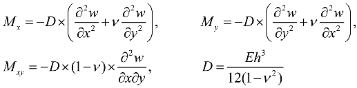
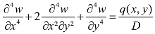 where w(x,y) is the mid-plane displacement in z-direction, q(x,y) the transverse distributed load, and D the flexural rigidity of the plate. The bending moments and twisting moments per unit length Mx and My, and Mxy , respectively, are
The shear forces per unit length are given by
The effective shear forces per unit length used along the free edges are expressed as follows:
In these equations, E is the elastic modulus of the plate material, h is the plate thickness, and ν is the Poisson’s ratio.
2.3. Plate Having Two Adjacent Edges Free and Supported at Three Corner Points
The rectangular plate and the axis convention (X, Y) are represented in figure 1 below.
The plate dimensions in x- and y-direction were denoted by a and b, respectively. The rectangular plate was assumed clamped along the edge x = 0 and free along the other edges.
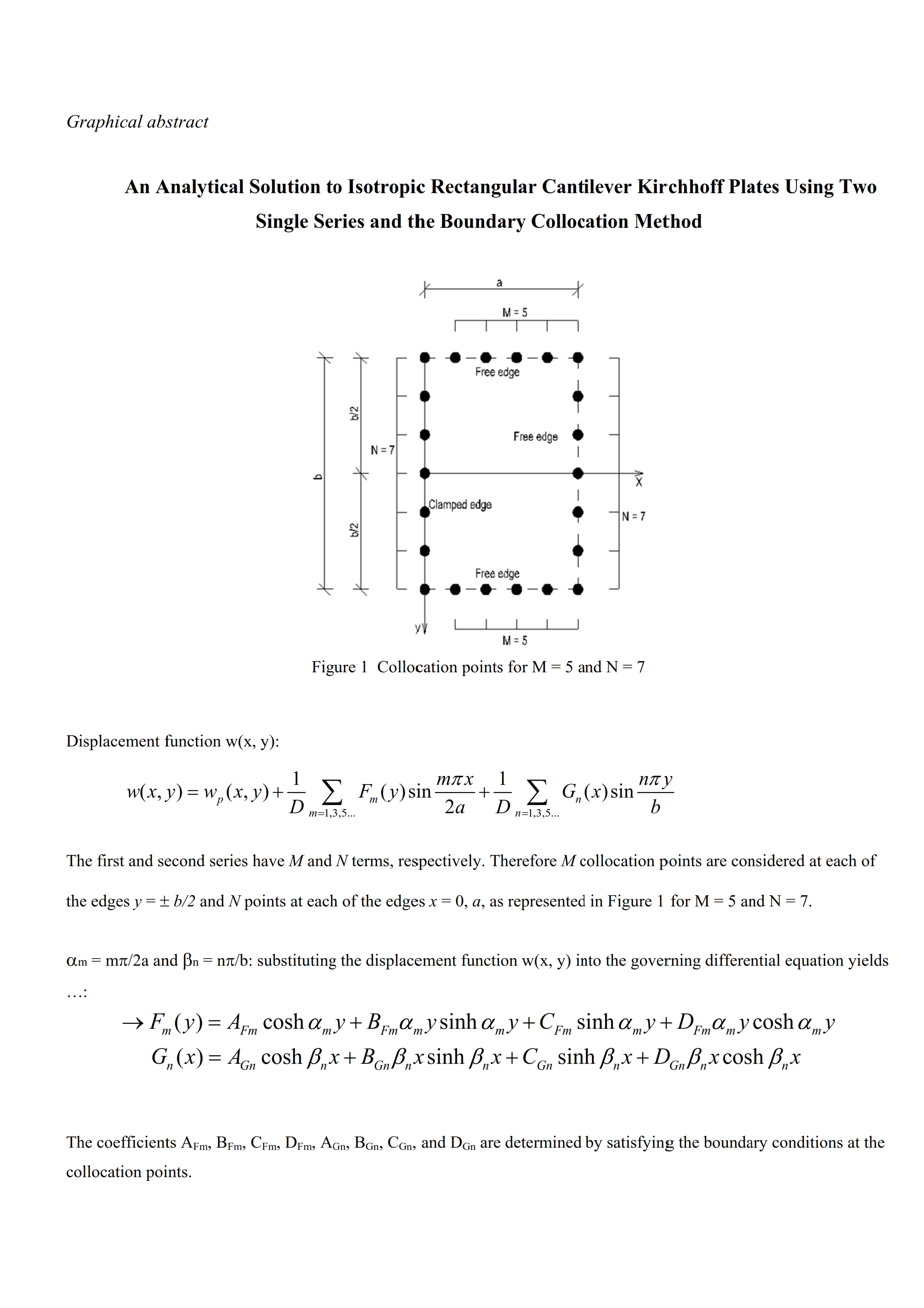
The displacement function was approximated with the sum of a particular solution wp(x,y) to the governing differential equation (1) and two single series. On the one hand the choice of two single series was due to the possibility to satisfy the boundary conditions along the four edges, inspired from the Lévy solution that involves one single series and the satisfaction of the boundary conditions along two opposite edges. On the other hand two single series are "geometrically isotropic," in that the independent variables x and y are treated in the same way in terms of accuracy. The terms of the single series are the product of an unknown function of an independent variable and a trigonometric function of the other independent variable, whereby the trigonometric functions are consistent with the deflection-related boundary conditions (zero deflection or not along an edge). The displacement functions can then be taken
Each of the formulation of Equations (5a-b) can generally be considered. In the following the formulation of Equation (5a) is considered. The term wp(x,y), a particular solution to Equation (1), can be taken as the deflection of a plate strip parallel to the x-axis and subjected to the load q(x,y), and consequently
Setting αm = mπ/2a and βn = nπ/b and substituting Equation (5) into (1) yield
Observing Equation (6) and given that (7) holds for any value of x and y, it results the following differential equations
The solutions to Equations (8a, b) are given by
where the coefficients AFm, BFm, CFm, DFm, AGn, BGn, CGn, and DGn are determined by satisfying the boundary conditions at selected collocation points. The collocation points at the edges x = 0, a are associated with the series having the function Gn(x) while those at y = ± b/2 are associated with the series having the function Fm(y). Let us consider an approximate solution where the first and second series have M and N terms, respectively. It results then 4M + 4N unknown coefficients. Therefore M collocation points should be considered at each of the edges y = ± b/2 and N collocation points at each of the edges x = 0, a, as represented in Figure 2 for M = 5 and N = 7. Since two boundary conditions are set at each collocation point it results in 4M + 4N equations. So there are as many unknowns as equations. It will be shown later that the twisting free condition at the unsupported angles is automatically satisfied by the deflection approximations.
However given the symmetry of the structure, in case of symmetry/anti-symmetry of the loading about the x-axis an appropriate choice can simplify the analysis as follows
- Loading symmetrical about x axis, i.e., q(x, y) = q(x, -y): Equation (5b) is considered for the displacement whereby only the even parts of Fm(y) are considered, leading to CFm = Dfm = 0. The boundary conditions are then applied at only one half of the structure (e.g. y ≥ 0).
- Loading anti-symmetrical about x axis, i.e., q(x, y) = -q(x, -y): Equation (5a) is considered for the displacement whereby only the odd parts of Fm(y) are considered, leading to AFm = Bfm = 0. The boundary conditions are also applied at only one half of the structure (e.g. y ≥ 0).
In case of edge loading the distribution of the collocation points can be taken as represented in Figure 3 for M = 5 and N = 7. It is noted that there is here no point at the plate angles and the collocation points in each direction act over the same length (a/M and b/N).
The bending moments per unit length Mx and My, and the twisting moments per unit length Mxy are expressed using Equations (2a-c), (5), and (9a-b) as follows
The boundary conditions involving the bending moments at the free edges x = a and y = ±b/2 are set observing that for odd values of m and n sin (mπ/2) = (-1)(m-1)/2 and sin (nπ/2) = (-1)(n-1)/2. The twisting moments per unit length Mxy using Equations (2c), (5), and (9a-b) are given by
Given that no twisting should occur at the unsupported angles (a, ±b/2) and observing that the series have zero twisting at these positions (for odd values of m and n cos (mπ/2) = cos (nπ/2) = 0), the particular solution should then be twisting free at these positions.
The effective shear forces per unit length Vx and Vy are expressed using Equations (4a-b), (5), and (9a-b) as follows
The boundary conditions involving the effective shear forces at the free edges x = a and y = ±b/2 are set noting that for odd values of m and n cos (mπ/2) = cos (nπ/2) = 0. The slope ∂w/∂x used as boundary condition is given by
The shear forces Qy used by continuity equations are expressed using Equations (3b), (5), and (9a, b), as follows
The zero deflection condition at x = 0 yields that the constant AGn = 0.
As a recall the coefficients AFm, BFm, CFm, DFm, AGn, BGn, CGn, and DGn are determined by satisfying the boundary conditions at selected collocation points suitably distributed along the plate edges. With increasing number of terms of the series, corresponding to more collocation points, the boundary conditions are better satisfied and consequently the results obtained should converge towards the exact results.
Moreover by applying the boundary conditions the external running moments and running loads should also be suitably distributed at the collocation points.
With the determination of the coefficients above the deflections are calculated using Equations (5) and (9a, b) and the efforts (bending moments Mx, My, and twisting moments Mxy , and effective shear forces Vx and Vy) using Equations (10a-c) and (11a-b).
Analysis of Special Cases
- a)
- Concentrated load acting at unsupported angles
Given a displacement function where the first and second series have M and N terms, respectively. As derived before, the edges x = 0, a and y = ±b/2 are discretized with N and M points, respectively, according to Figure 3. Consequently the grid spacing along the edges x = 0, a and y = ±b/2 are b/N and a/M, respectively. The concentrated force P applied at the unsupported angle can be assumed distributed over the length d = a/M + b/N, and so the boundary conditions involving the effective shear forces, Equations (11a-b), are set as follows
- b)
- Concentrated force and moment applied at the interior of the plate
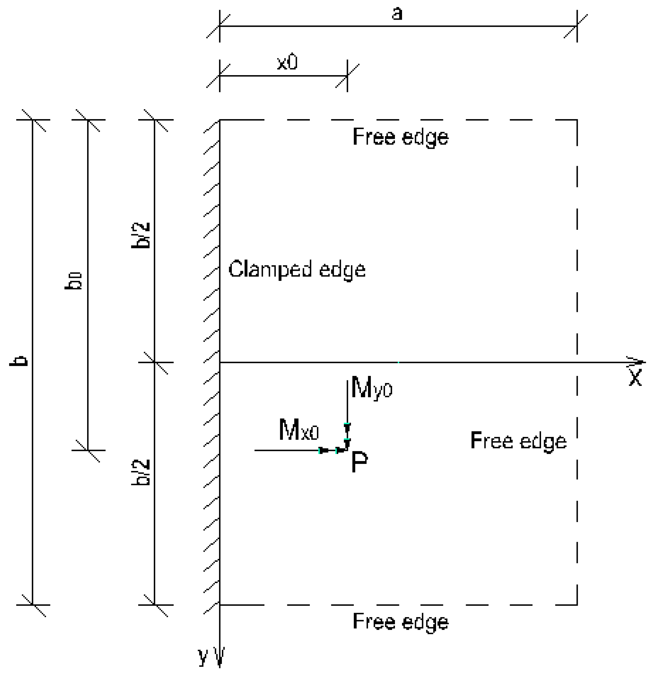
Let an external force P and external concentrated moments Mx0 and My0 be applied at (x0, b0) as shown in Figure 4.
Referring to Figure 4, the deflections defined as before (Equations (5a, b) and (9a, b)) are represented with the subscripts I and II for the plate zones –b/2 ≤ y ≤ –b/2 + b0 and –b/2 + b0 ≤ y ≤ b/2, respectively, as follows
Let the first series of wI and wII have each M terms, and the second series have NI and NII terms, respectively. Therefore, the lines y = –b/2, y = –b/2 + b0, and y = b/2 should be discretized with M nodes, and each of the edges x = 0, a of the plate zone I and II should be discretized with NI and NII nodes, respectively. It results in 4M + 4NI unknowns in plate zone I and 4M + 4NII unknowns in plate zone II, then a total of 8M + 4NI + 4NII unknowns. The external force P and the moments are distributed to the nodes as follows
- If the force P or moment Mx0 is applied at a node the corresponding distributed load p or moment mx0 is obtained by dividing it with the node spacing; otherwise the force or moment is first distributed to the two neighboring nodes and then divided with the grid spacing to obtain the corresponding distributed loads or moments at the nodes.
The continuity equations along the line y = -b/2 + b0 express the continuity of the deflection w and slope ∂w/∂y and the equilibrium of bending moment myy and shear force Qy: these equations are given by
In case of an external moment My0, the latter is replaced by a couple of forces applied in the neighbor nodes.
Equations (16a-d) are set at each of the M nodes along the line y = -b/2 + b0.
Following number of equations are set for boundary conditions and continuity equations
- Plate zone I: 2NI equations at each of the edges x = 0, a and 2M equations at y = -b/2
- Plate zone II: 2NII equations at each of the edges x = 0, a and 2M equations at y = b/2
- 4M continuity equations at y = -b/2 + b0.
In summary, we have a total of 4NI + 4NII + 8M equations. So there are as many unknowns as equations.
It is noted that discrete supports along the line y = -b/2 + b0 can also be modeled. In this case a node is placed at the position of the support and the continuity equation involving the shear force is replaced with a zero deflection equation.
3. Results and Discussion
3.1. Cantilever Plate Subjected to an Anti-Symmetrical Surface Loading p(x, y) = 2py/b
The deflection surface using the symmetry considerations (AFm = Bfm = 0) mentioned earlier is given by
The particular solution is taken as the sum of the deflection of a cantilever plate strip parallel to x-axis and subjected to the anti-symmetrical loading and an additional term such as to be twisting free at the unsupported angles. The node distribution can be taken according to Figure 2 or Figure 3 whereby only one half of the structure is considered. The boundary conditions are set at the edges x = 0, a, and y = b/2. Details of the analysis and results will be presented in a future version of this paper.
3.2. Cantilever Plate Subjected to an Anti-Symmetrical Line Loading p(y) = 2py/b Along x = a
The displacement function using the symmetry considerations (AFm = Bfm = 0) is given by
The node distribution can be taken according to Figure 3 (no node at the unsupported angles) whereby only one half of the structure is considered. The boundary conditions are set at the edges x = 0, a, and y = b/2. Details of the analysis and results will be presented in a future version of this paper.
3.3. Cantilever Plate Subjected to a Uniform Surface Loading p
The displacement function using the symmetry considerations (CFm = Dfm = 0) is given by
The particular solution is taken as the deflection of a cantilever plate strip parallel to x-axis and subjected to the uniform loading: it is noted that the twisting free condition at the unsupported angles is satisfied. The node distribution can be taken according to Figure 2 or Figure 3 and the boundary conditions are set at the edges x = 0, a, and y = b/2.
3.4. Cantilever Plate Subjected to a Uniform Line Loading p Along the x-Axis
With regard to the symmetry of structure and loading the analysis is conducted at half of the structure. The displacement function is taken
The boundary conditions are set at the edges x = 0, a, and y = 0, b/2. Along y = 0 the slope ∂w/∂y = 0 and the shear force Qy = - p/2.
4. Conclusions
In this paper, arbitrarily loaded rectangular cantilever isotropic Kirchhoff plates were analyzed. The deflection surface was approximated with the sum of a particular solution to the governing differential equation and two single series. The terms of the single series were the product of an unknown function of an independent variable and a trigonometric function of the other independent variable, whereby the trigonometric functions were consistent with the deflection-related boundary conditions (zero deflection or not along an edge). While the governing differential equation was satisfied throughout the plate the boundary conditions were only satisfied at selected collocation points along the boundary. Moreover, the twisting free condition at the unsupported angles was automatically satisfied by the deflection approximations. Numerical examples and results will be presented in a future version of this paper.
Conflicts of Interest
The author declares no conflict of interest.
Appendix A: Efforts and Deformations for the Formulation of Equation (5b)
Given that no twisting should occur at the unsupported angles (a, ±b/2) and observing that the series have zero twisting at these positions (for odd values of m cos (mπ/2) = 0 and for even values of n sin (nπ/2) = 0), the particular solution should then be twisting free at this position.
The shear forces Qy used by continuity equations are expressed using Equations (3b), (5), and (9a, b), as follows
References
- Fogang, V. An Analytical Solution to Rectangular Kirchhoff Plates Supported at All Corner Points Using Two Single Series and the Boundary Collocation Method. Preprints 2024, 2024102244. [CrossRef]
- Kirchhoff, G. Über das Gleichgewicht und die Bewegung einer elastischen Scheibe. J. für die Reine und Angew. Math.; vol. 18, no. 40, pp. 51-88, 1850.
- Trefftz, E. Ein Gegenstück zum Ritzschen Verfahren (An alternative to the Ritz method). Proceedings, 2nd International Congress of Applied Mechanics, Zurich, pp. 131-137, 1926.
- B. Tian, Y. Zhong, R. Li. Analytic bending solutions of rectangular cantilever thin plates. Archives of Civil and Mechanical Engineering, Volume 11, Issue 4, 2011, Pages 1043-1052. [CrossRef]
- L. Chen, S. Cui, H. Jing, W. Zhang. Analysis and modeling of a flexible rectangular cantilever plate. Applied Mathematical Modelling, Volume 78, 2020. [CrossRef]
- Hase. AA, Chang, J. "Multiple Point Loading on Thin Cantilever Rectangular Plate Subjected to Pure Bending." Proceedings of the ASME 2021 30th Conference on Information Storage and Processing Systems. ASME 2021 30th Conference on Information Storage and Processing Systems. Virtual, Online. June 2–3, 2021. V001T02A004. ASME. [CrossRef]
- Q. Xu, Z. Yang, S. Ullah, Z. Jinghui, Y. Gao. Analytical Bending Solutions of Orthotropic Rectangular Thin Plates with Two Adjacent Edges Free and the Others Clamped or Simply Supported Using Finite Integral Transform Method. Advances in Civil Engineering. 2020. [CrossRef]
- Zia Tohidi, R., Babai, H., & Sadeghi, A. (2023). Analysis of Clamped Circular Plates with Large Deflections under Uniform Loading using Point Collocation Method. Advance Researches in Civil Engineering, 5(1), 70-85. [CrossRef]
Figure 1.
Rectangular plate and axis convention X, Y.
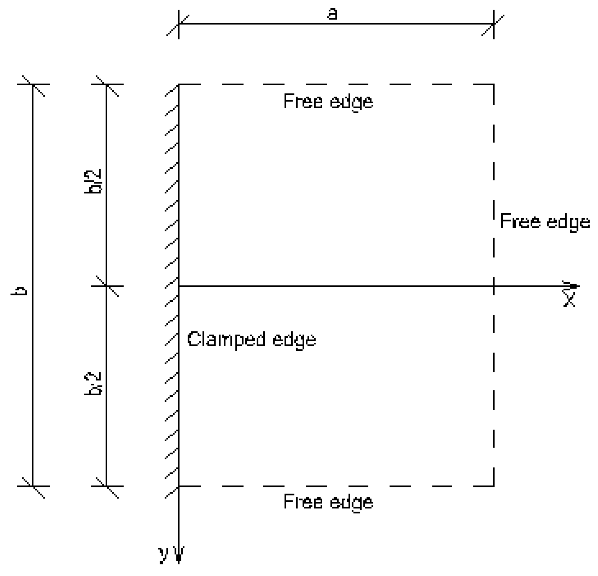
Figure 2.
Collocation points for M = 5 and N = 7.
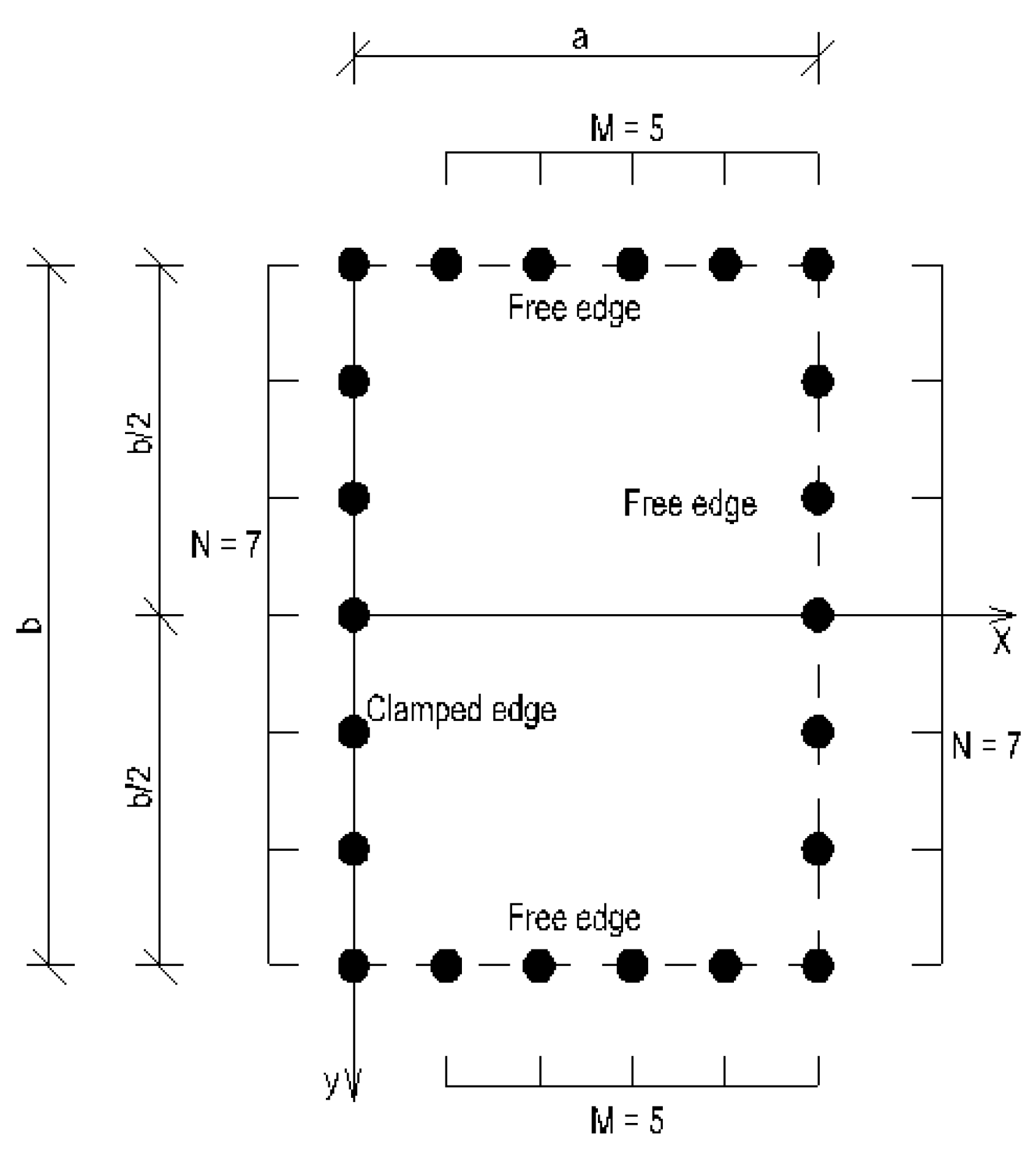
Figure 3.
Collocation points for M = 5 and N = 7 in case of edge loading.
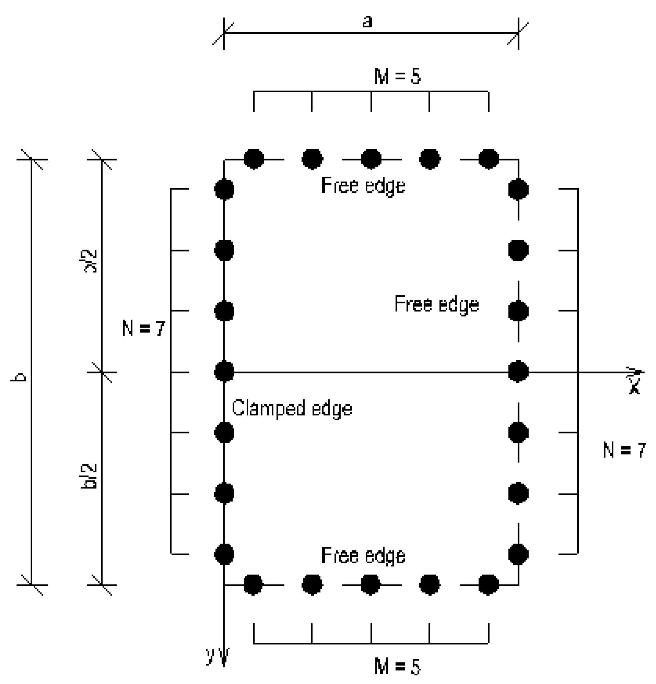
Figure 4.
Plate subjected to an external force P and external moments Mx0 and My0.
Disclaimer/Publisher’s Note: The statements, opinions and data contained in all publications are solely those of the individual author(s) and contributor(s) and not of MDPI and/or the editor(s). MDPI and/or the editor(s) disclaim responsibility for any injury to people or property resulting from any ideas, methods, instructions or products referred to in the content. |
© 2025 by the authors. Licensee MDPI, Basel, Switzerland. This article is an open access article distributed under the terms and conditions of the Creative Commons Attribution (CC BY) license (http://creativecommons.org/licenses/by/4.0/).
Copyright: This open access article is published under a Creative Commons CC BY 4.0 license, which permit the free download, distribution, and reuse, provided that the author and preprint are cited in any reuse.


