
Submitted:
12 November 2024
Posted:
13 November 2024
You are already at the latest version
Abstract
Plastic pollution in waterways poses a significant global challenge, largely stemming from land-based sources and subsequently transported by rivers to marine environments. With a substantial percentage of marine plastic waste originating from land-based sources, comprehending the trajectory and temporal experience of single-use plastic bottles assumes paramount importance. This project designed, developed, and released a plastic pollution tracking device, coinciding with Vietnam's annual Plastic Awareness Month. By mapping the plastic tracker's journey through the Saigon River, this study generated high-fidelity data for comprehensive analysis and bolstered public awareness through regular updates on the Re-Think Plastics Vietnam website. The device, equipped with technologies such as drone flight controller, open-source software, embedded computing, and cellular networking effectively captured GPS position, track, and localized conditions experienced by the plastic bottle tracker on its journey. This amalgamation of data contributes to the understanding of plastic pollution behaviours and serves as a data set for future initiatives aimed at plastic prevention in the ecologically sensitive Mekong Delta. By illuminating the transportation of single-use plastic bottles in the riparian waterways of Ho Chi Minh City and beyond, this study plays a role in collective efforts to understand plastic pollution and preserve aquatic ecosystems.
Keywords:
Plastic Waste
; Riparian Waterways
; Hidden Markov Model
; Extreme Pollution
1. Introduction
This article presents findings on the pressing global challenge of plastic pollution [1], with a focus on the extreme and unique environmental conditions of the Saigon River, part of the greater Mekong River Delta bioregion [2]. A bioregion is a geographic area defined not by political borders but by natural boundaries, such as watersheds, ecosystems, and climatic zones. These regions are characterized by their unique ecological features and biodiversity, often supporting a variety of interconnected species and habitats that form a distinct environmental unit. The Mekong River Delta, known for its vast, biologically diverse wetlands and water systems, plays a critical role in Southeast Asia’s ecology [3]. However, this delicate ecosystem faces significant pressure from plastic waste [4], which threatens not only the biodiversity of the delta but also the livelihoods of communities dependent on its waters.
Drawing upon existing research highlighting that 70 – 80% of marine plastic waste originates from land-based sources, with waterways acting as major transport pathways [3,5], these studies emphasize how rivers serve as major pollution pathways. These Mekong River Delta waterways, often heavily burdened by human activities, act as conveyor belts, carrying massive amounts of plastic waste from urban and industrial centres into marine environments [6]. The Saigon River, as part of this global phenomenon, presents an acute example of this extreme condition [7]. The Saigon River runs through one of the most densely populated and economically active regions of Vietnam, and is inundated with plastic waste, exacerbated by high volumes of industrial discharge and commercial shipping traffic [3,7,8]. These extreme conditions create significant challenges for mitigating plastic pollution and demonstrate the urgency of understanding the movement and impact of plastics through riparian waterways before they reach the ocean [9].
This study emphasizes the extreme conditions within the Saigon River. As a vital artery for Vietnam’s economy, the river is heavily trafficked by commercial shipping, with approximately 2,500 large vessels navigating its waters daily [7,10]. The intense level of human activity, combined with the river's pollution [11], creates a highly challenging and unpredictable environment for any research conducted there. Despite these conditions, the Saigon River serves as a case study for understanding the trajectory and temporal experience of single-use plastic bottles in riparian waterways. The harsh environmental conditions, which include tidal currents, dense shipping traffic, and significant waste and chemical discharge, provide a testing ground for understanding how plastic waste moves through and impacts both the river and its surrounding ecosystems [12]. Through a novel approach, which tracks the journey of a single plastic bottle within these extreme conditions, this research aims to shed light on the broader implications for plastic pollution in sensitive bioregions such as the Mekong Delta, where both ecological and human systems are deeply interconnected.
Further to this, this research highlights a collaboration with Re-Think Plastics Vietnam, a non-governmental organization (NGO) founded in 2018. Their mission is to address the detrimental impacts of plastic pollution by advocating for innovative solutions, conducting research, and actively collaborating with various stakeholders. The organization's approach encompasses public outreach campaigns, engaging educational programs, and community initiatives, all designed to empower individuals and businesses to adopt sustainable practices and reduce their plastic footprint. Through the collaboration with Re-Think Plastics Vietnam, this research supported the NGO's contribution to the ongoing global and localized initiatives in understanding plastic pollution and safeguarding the invaluable aquatic ecosystems of Vietnam.
2. Environmental Context
Movement of plastic in Oceans is well understood. Early approaches have included the use of drift cards [13], to build an understanding of how oceans circulate and rates that plastic pollutants travel [14]. Contemporary research has used oceanographic modelling and ocean current data to predict accumulation and dispersion of plastic pollution from regional coastal areas into the global oceanic system [15]. However, transportation of plastic pollution through urban inland fresh waterways from source to ocean is less understood and is an emerging area of research that combines novel use of technology and single use plastic bottle tracking [12}. Duncan et al., suggest that localized empirical data would enhance current modelling of this global problem [16].
The magnitude and Impact of Plastic Pollution in waterways has emerged as a global environmental crisis [17,18], with rivers acting as significant transport pathways for plastic waste. Studies conducted by Horton et al. [5] reveal that 70-80% of marine plastic waste originates from land-based sources, highlighting the significance of waterways in facilitating the transport of plastic debris to marine environments. In Vietnam, statistics indicate that a substantial amount of plastic waste, ranging from 350g to 7.2kg per capita annually, enters the country's lakes and rivers [19]. Such widespread contamination can have far-reaching consequences for aquatic biodiversity, water quality, and human health.
Studies have also explored the sources and composition of plastic waste in Vietnam's waterways. Research by the Asian Research Centre for Water Resources at the Ho Chi Minh City University of Technology reveals that plastic waste primarily comprises single-use plastic items, including bottles and packaging materials. Furthermore, the study indicates that the Saigon River is contaminated with varying types of plastic pieces, ranging from 10 to 233 pieces per cubic meter [19]. Identifying the sources and types of plastic waste is crucial for designing targeted interventions to mitigate plastic pollution.
Further to this, researchers have introduced a straightforward and adaptable method for quantifying net plastic transport across tidal cycles in a river cross-section, relative to total plastic transport. The researchers employed a Eulerian approach, focusing on a fixed spatial domain to estimate plastic transport by measuring the dynamics of plastic movement and water flow, such as river discharge, flow velocity, and water depths, at sub-hourly intervals. This method was applied to the Saigon River in Vietnam during May 2022, covering six complete tidal cycles [20]. Their findings emphasize the complexity of plastic transport in tidal systems, influenced by factors like changing flow velocities due to tides, the characteristics of plastic items (e.g., buoyancy and rigidity), and interactions with environmental features like riparian vegetation. A key insight is that the net plastic transport is not solely governed by water flow, as other factors like wind and plastic entrapment play a significant role. This complexity is particularly evident in the observation that plastic transport rates can fluctuate between seaward and landward directions due to diurnal tidal cycles [20].
This highlights how understanding the temporal and spatial dynamics of plastic waste transport along waterways is essential for effective waste management strategies. By adopting an approach to track the journey of a single-use plastic beverage bottle along the Saigon River, this research aimed to generate empirical geo spatial data to gain insights into the travel patterns and behaviours of a known pollutant. This data-driven approach could aid in identifying critical areas for waste interception and facilitate informed decision-making.
Plastic pollution in waterways can have detrimental effects on aquatic ecosystems and human health. Studies have demonstrated that plastic debris poses risks to aquatic organisms, leading to entanglement, ingestion, and disruptions in ecosystem functioning. Additionally, microplastics, resulting from the breakdown of larger plastic items, can contaminate water sources and enter the food chain, potentially affecting human health [21]. Understanding the ecological and health implications of plastic pollution is essential for formulating policies and practices to safeguard water quality and biodiversity.
This highlights the pressing issue of plastic pollution in Vietnam's waterways, with severe consequences for aquatic ecosystems and human well-being. A significant percentage of plastic waste originating from land-based sources underscores the importance of effective waste management and prevention strategies. Research on the temporal and spatial dynamics of plastic debris transport could inform targeted interventions to intercept plastic waste before it reaches marine environments. Plastic pollution continues to pose a formidable environmental challenge, further research and collaborative efforts are crucial to develop comprehensive solutions to mitigate its detrimental effects on waterways in Vietnam and worldwide.
On a national level Vietnam has developed a National Action Plan for Management of Marine Litter. Resolution No. 36-NQ /TW of October 22, 2018, of the Eighth Conference of the Party Central Committee XII sets out the goal of a 50% reduction in marine plastic litter by 2025, increasing to 75% by 2030. This policy has the aim of becoming a regional leader in minimizing ocean plastic waste. This ambitious goal is aligned with the United Nations Sustainable Development Goals (SDG) 11 and 14. This research directly supported this by collaborating with Re-Think Plastics Vietnam by gathering and publicizing high fidelity empirical data of the journey of a single use plastic bottle through the riparian waterways of the Saigon River.
The Saigon River is a historically significant waterway in the Mekong delta region and specifically Ho Chi Minh City, Vietnam, flowing through southern Vietnam for approximately 256 kilometers before reaching the East Sea. Its strategic location and navigability have attracted human settlements for millennia, with evidence suggesting that people have been living along its banks for over 3,500 years. With a population of over 9 million people, Ho Chi Minh City heavily relies on the bustling port of the Saigon River for economic activities. The Saigon Port is a network of ports in Ho Chi Minh City [7]. It is the main port of Vietnam and the only one able to host post-Panamax ships.
The river facilitates extensive imports and exports that contribute significantly to the city's GDP, which amounted to $223 billion in 2021 [22]. The rivers historical importance and pivotal role in trade have shaped the region's development over thousands of years, making it an essential lifeline for the people and economy of Ho Chi Minh City. However, the river's environment poses substantial challenges for a device such as a bottle tracker to be placed into. The intense shipping and commercial activities result in approximately 2,500 large commercial vessels navigating the river daily, creating a congested and dynamic waterway [7,10]. The constant traffic of vessels and the tidal water conditions make it a challenging environment for a bottle tracker to navigate effectively [20].
Moreover, the Saigon River faces significant pollution issues, with an estimated 350,000 cubic meters of wastewater discharged into the river annually. The presence of pollutants, including plastic waste and toxic chemicals, posed additional obstacles for the bottle tracker, affecting its functionality and reliability [3,7,8]. The combination of high human activity, water traffic, and pollution renders the Saigon River an extreme environment for a bottle tracker to operate in. The device needed to withstand the harsh conditions, navigate through a crowded waterway, endure potential exposure to pollutants, and resist the UV and heat of the atmosphere while providing accurate data on the bottle's trajectory and spatial-temporal experiences.
3. Research Design
This project had four phases that worked in a linear procession. A collaborative interdisciplinary approach was used that had rapid cycles of hardware development, software integration, prototyping and action research.
3.1. Phase One: Ideation
This phase involved an initial scoping of methods used to aggregate data about plastic waste in riparian waterways. Several systems were investigated and ultimately rejected for this research. Among these was the use of terrestrially based cameras with computer vision functionality to identify and collect data on plastic waste as it passes through the waterway. While this system offered the potential for continuous monitoring, it presented several logistical and administrative challenges. The optimal location for such a setup was identified as a bridge spanning the Saigon River. This site was ideal for capturing the flow of plastic waste through a key section of the river. However, the optimal bridge upon inspection was a multi lane, arterial road that also spanned two distinct city wards, which would introduce two different, often opaque, permission structures. Additionally, the use of such infrastructure would require extensive permitting from both local and national authorities, as structures in this region are often considered sensitive sites due to their strategic importance for transportation and security. Furthermore, the socio-technical landscape in Vietnam means that any surveillance equipment, especially at critical infrastructure points like bridges, could potentially be viewed as a security risk. These complexities ultimately led to the decision to reject this method. The use of a drone to survey a specific location as a base line and then do multiple flight operations at the same location was also considered. This approach would involve post flight analysis of the data and only give a localized tally of plastic waste in the waterway.
The use of GPS tags was also reviewed [16]. The enterprise solution used by these researchers was rejected primarily due to cost and the opaque rules, regulations and administrative burden in Vietnam around customs clearances for importing technology into the country. The use of a low fidelity GPS tracker was also considered, however the limited data output and closed source applications available in consumer grade systems was not optimal for this project.
The systems we reviewed all had advantages as well as disqualifying attributes. A hybrid approach of blending some of the significant benefits of these different systems was adopted. We decided to house a drone autopilot and supporting technologies inside a suitable locally sourced plastic bottle and convert it into a bottle tracker. This approach had the key advantage of not requiring any permitting or permissions from authorities and was expedient in that resources were readily available.
3.2. Phase Two: Prototyping
The project underwent a phase of tandem cycles of hard and software prototyping. Iterative prototyping of hardware and feasibility prototypes of software were employed, resulting in functional prototypes that were tested and refined. This phase culminated in the development of a high-fidelity user prototype in the form of a fully functional artifact. Throughout the process, various prototyping methods, including rapid, evolutionary, and incremental approaches, were utilized to test and evaluate design decisions, leading to continuous improvements in the bottle tracker's features and performance. The iterative nature of the prototyping process allowed for continuous feedback and adjustments until the final artifact was deemed ready for production.
In parallel with the physical processes of prototyping, an initial set-up of a data pipeline using industrial 4G cellular connectivity and open-source software was also focused upon to handle the tracking data efficiently.
3.3. Phase Three: Field Testing
A significant component of this research project was the reliability and resilience of the technology. The robustness and water tightness of the bottle tracker was tested in a controlled environment and then introduced into the environment by testing in canals, connected to the Saigon River, for set periods of time. Telemetry, data, and digital pipeline were also tested by dry land field trips around Ho Chi Minh City to establish and map the data linkage between the bottle tracker and the cellular network it was connected to. This process also served as scouting for possible recovery sites. An action research methodology of planning, acting, observing, and reflecting was used to make any adjustments or adaptations to the bottle tracker as the field testing unfolded.
An important finding from this process was the need to ballast the plastic tracker to ensure it had self-righting capability. This design choice was crucial for maintaining the correct orientation, with the GPS and communication antennas pointing towards the sky, allowing for uninterrupted data transmission. The arrangement relied on positive buoyancy with self-righting capability, which ensured that the tracker remained three-quarters submerged while keeping its upper components above water. After multiple prototypes, this design proved to be the most effective, allowing the tracker to float while maintaining stability even in turbulent conditions.
3.4. Phase Four: Plastic Bottle Tracking and Data Collection
The bottle tracker was launched into the Saigon River on September 1st, 2022, and the data from it was collected in real-time. Daily updates and visualization on the whereabouts of the tracker were provided to the Rethink Plastic host website. The location of the tracker was monitored to ensure that it was functional and that if any unforeseen human interventions or incidents took place, such as interactions with large shipping, the bottle tracker could be retrieved from the waterway and repaired, if necessary. The monitoring also ensured that the bottle tracker did not get caught up in one place.
4. Technologies and Development
A key design constraint for this project was the determination from the team that the bottle tracker had to be a common single-use plastic bottle type, because it is one of the most common plastics found in the river [3], and that daily updates of the tracker’s progress was required for the Rethink Plastics website (https://www.rethinkplasticvietnam.com/tracker) in a Vlog format to support Plastics Awareness Month. The assembly and prototyping of the technology, both hardware and software to allow this was conducted in tandem. The hardware and software contained within the plastic tracker required a capable and flexible autopilot controller as it needed to be stable and multifunctional.
A 3Dr Pixhawk autopilot was selected for the project as it was to hand and simple to re image. This device is configurable as a terrestrial rover and is an open-hardware project providing readily available, low-cost, and a fully featured controller. Importantly it has autonomous capabilities. This device has a suite of sensors that were complimented by a UBlox M6 GPS and Compass module.
- MPU6000 as main accel and gyro.
- ST Micro 16-bit gyroscope.
- ST Micro 14-bit accelerometer/compass (magnetometer).
- MEAS barometer.
The Pixhawk autopilot was imaged with the Ardurover v4.2.3 firmware. This is an open-source firmware specifically developed for un-crewed ground and water vehicles and is an autopilot software stack that is part of the open source Ardupilot eco system. This amalgam of hardware and software is very mature and allows stable, sophisticated management of autonomous vehicles. Initially communication was achieved by using a ground control station (GCS) application called Mission Planner hosted on a laptop. This was wirelessly connected to the Pixhawk controller using an opensource radio platform known as a SiK telemetry radio that transmits serial data on 433 MHz with a power level of 100mw. The protocol Mavlink was used to communicate between the GCS and the Pixhawk controller. This is a lightweight messaging protocol used for telemetry communication that is common in drone and robotic systems. This setup was tested and found to be reliable at localized communication but had a considerable downside as data could only be logged remotely in a continuous mode when connected to the GCS or directly onto an SD card in the device.
At the time of this project a new release of an open soured project called Drone Engage became available. This research project adopted this cloud-based software solution for managing drone operations using the Mavlink protocol and 4G cellular networking. This was an exciting development as Vietnam has a robust cellular network that is widespread with excellent coverage in the Saigon region. This offered hi-fidelity telemetry logging and forwarding to a GCS via the internet in real time.
This approach required integration of a Linux based companion computer, in the form of a Raspberry Pi Zero, onto the Pixhawk controller. Once configured, the software image hosted on the companion computer communicated with the Drone Engage server via Internet using a configured and attached industrial grade 4G dongle, which had up to 150Mbps downlink rate and 50Mbps uplink rate. This embedded computing approach to a telemetry data pipeline was arranged as shown in Figure 1 and Figure 2.
The componentry was housed inside a watertight container that was placed inside the Plastic bottle along with 1.25 kilograms of ballast. This design decision was to give the plastic tracker self-righting abilities, specifically to keep the GPS and Antennas functional. The plastic bottle was made watertight and tested to a hydrostatic pressure of 9.81 kPa for 3 hours in a swimming pool at a depth of one meter. Also, a 13dbi loaded monopole antenna, tuned to 1800 MHz was mechanically fixed to the top of the plastic bottle. Several iterations of the plastic tracker artifact were generated, tested, and refined before a final artifact was produced (see Figure 3 and Figure 4).
5. Data Capture and Processing Approach
The data generated by the plastic tracker was continuously streamed via the cellular link to the drone engage server and accessed by the researchers through the Drone engage web client portal. A web plugin was configured to stream the telemetry data directly, via the internet as a UDP connection, to the mission planner GCS that was set up in Ho Chi Minh City. This telemetry data stream was logged, as Tlog files, which are recordings of the MAVLink telemetry messages sent between the autopilot and the ground station. These files were formatted to generate two key deliverables. The first of these was a data visualization for the daily updates for the Rethink Plastics website during plastic awareness month September 2022 (see Figure 5).
This was achieved by loading 24-hour chunks of the logged data into the Mission Planner GCS simulator while recording the playback. The playback in this environment was manipulated to ensure smooth visualization of the plastic tracker’s movement. This approach resulted in the displayed ground speed data being incorrect but was considered as being appropriate for this application, due to time constraints. Adjustments were made to the simulator settings to reduce any lag or jitter during playback, ensuring that the recorded video captured a clear and continuous path of the tracker. After recording, the video file was introduced into a video editor, where it was significantly sped up to create a more concise and dynamic visualization of the tracker’s journey. This acceleration allowed for the entire journey to be viewed in a format that was engaging and accessible, effectively translating the real-time data into a consumable daily video log for a broader audience.
The second deliverable of this research involved processing and analysing the Tlog telemetry data in 2024. The initial raw data, including GPS coordinates, timestamps, and other relevant metrics, was introduced into the MATLAB software environment.
6. Data Acquisition and Initial Processing
The raw data from the tracker was recorded in the form of Tlog files, which were imported into the MATLAB environment using the UAV Toolbox plugin. This plugin facilitated the conversion of the Tlog data into a more accessible .CSV file format, allowing for subsequent data analysis and manipulation. After the conversion, the data was filtered to retain the most relevant segments.
6.1. Filtering for Activation and Waterway Introduction
We focused on the time-period between the arming of the system, data flow and its introduction into the waterway. This ensured that only data relevant to the bottle’s actual movement through the waterway was retained.
6.2. Timestamp Alignment
To streamline the analysis, the data was further filtered to ensure a consistent time interval of one second between GPS readings. This adjustment facilitated smoother calculations of distance, speed, and other metrics, providing a uniform temporal resolution across the dataset.
6.3. Handling Accelerometer and Compass Data
The plastic bottle tracker was equipped with an accelerometer and a digital compass, which provided additional data on orientation and movement dynamics. However, during the initial analysis, it was observed that the accelerometer data produced conflicting results, likely due to the bottle spinning, rolling, or being subjected to uneven water currents. These variations introduced noise, making it difficult to accurately integrate this data into a smooth analysis of speed and direction.
Additionally, the compass readings were sometimes disrupted, possibly due to rapid changes in orientation or interference from nearby metal objects or environmental factors.
To maintain the integrity of the primary movement analysis, we portioned off the accelerometer and compass data with their corresponding timestamps. By setting this data aside, we ensured that it would not affect the calculations of speed, direction, or distance. This approach also allowed for the possibility of revisiting the accelerometer and compass data for in-depth analysis of specific events or anomalies, such as periods of rapid acceleration or significant changes in orientation.
7. Deriving Additional Metrics
Following the initial processing and filtering, we calculated several derived metrics to enrich the dataset for analysis:
7.1. Speed (m/s)
The speed of the tracker was calculated using the change in distance between consecutive GPS coordinates over each one-second interval. Initial analysis showed that speeds ranged from (0.0 m/s to 0.8 m/s). In instances where consecutive GPS readings indicated the same position, the speed was set to 0 m/s, signifying a resting state.
7.2. Acceleration (m/s²)
Acceleration was derived from the difference in speed values between consecutive time points. This measure indicated periods of increasing or decreasing speed. During periods where the tracker was stationary (resting state), the acceleration values were set to zero to reflect the absence of movement.
7.3. Distance Travelled (m)
The distance between consecutive GPS coordinates was calculated using the Haversine formula within the MATLAB environment, which accounts for the curvature of the Earth. This formula was used to accurately measure the distance over small intervals between successive latitude and longitude points (see Figure 6). For periods identified as resting states, the distance travelled was set to zero, indicating no movement.
7.4. Bearing/Heading (Degrees)
The bearing between consecutive GPS coordinates was calculated to determine the direction of movement relative to true north. The formula used for this calculation is shown in Figure 7.
The formula accounts for the difference in longitude between two points and adjusts the resulting angle using trigonometric functions (atan2, sin, cos) to provide an accurate bearing. This calculation was implemented in MATLAB, where bearings were adjusted to fall within a range of 0° to 360°, ensuring consistent directional references. During periods where the tracker was stationary (resting state), the bearing was set to Not a Number (NaN), to reflect the absence of directional movement.
7.5. Turning Angle (Degrees)
The turning angle was calculated as the change in direction between consecutive bearings. This metric indicated the sharpness of directional changes as the tracker moved through the waterway. Turning angles were set to NaN during resting states to account for the absence of directional change when the tracker was stationary. The turning angle calculation was implemented in MATLAB using the formula as shown in Figure 8.
7.6. Resting State Identification
A "Resting state (Boolean: 0/1)" field was introduced to explicitly identify periods of rest (where the speed was zero). A value of 1 indicated that the tracker was stationary, while 0 indicated movement.
A final step of eliminating any NaN values was also undertaken, these were set to zero. The dataset comprises 836,641 entries, each capturing detailed information about the tracker’s movement. This data processing allowed for an understanding of the tracker’s journey through the waterway, providing insights into its speed dynamics, directional behavior, and overall movement patterns. The processed dataset then served as the foundation for further analysis and visualization in MATLAB and other analytical tools.
8. Preliminary Data Analysis
A series of foundational analysis steps were performed to ensure a robust understanding of the dataset and its characteristics. These preliminary steps provided insights into the tracker’s movement behavior.
8.1. Data Summary and Descriptive Statistics
Descriptive statistics were calculated for key variables, including speed, turning angle, and distance travelled. This step involved determining measures such as the mean, median, standard deviation, and range, offering a quantitative overview of the movement data (see Table 1).
This summary provided initial insights into the variability and central tendencies of the tracker’s speed and direction changes over time.
8.2. Data Visualization
Visualizing the dataset enabled the identification of trends and anomalies in the tracker’s movement. A time series plot of speed over time was used to observe fluctuations in the tracker’s velocity (see Figure 9), while a histogram of turning angles helped understand directional patterns (see Figure 10). Additionally, a pie chart representing the proportion of time spent in "resting" versus "transit" states offered a visual breakdown of the tracker’s behavior (see Figure 11).
The speed graph shows the variations in the tracker's velocity throughout its journey. The average speed is around 0.50 m/s, with a median of 0.53 m/s, indicating that the tracker often maintained a consistent pace. However, there is an interesting anomaly where the speed peaks at 2.55 m/s, significantly higher than the average. This peak may suggest an interaction with an external factor, such as being caught in a current or encountering a rapid flow. The standard deviation of 0.21 m/s reflects moderate variability in the speed data.
The turning angle histogram illustrates the distribution of directional changes made by the tracker. The mean turning angle is 174.77 degrees, with a median of 170.80 degrees, indicating that the tracker frequently made sharp or near-complete directional shifts, possibly due to currents or obstacles. The presence of angles ranging from 0 to 360 degrees suggests that the tracker experienced a full range of turns throughout its movement. The standard deviation of 79.81 degrees points to significant variability in the angles, reflecting changes in the tracker's path.
The pie chart of resting versus moving states shows that the tracker spent the majority of its time in motion, with 91.21% of the entries indicating a moving state, compared to 8.79% in a resting state. The relatively small proportion of resting suggests that the tracker was carried consistently by water currents or external forces, with occasional pauses or slow movements possibly corresponding to calmer water, temporary obstructions or tidal activity.
8.3. Correlation Analysis
To explore relationships between movement parameters, correlation analysis was conducted between speed, distance travelled, and turning angle. The correlation between speed and distance travelled was 0.33, indicating a weak positive relationship. This suggests that as the tracker’s speed increases, the distance between recorded points tends to increase slightly, though the relationship is not strong. This weak correlation may reflect the influence of external factors, such as varying water currents, which impact the distance traveled independently of the tracker's speed.
Similarly, the correlation between speed and turning angle was 0.12, showing a very weak positive relationship. This indicates that changes in speed are only minimally associated with changes in direction. The low correlation suggests that directional changes of the tracker are largely independent of its speed, likely due to external environmental conditions like eddies, currents, or obstacles that alter the path without a direct connection to speed.
This suggests complexity in the tracker's movement through the waterway, where speed and directional changes were influenced by a variety of external factors. These relationships provide a foundational understanding that supports the use of Hidden Markov Models (HMMs) to capture more subtle movement states, such as transitions between resting and transit behaviours.
8.4. Time Series Analysis
Given the time-dependent nature of the data, time series analysis was performed to identify patterns and trends. Autocorrelation plots of speed and turning angle helped assess if there were recurring patterns over time, potentially indicating regular behavior or cyclic movements. This analysis also aided in identifying trends, such as gradual increases or decreases in speed, which could be important for defining movement states.
8.5. Autocorrelation of Speed
The analysis revealed that speed had a moderate autocorrelation at a lag of 3 with a correlation value of 0.58. This suggests a degree of short-term persistence in the tracker’s speed, likely influenced by momentary currents or consistent flow patterns. However, the autocorrelation decreased beyond this point, indicating that speed was less dependent on earlier values as time progressed. The initial high correlation at lag 1 (value of 1.00) was expected, reflecting a lack of abrupt speed changes over very short intervals.
8.6. Autocorrelation of Turning Angle
The turning angle exhibited a weak autocorrelation at lag 2 with a value of 0.21, suggesting that the direction of movement lost correlation quickly as time progressed. This implies that while the tracker tended to maintain direction over very short periods (as shown by the value of 1.00 at lag 1), it was subject to rapid directional changes shortly thereafter.
8.7. Speed Trend over Time
The speed trend analysis (see Figure 12), with a mean of 0.50 m/s and a standard deviation of 0.16 m/s, indicated that the tracker typically moved at a steady pace.
However, notable speed peaks up to 2.32 m/s suggest occasional bursts of speed. These spikes may correspond to interactions with faster currents or being influenced by external factors like water turbulence or passing objects.
8.8. Turning Angle Trend over Time
The trend in turning angles showed an average of 174.77 degrees with a standard deviation of 14.87 degrees, indicating a general pattern of directional stability with occasional adjustments. The range of turning angles, from 117.55 to 222.28 degrees, suggested that while the tracker often maintained a steady course, it was capable of adjusting to changing conditions in the water.
8.9. Geospatial Analysis
The GPS coordinates in the dataset enabled geospatial analysis of the tracker’s movement. A cumulative distance plot provided insights into the overall distance travelled, while trajectory plots of the GPS path illustrated the spatial route taken by the tracker as shown in Figure 13. This spatial visualization was critical for understanding the horizontal trajectory of the plastic tracker in relation to the waterway.
The tracker covered a total distance of 205,744.51 meters (approximately 205.7 kilometers) throughout its journey. This substantial distance indicates a broad range of movement, potentially influenced by varying currents, winds, or other environmental conditions encountered along the path.
The mean distance travelled between recorded points was 4.90 meters. This suggests that the tracker typically drifted or moved by lesser amounts between each measurement, reflecting a relatively steady progression through the water. The small average interval distance could indicate a slow-moving current or consistent tracking intervals.
The maximum distance recorded between two consecutive points was 767.74 meters. This outlier suggests a period where the tracker experienced a significant speed increase or was influenced by a strong current or external force. Such a spike could be due to sudden environmental changes, interactions with water vehicles, or turbulent water conditions.
8.10. Data Anomaly Detection
Identifying and addressing data anomalies ensured the quality and reliability of the dataset. Speed spikes—instances where speed changed abruptly—were detected and examined, as they could indicate noise or measurement errors. Similarly, GPS outliers, which deviated significantly from the expected path, were identified to ensure that any erroneous data points were considered in the analysis.
The analysis identified 453 instances of speed spikes, with a threshold set at 1.14 m/s. These spikes were predominantly clustered between indices 32,577 and 33,029 in the dataset, suggesting a specific event or interaction during the tracker’s journey. This period of increased speed may be attributed to a scenario where the tracker encountered external forces, such as being caught up in a ship’s wake, leading to a significant acceleration beyond the usual movement patterns.
The analysis revealed 55,440 instances of GPS outliers, concentrated at higher indices, suggesting that these anomalies predominantly occur in the latter stages of the tracker's journey. These outliers may indicate signal interference or irregularities in the GPS data, potentially arising from environmental factors or equipment-related issues. Additionally, 30 distance outliers were identified, with a threshold of 832.88 meters. These outliers are spread throughout the dataset and represent instances where the distance between consecutive GPS readings was unusually high. This could be attributed to abrupt changes in the tracker’s movement or possible errors in the GPS recording process.
8.11. Segmented Analysis of Resting and Transit States
The dataset was further segmented into resting and transit states based on the speed and movement patterns. Comparing average speed, distance, and turning angles between these states helped clarify differences in behaviour during resting and movement periods. Resting State Analysis revealed that the total resting duration was approximately 1225.23 minutes, spread across 73,514 entries. During these periods, the average speed was nearly 0.00 m/s, consistent with the expected behaviour of a stationary state. In contrast, the transit state encompassed around 12,718.78 minutes, with 763,127 entries. The average speed during transit was 0.55 m/s, indicating a slow but steady movement when the tracker was in motion. The total distance travelled during transit was approximately 205,744.51 meters, reflecting the significant coverage achieved during these periods of movement. This segmentation provided an understanding of how the tracker’s behavior shifted between different movement states, setting the stage for more in-depth state classification through HMMs.
9. Further Analysis
The Hidden Markov Model analysis was employed, using the MATLAB software environment, to gain a detailed understanding of the transition dynamics and speed behaviour of the tracker during its journey. The method involved training the HMM using the tracker’s speed data, classifying observations into distinct states, Resting and Transit as shown in Table 2.
The estimated transition matrix revealed a strong tendency for the tracker to remain in the Transit state once it had transitioned, with a probability of 1.0000 for staying in the Transit state. Conversely, there was a 0.3560 probability of moving from a Resting state to a Transit state, suggesting occasional shifts from stationary to active phases. The emission matrix highlighted the tracker’s speed characteristics in each state. In the Resting state, the tracker predominantly exhibited medium speeds (0.7934 probability), with lower likelihoods for both low (0.1275) and high (0.0792) speeds, possibly representing minor movements during rest. When in the Transit state, medium and high speeds were more likely (0.6152 and 0.3684, respectively), indicating a more active phase with sustained or accelerated movement. These findings provided insights into the movement patterns of the tracker, offering understanding of transitions between Resting and Transit phases, as well as the behaviour of the tracker in different movement states.
These results suggest that in the Resting state, the tracker is most likely to maintain medium speeds, while in the Transit state, it is more likely to display a combination of medium and high speeds. The transition matrix shows that once the tracker enters the Transit state, it remains there, which could represent a sustained movement phase.
The transition probabilities between states, as shown in the estimated transition matrix and visualized in the State Transition Diagram (see Figure 14), reveal insights into the dynamics of the system. The matrix indicates a 66.77% probability of remaining in the "Resting" state once it is entered. This suggests that periods of rest are more stable, with a relatively high likelihood of continuation before transitioning to another state. In contrast, there is a 33.23% probability of transitioning from the "Resting" state to the "Transit" state, indicating that while rest is stable, transitions to movement are not uncommon.
A key observation is that once in the "Transit" state, the probability of transitioning back to the "Resting" state is 0%. The model estimates that the "Transit" state is absorbing, with a 100% probability of remaining in transit once entered. This suggests that periods of movement are continuous and do not frequently revert back to rest, which may reflect the nature of the tracker’s environment or conditions during data collection, such as sustained motion or momentum.
The direct connection from "Resting" to "Transit" highlights the possibility of transitioning between these states, while the absence of a direct path from "Transit" back to "Resting" visually reinforces the one-way nature of this transition. This analysis aids in understanding the stability and movement patterns of the system, providing a foundation for further interpretation of the HMM model's behaviour.
This suggests that once movement begins, it tends to persist, potentially indicating external factors or inherent characteristics of the subject being tracked that favour sustained transit over frequent stops.
The resting state analysis revealed that the tracker experienced a total of 78 distinct resting periods throughout its journey, with a combined duration of 187.27 minutes. The average resting duration was approximately 2.40 minutes per rest. Most of these resting events were relatively short, with 77 out of 78 lasting around 0.0167 minutes, suggesting brief pauses during transit, likely due to minor changes in environmental conditions or brief interactions with obstacles in the water.
However, a notable outlier was a significantly prolonged resting event lasting approximately 30 hours. This extended resting period occurred at the end of the tracker’s journey when it contacted land. The duration of this final rest shows that once the tracker reached the shore, it remained in place, likely due to being trapped by terrain or other physical barriers. This change from dynamic river conditions to a static environment on land highlights the impact of physical surroundings on the tracker’s movement. Such a transition could be indicative of how natural elements like tides and riverbanks influenced the tracker’s trajectory until it encountered a new, more stable environment on land.
10. Speed Spike Event Analysis
In the preliminary analysis, a notable speed spike event was identified, suggesting a period of rapid movement or interaction with external forces. To gain an understanding of this phenomenon, we isolated the indices corresponding to the event and incorporated additional gyroscopic and accelerometer data from the tracker autopilot. This provided a view of the tracker's behaviour during the speed spike. A visual representation of the combined data, highlighting the variations in speed, gyroscopic, and accelerometric readings over the entire dataset, is included (see Figure 15).
The analysis of the speed data revealed significant variations during the speed spike event. The maximum speed recorded during this period was 2.55 m/s, indicating a sudden burst of movement. The minimum speed observed was 0.3013 m/s at index 4, representing moments where the tracker nearly came to a stop. Due to potential data gaps or missing values, the mean speed and standard deviation could not be calculated, appearing as NaN values. This highlighted the need for further data cleaning or imputation in subsequent analyses.
The gyroscopic data provided insight into the rotational dynamics of the tracker during this period: The average gyroscopic readings across the three axes (x, y, z) were approximately 3.59, -13.53, and 22.25, respectively. This indicated a consistent rotational bias, particularly along the z-axis. Variability in rotation was most prominent around the x-axis, with a standard deviation of 82.74, followed by 66.55 for the y-axis and 50.06 for the z-axis. This suggested dynamic changes in the tracker’s orientation during the event.
Peaks in gyroscopic readings reached values of 971, 1032, and 541 across the three axes, which supported the possibility of rapid rotational movements such as barrel rolling or pitching. Minimum values like -317, -215, and -140 highlighted sharp changes in rotation in the opposite directions, further indicating sudden movement.
The accelerometer data shed light on the forces acting on the tracker during the speed spike: The averages across the axes were -541.88 for x, 58.60 for y, and 2553.32 for z. These values suggested a downward force on the x-axis, minimal movement along the y-axis, and a strong upward acceleration along the z-axis, potentially due to vertical shifts or gravitational effects. High variability in acceleration (434.95 for x, 275.50 for y, and 1826.34 for z) reflected dynamic changes in the tracker's movement, indicating periods of rapid acceleration and deceleration.
Acceleration peaks of 1961, 2225, and 11873 along the axes indicated intense forces acting on the tracker, aligning with rapid shifts or impact-like interactions. Corresponding minimum values, such as -2663, -2228, and -2128, suggested moments of strong deceleration or sudden directional changes.
The data supported the hypothesis that the tracker experienced rapid and dynamic movement during the speed spike event. The high gyroscopic readings, combined with significant acceleration values, indicated rotational motion, potentially barrel rolling, alongside substantial changes in speed. Peaks and troughs in these readings provided insight into the intensity of the movement, aiding in the reconstruction of the tracker's trajectory and interactions during this segment.
To further understand the context and environment of the speed spike event, we used the corresponding GPS data from the tracker and imported it into Google Earth Pro. This allowed for a precise visualization of the tracker's path during the event, helping to identify the specific location where the speed spike occurred. The analysis revealed that this speed spike event took place in a busy commercial area of the waterway, near two large docks and close to the main channel, suggesting possible influences from nearby marine activities. The following images, Figure 16 and Figure 17 illustrate these observations, providing a geographical and contextual background to the speed spike event.
This image provides a broader geographical context, showing the busy area where the speed spike occurred. The proximity to a large dock and the main channel suggests that the tracker might have been influenced by external factors such as increased marine traffic or water currents, potentially contributing to the sudden speed change.
This close-up view highlights the GPS track's chaotic nature during the speed spike event. The dense clustering of points and erratic path suggests intense activity or interaction with turbulent conditions, further emphasizing the dynamic nature of this part of the tracker's journey.
11. Findings
11.1. Overview of Data Collection and Analysis
The data collection process involved deploying a plastic bottle tracker equipped with GPS and sensors, monitoring the tracker's movement and environmental conditions along its journey through the Saigon River. Initial analysis focused on understanding the tracker's overall behavior, including speed, gyroscopic data, and resting states.
The tracker's movement was generally characterized by low average speeds, reflecting the influence of the tidal nature of the river [3]. The analysis of resting states revealed 78 periods where the tracker remained stationary, with an average resting duration of 2.40 minutes, highlighting how factors like tidal reversals and interactions with riverbanks can temporarily immobilize floating debris. Notably, one prolonged rest occurred at the end of the journey when the tracker settled into a tidal mud bank, demonstrating how plastic waste can become retained in such environments.
During this analysis, a notable speed spike event was identified, prompting a closer examination of this occurrence. The isolated indices of the speed spike were analyzed alongside the newly included gyroscopic and accelerometer data, providing insight into potential external forces or dynamic events, such as a ship's wake, that could explain the sudden change in speed. This analysis suggested that the tracker might have experienced rotational movements, such as a barrel roll, during this period of increased velocity, as indicated by fluctuations in the gyroscopic readings.
11.2. Hidden Markov Model (HMM) Analysis
To further understand the transitions between different movement states of the tracker, an HMM was applied. The analysis revealed two distinct states: "Resting" and "Transit." The transition matrix indicated that the tracker had a 66.7% probability of remaining in the resting state once stationary and a 33.3% chance of transitioning from resting to transit. Interestingly, once in the transit state, the probability of remaining in that state was 100%, suggesting that external forces were required to initiate movement but that continuous flow, likely driven by currents and tides, sustained the transit state.
The HMM results provided valuable insights into the dynamics of plastic transport, especially highlighting how transitions from resting to transit are less likely without significant external influences like tidal shifts or boat wakes. The consistent retention in the resting state also aligns with observed resting periods, suggesting that floating debris can become trapped in particular zones before external forces shift them back into motion.
12. Discussion
In this study, we designed and deployed a GPS enabled tracker to understand the movement of a single use plastic bottle extending prior research [12,13,16,20] within the Saigon River’s urban tidal environment. The tracker was developed to capture detailed movement data, including GPS location, speed and orientation, augmented by gyroscopic and accelerometer readings. Field deployment involved releasing the tracker into the River system during Vietnam’s Plastic Awareness Month to gather data across multiple tidal cycles. The goal was to investigate how tidal dynamics and external factors influence plastic transportation and retention in riparian waterways. This study highlights the larger problem [1,2,3], how will we keep on top of the increasing growth of plastics with serious issues on how we manage even now with the output into the oceans [4,5,6] and accumulation on shorelines [11]. This research builds on data [14], and contributes to marine debris modelling more generally [15], adding information [18,20] and building on prior work identifying threats to the river [19,20]. By analyzing the collected data, this study provided critical insights into the transportation behaviours of plastic waste, highlighting the significant impact of tidal reversals, external disturbances, and localized environmental conditions on plastic movement and retention.
12.1. Slow Movement and Resting States in Tidal Enviroments
The tracker's journey was characterized by low average speeds and prolonged stationary periods, especially in areas influenced by tidal reversals and riverbank interactions [20]. These results align with prior studies that emphasize the capacity of tidal rivers and estuaries to retain plastic waste for extended periods due to reversing flows and obstacles such as mud banks [3,5,7]. The tracker’s final resting place in a tidal mud bank is particularly noteworthy, as it suggests that areas with low net discharge or frequent tidal reversals can serve as effective retention zones for plastic debris [20]. This underscores the complexity of predicting plastic pathways in tidal rivers and highlights the need for future models to account for these retention dynamics.
12.2. External Influences and Speed Spike Event.
A unique speed spike event during the tracker’s journey provided an opportunity to examine the impact of external forces, such as vessel-induced turbulence. The accelerometer and gyroscopic data collected during this event indicated rapid acceleration and rotational movement, likely caused by the tracker being influenced by passing vessels or radical turbulence near the main channel. This finding supports the hypothesis that, in busy waterway areas with high traffic, plastic waste may experience sudden and erratic movements. These movements could complicate predictions of plastic transport, especially in regions where human activities interact with natural hydrodynamics. This rotational behavior, observed in gyroscopic data, highlights the potential for dynamic and unpredictable plastic transport patterns, adding a new dimension to our understanding of how plastic moves in tidal environments.
12.3. Hidden Markov Analysis
The Hidden Markov Model (HMM) analysis further clarified the tracker’s behavior by identifying distinct states of movement and rest. The model showed that the tracker was more likely to remain stationary without significant external disruptions, reinforcing the observation that tidal reversals and low net discharge contribute to long-term retention of plastics in certain zones. The HMM analysis also provided insight into the conditions under which transitions to movement occurred, suggesting that tidal mud banks and other retention areas could serve as “temporary repositories” for plastic waste. This aligns with existing research that highlights the role of estuarine and tidal dynamics in plastic retention and transport [20].
12.4. Pollution Models and Broader Context
These findings have important implications for plastic pollution models, particularly in tidal rivers and estuaries. Traditional models estimating plastic transport [9], often assume a unidirectional flow, but this study demonstrates the need for models that incorporate bidirectional flow, tidal influences, and retention zones. The slow movement, frequent resting states, and eventual resting in a tidal mud bank indicate that tidal rivers may act as semi-permanent repositories for plastic waste [20], with retention dynamics that significantly delay transport to open waters. Applying these insights to global models could help improve predictions of plastic emissions into oceans from tidal rivers and estuarine systems, making them more accurate for these complex environments [18].
12.5. Limitations and Scope of Findings
While this study offers a detailed case study of plastic transport in the Saigon River, it is context-specific, and the findings may not be directly applicable to all tidal rivers without considering their unique hydrodynamic and environmental conditions [12]. Additionally, the tracker design itself posed limitations, such as requiring a specific buoyancy configuration to keep the GPS antenna pointed skyward, which may influence its behavior differently from unmodified plastic waste. The results presented here are best understood as illustrative of potential trends rather than universally applicable findings, though the principles observed can inform broader research in similar tidal environments.
12.6. Contribution to the Field
This research contributes to the growing body of knowledge on plastic transport dynamics by demonstrating a low-cost, field-based approach to studying plastic behavior in tidal rivers. The unique combination of GPS tracking, accelerometer data, and HMM analysis enabled a granular understanding of plastic retention and movement under tidal conditions [16]. Additionally, this study’s focus on a real-world, heavily polluted environment like the Saigon River highlights the need for in-situ observations to complement and improve existing plastic transport models and address the issue of plastic pollution pathways [18].
12.7. Future Research Directions
Future planned research will expand on this study by deploying multiple GPS-enabled trackers across a range of tidal and non-tidal rivers to assess variability in transport dynamics under different environmental conditions [16]. Specific focus will be given to areas of plastic accumulation, such as collection and diversion points along the Saigon River, which could serve as targets for cleanup efforts. Another promising direction is to examine how different types of plastic, varying in buoyancy and rigidity, interact with tidal flows and external forces [19]. By deploying multiple trackers with varying buoyancy characteristics, future studies could refine our understanding of plastic transport in tidal environments, with practical applications for pollution control and waste management in similar waterways.
13. Conclusion
In this study, we investigated the movement and retention dynamics of a plastic tracker in the tidal waters of the Saigon River. We employed a combination of low-cost GPS-enabled tracking, accelerometer and gyroscopic sensors, and Hidden Markov Model (HMM) analysis to understand the tracker's behaviour across different movement states. Our approach allowed for detailed monitoring of speed, resting states, and external influences on the tracker's journey. We found that the tidal nature of the river plays a crucial role in the tracker's slow average speeds and frequent resting periods, and that significant external events, such as interactions with vessels, can cause sudden changes in movement, as demonstrated by a notable speed spike event. Additionally, the HMM analysis revealed the likelihood of transitions between resting and transit states, providing insight into the potential for plastic debris retention in tidal zones.
The findings support the notion that tidal dynamics, along with other environmental factors like riverbank interactions and vessel movements, significantly influence plastic transport and retention in tidal rivers. The study’s observations align with existing research on plastic retention in estuaries, emphasizing the complex interplay between river discharge and tidal cycles. The contribution of this work is threefold: first, it demonstrates the practical application of GPS-enabled tracking for monitoring plastic waste; second, it highlights the importance of considering tidal dynamics in plastic transport models; and third, it provides an understanding of the movement patterns of floating debris using an HMM approach.
Future work could expand on this study by deploying similar trackers in other tidal and non-tidal river systems to evaluate the variability in transport dynamics. Further research could also explore how different types of plastic, with varying buoyancy characteristics, interact with river flows and external forces. Additionally, identifying specific collection and diversion points for plastic waste along the Saigon River could enhance targeted cleanup efforts and pollution mitigation strategies.
In addition, we will disseminate information about the study and findings in formats suitable for general public reading in both English and Vietnamese. We do this to ensure local researchers, students, and non-governmental agencies have access to datasets that directly map and inform how discarded single-use plastic bottle waste moves through the inland waterway of the Saigon River. In this way, we work to foster community engagement, support and effect localized environmental action.
Author Contributions
Conceptualization, P.C. and A.M.; methodology, P.C.; software, P.C.; validation, P.C. and AM.; formal analysis, P.C.; investigation, P,C.; resources, P.C.; data curation, P.C.; writing—original draft preparation, P.C. and A.M.; writing—review and editing, P.C. and A.M.; visualization, P.C.; supervision, A.M.; project administration, P.C. and A.M.; funding acquisition, A.M. and P.C. All authors have read and agreed to the published version of the manuscript.
Funding
This research received no external funding.
Institutional Review Board Statement
Not applicable.
Informed Consent Statement
Not applicable.
Data Availability Statement
The data presented in this study are available on request from the first author. The data is not publicly available due to the costs and resources involved in making the dataset legible enough to be publicly accessible. We will make the data publicly available in the next iteration of this project.
Acknowledgments
The authors acknowledge internal funding support from School of Future Environments (SoFE) and Faculty of Design and Creative Technology (DCT) at Auckland University of Technology (AUT).
Conflicts of Interest
The authors declare no conflicts of interest.
References
- Borrelle, S. B., Ringma, J., Law, K. L., Monnahan, C. C., Lebreton, L., McGivern, A., … & Rochman, C. M. (2020). Predicted growth in plastic waste exceeds efforts to mitigate plastic pollution. Science, 369(6510), 1515-1518. [CrossRef]
- Tran, T. A. (2016). Transboundary mekong river delta (cambodia and vietnam). The Wetland Book, 1-12. [CrossRef]
- Nyanga, C., Njeri Obegi, B., & To Thi Bich, L. (2022). Anthropogenic Activities as a Source of Stress on Species Diversity in the Mekong River Delta. IntechOpen. doi: 10.5772/intechopen.101172.
- Geyer, R., Jambeck, J., & Law, K. L. (2017). Production, use, and fate of all plastics ever made. Science Advances, 3(7). [CrossRef]
- Horton, A. A., Walton, A., Spurgeon, D. J., Lahive, E., & Svendsen, C. (2017). Microplastics in freshwater and terrestrial environments: evaluating the current understanding to identify the knowledge gaps and future research priorities. Science of the total environment, 586, 127-141.
- Lebreton, L., Zwet, J. V. D., Damsteeg, J. W., Slat, B., Andrady, A. L., & Reisser, J. (2017). River plastic emissions to the world’s oceans. Nature Communications, 8(1). [CrossRef]
- Pham, H. T., Ngô, V. T., Pham, T. T., & Bùi, T. T. (2022). The role of mangroves in supporting ports and the shipping industry to reduce emissions and water pollution (Vol. 231).CIFOR. https://pdfs.semanticscholar.org/9ff1/1ff1cef48ef0b7e01dd98b766efff458aa9c.pdf.
- Shinkai, Y., Truc, D. V., Sumi, D., Canh, D., & Kumagai, Y. (2007). Arsenic and other metal contamination of groundwater in the mekong river delta, vietnam. Journal of Health Science, 53(3), 344-346. [CrossRef]
- Emmerik, T. v., González-Fernández, D., Laufkötter, C., Blettler, M. C. M., Lusher, A., Hurley, R.., Ryan, P. G. (2023). Focus on plastics from land to aquatic ecosystems. Environmental Research Letters, 18(4), 040401. [CrossRef]
- Saigonport. (2024, January 8). Vietnam’s ports see over 50,000 vessels in H1. Saigon Port. https://saigonport.vn/vietnams-ports-see-over-50000-vessels-in-h1/.
- Browne, M. A. O., Crump, P., Niven, S. J., Teuten, E. L., Tonkin, A., Galloway, T. S., … & Thompson, R. C. (2011). Accumulation of microplastic on shorelines woldwide: sources and sinks. Environmental Science &Amp; Technology, 45(21), 9175-9179. [CrossRef]
- Newbould, R., Powell, D. M., & Whelan, M. J. (2021). Macroplastic debris transfer in rivers: a travel distance approach. Frontiers in Water, 3. [CrossRef]
- Shannon L V., Stander GH, Campbell JA (James A. Oceanic circulation deduced from plastic drift cards. Department of Industries, Sea Fisheries Branch; 1973. 31 p.
- Pearce, A., Jackson, G., & Cresswell, G. R. (2019). Marine debris pathways across the southern Indian Ocean. Deep Sea Research Part II: Topical Studies in Oceanography, 166, 34-42. https://www.sciencedirect.com/science/article/abs/pii/S0967064517303934?via%3Dihub.
- Critchell K, Grech A, Schlaefer J, Andutta FP, Lambrechts J, Wolanski E, Modelling the fate of marine debris along a complex shoreline: Lessons from the Great Barrier Reef. Estuar Coast Shelf Sci ;167:414 26. https://www.sciencedirect.com/science/article/pii/S0272771415301098.
- Duncan, E. M., Davies, A., Brooks, A., Chowdhury, G. W., Godley, B. J., Jambeck, J., Maddalene, T., Napper, I., Nelms, S. E., Rackstraw, C., & Koldewey, H. (2020). Message in a bottle: Open source technology to track the movement of plastic pollution. PLOS ONE, 15(12), e0242459. [CrossRef]
- Vince, J. (2022). A creeping crisis when an urgent crisis arises: the reprioritization of plastic pollution issues during covid-19. Politics &Amp; Policy, 51(1), 26-40. [CrossRef]
- Winterstetter, A., Grodent, M., Kini, V., Ragaert, K., & Vrancken, K. C. (2021). A review of technological solutions to prevent or reduce marine plastic litter in developing countries. Sustainability, 13(9), 4894. [CrossRef]
- Saigon river threatened by plastic waste. (2019, December 3). Vietnamnet Global. https://vietnamnet.vn/en/saigon-river-threatened-by-plastic-waste-594490.html.
- Schreyers, L. J., Van Emmerik, T. H. M., Bui, T.-K. L., Van Thi, K. L., Vermeulen, B., Nguyen, H.-Q., Wallerstein, N., Uijlenhoet, R., & Van Der Ploeg, M. (2024). River plastic transport affected by tidal dynamics. Hydrology and Earth System Sciences, 28(3), 589–610. [CrossRef]
- Koelmans, A. A., Kooi, M., Law, K. L., & Van Sebille, E. (2017). All is not lost: Deriving a top-down mass budget of plastic at sea. Environmental Research Letters, 12(11), 114028. [CrossRef]
- Vietnam: GDP contribution by province 2021. (2022, June 16). Retrieved from https://www.statista.com/statistics/1326834/vietnam-gdp-contribution-by-province/.
Figure 1.
(Cleveland, 2023) Technology arrangement [diagram]. .
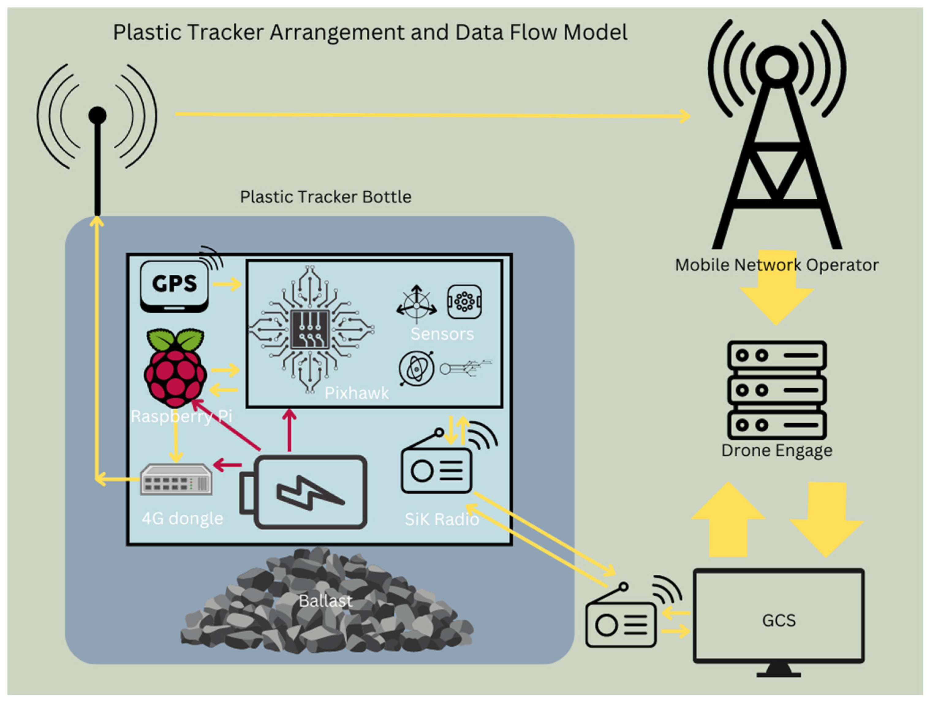
Figure 2.
(Cleveland, 2022) Technology arrangement [photo].
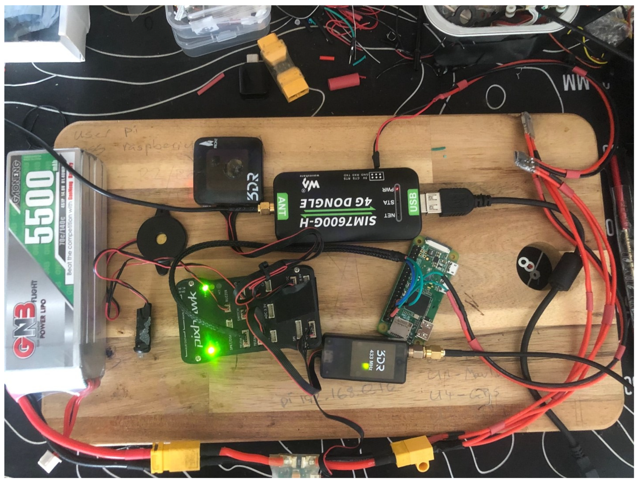
Figure 3.
(Cleveland, 2022) Plastic Tracker Development [photo].
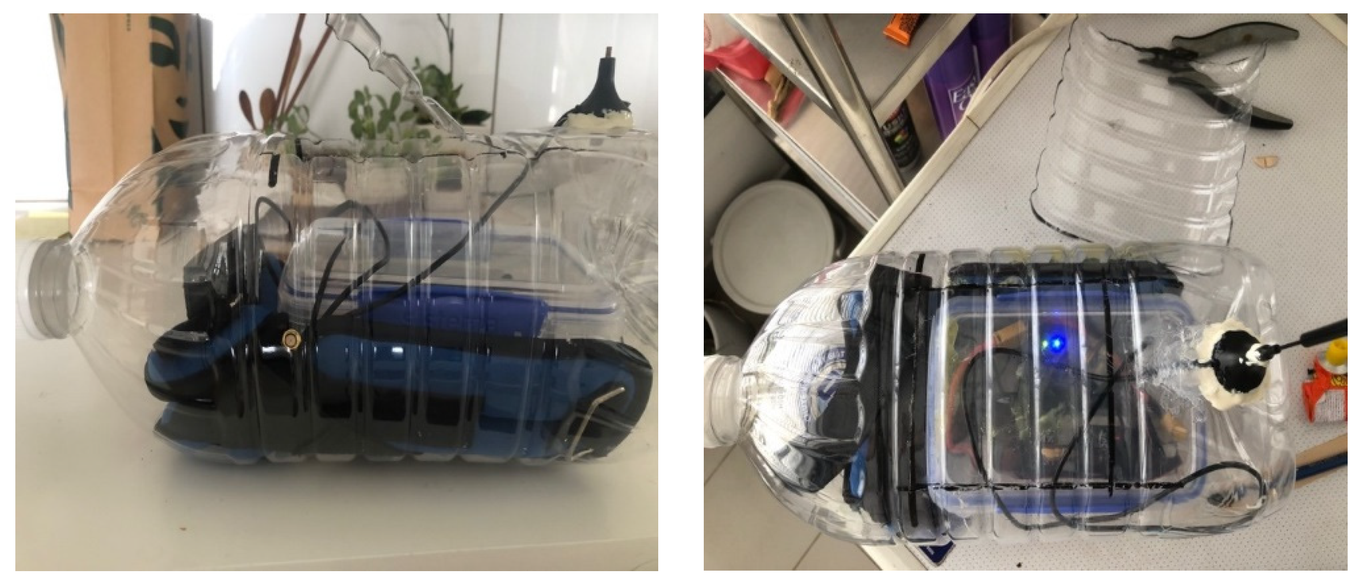
Figure 4.
(Cleveland, 2022) Plastic Tracker final prototype as released into the river [photo].
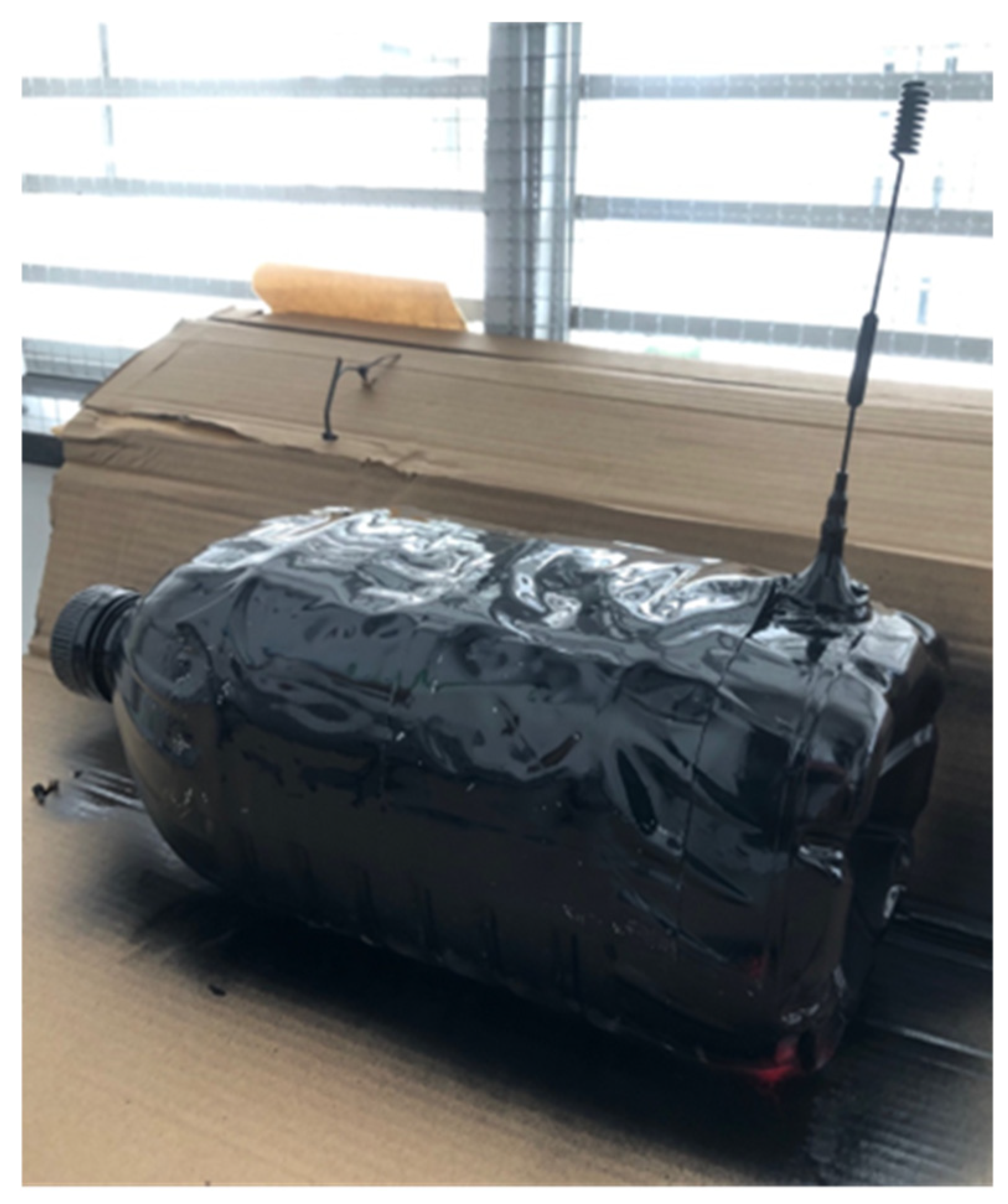
Figure 5.
Day 2 daily update [screenshot].
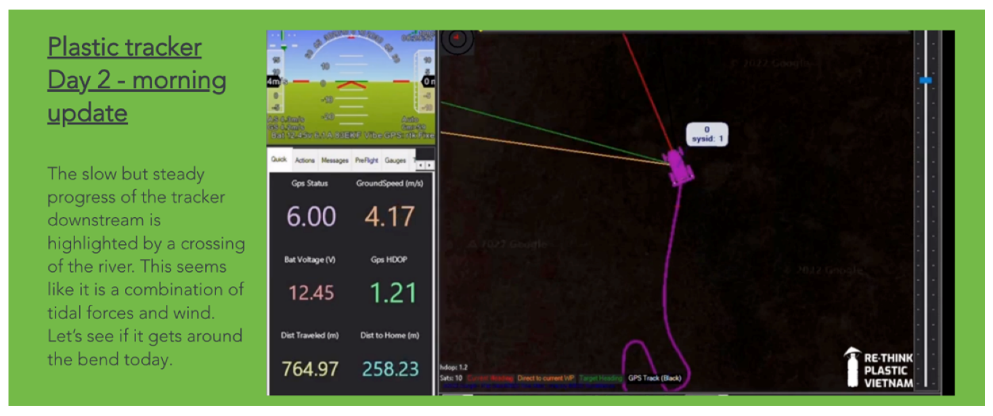
Figure 6.
The Haversine formula used for calculating the distance between two geographical points [Screenshot].
Figure 6.
The Haversine formula used for calculating the distance between two geographical points [Screenshot].
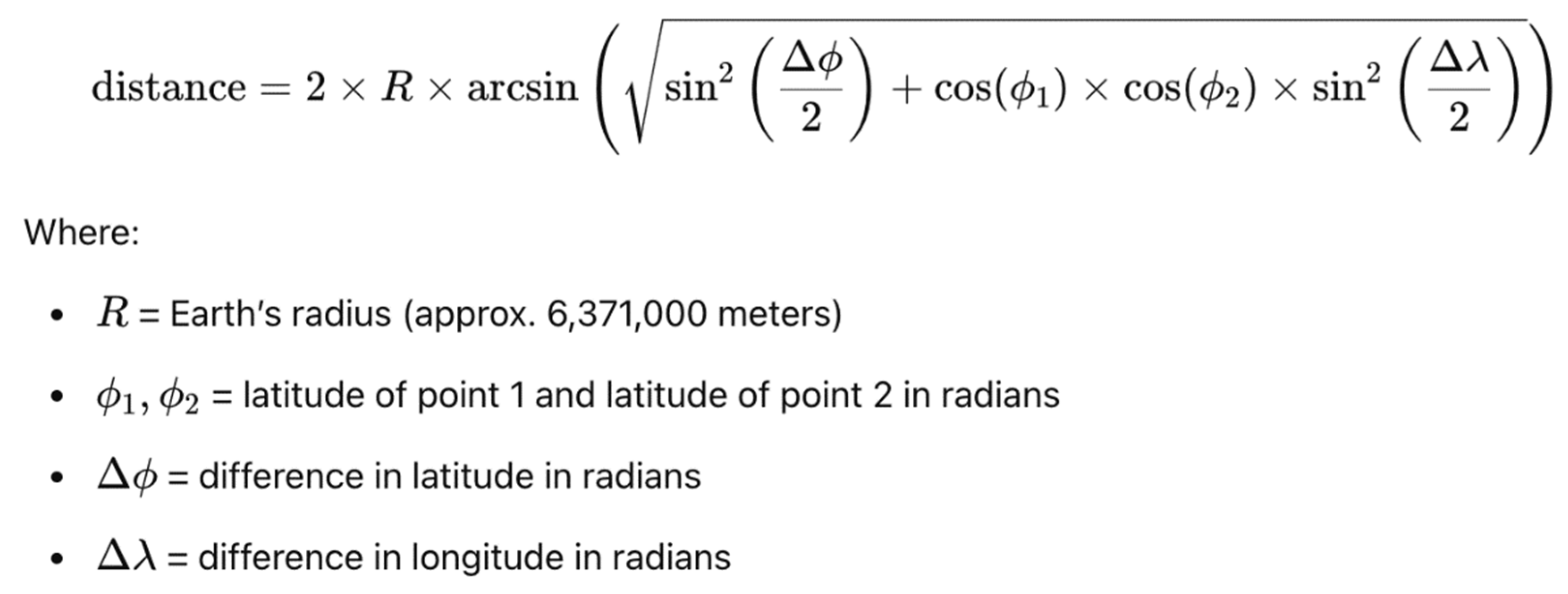
Figure 7.
Formula used for calculating the bearing between two GPS coordinates [screenshot].
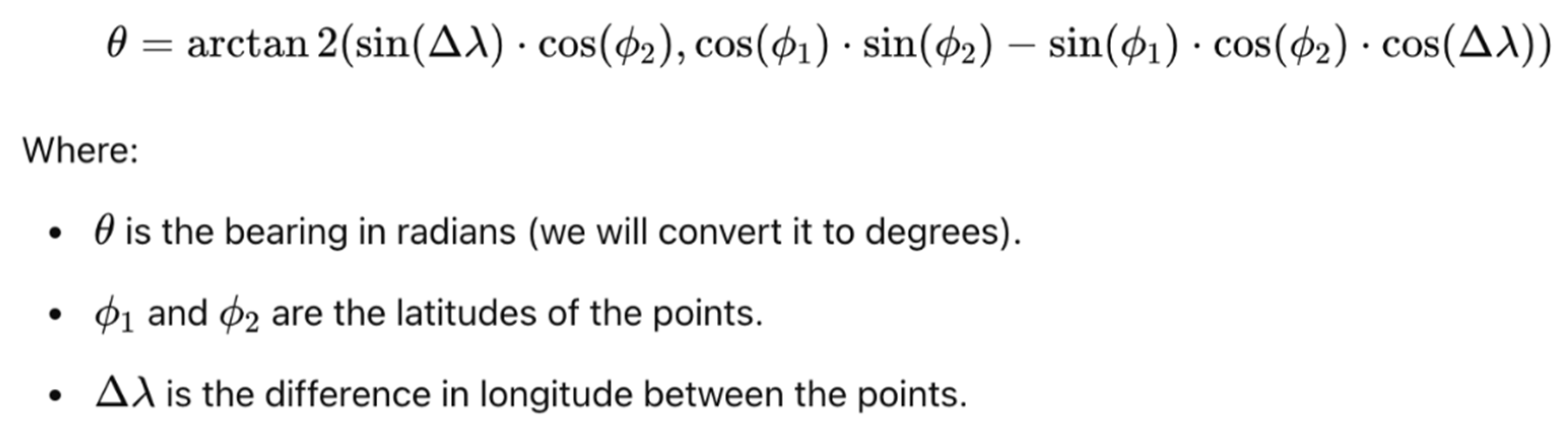
Figure 8.
Turning angle formula [screenshot]. .

Figure 9.
Figure 9. Speed overtime visualization [image].
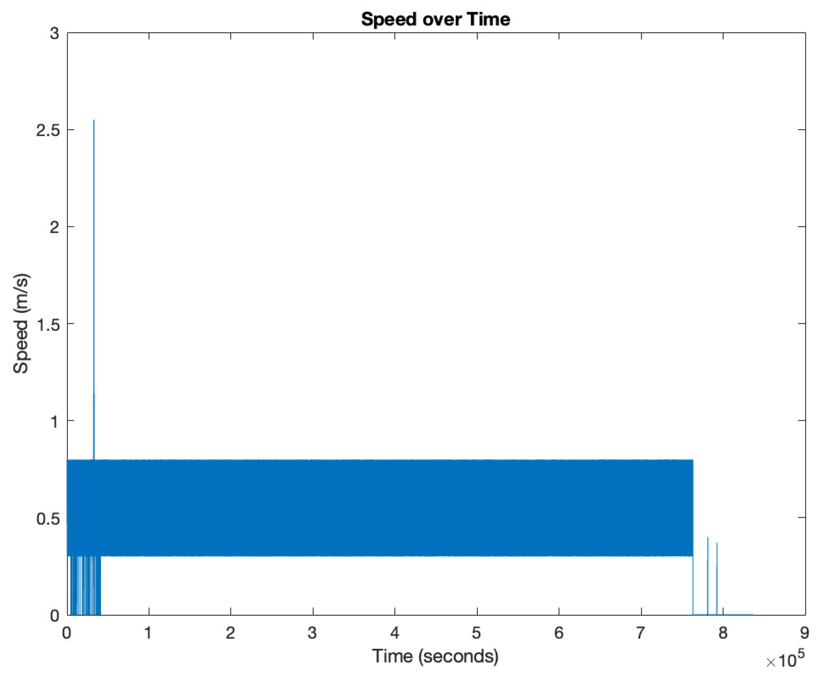
Figure 10.
Turning Angle Distribution Visualization [image]. .
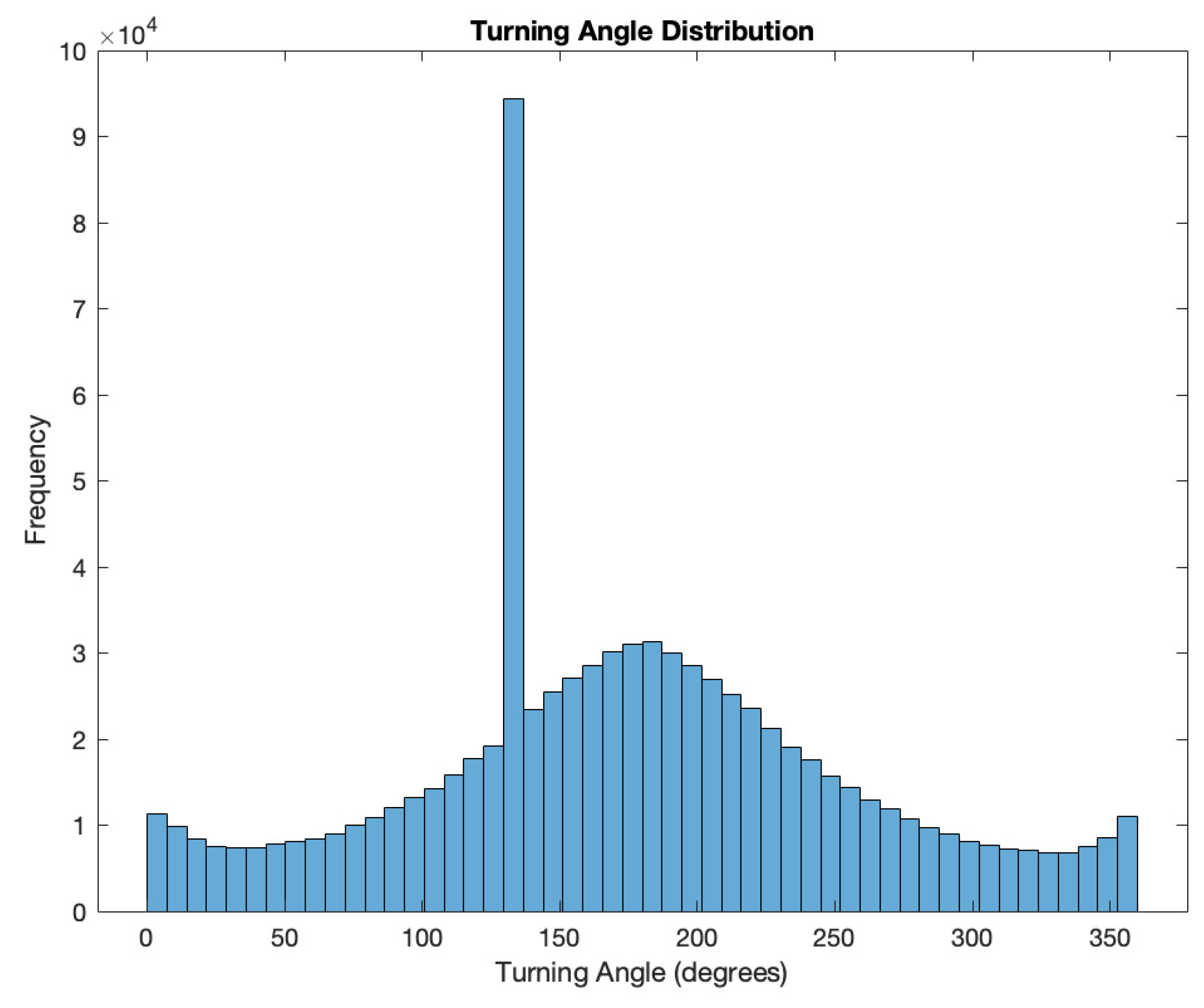
Figure 11.
Resting vs Moving State Visualization [image]. .
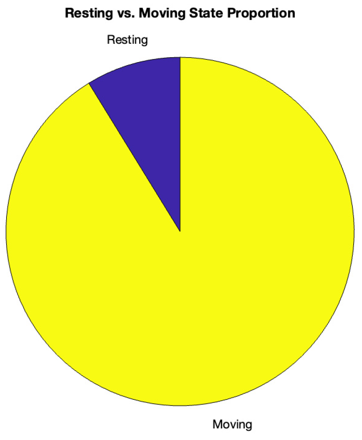
Figure 12.
Speed over time with trend visualization [image].
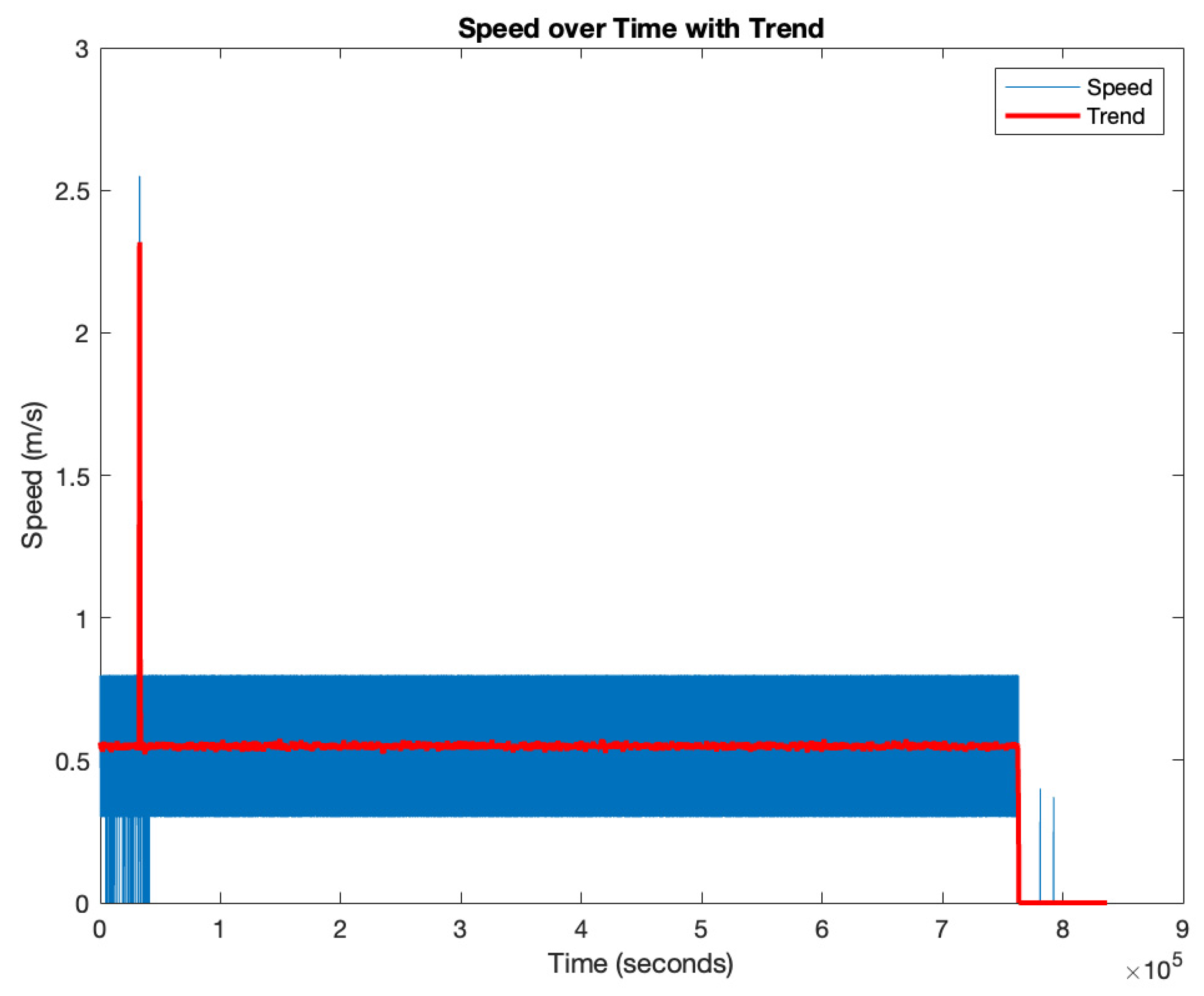
Figure 13.
Pathway of tracker from launch point until end point [image].
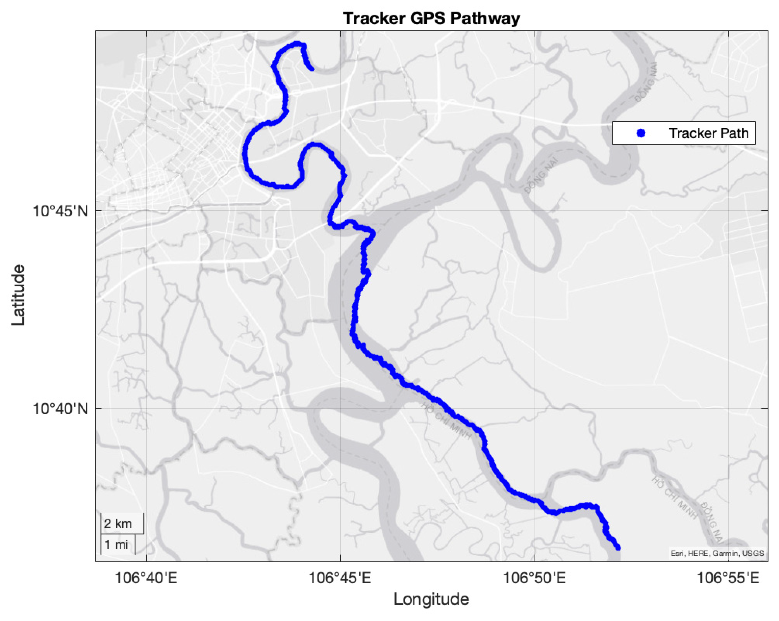
Figure 14.
State Transition Diagram [image].
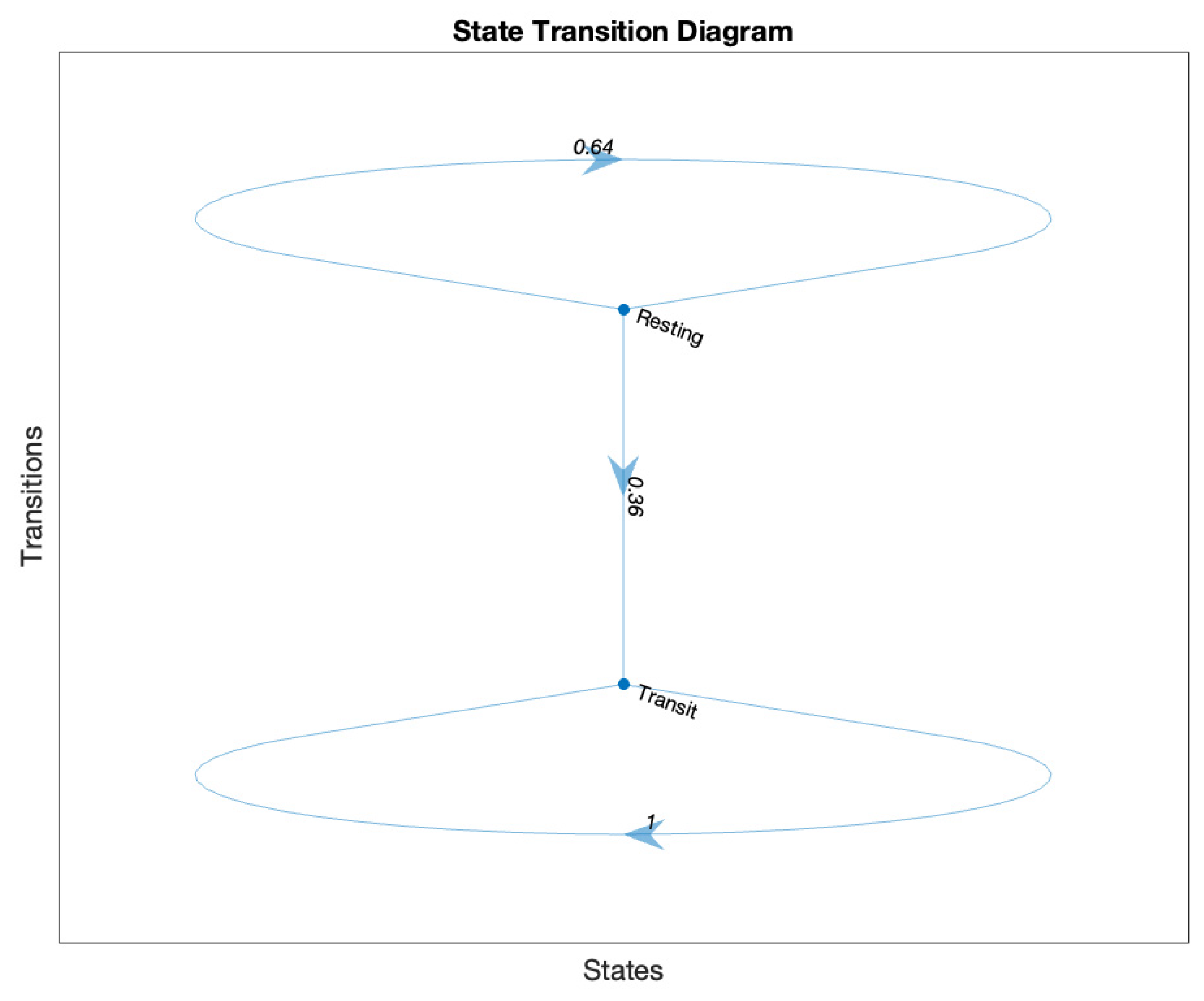
Figure 15.
Speed, Gyroscopic, and Accelerometer Data during Speed Spike Event .
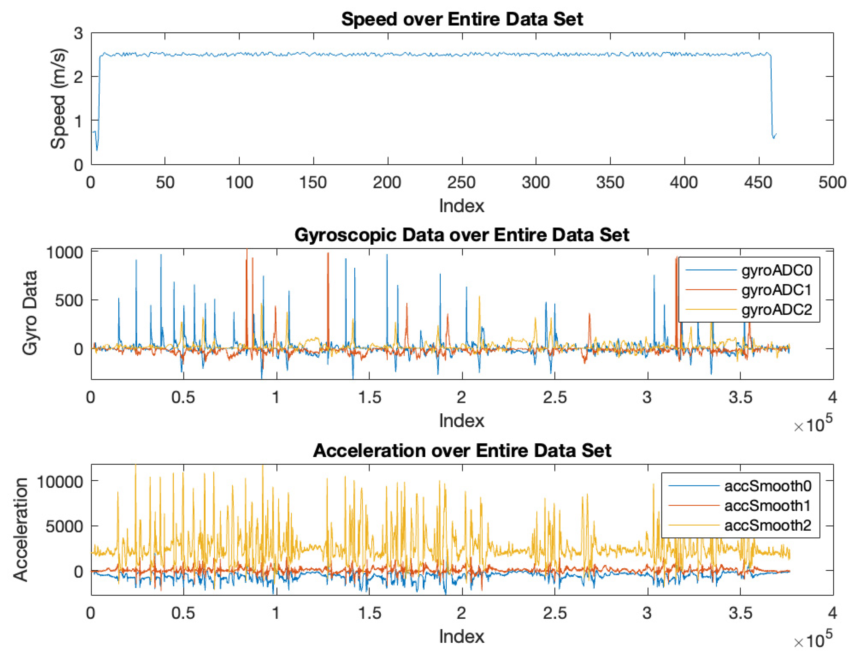
Figure 16.
Overview of Speed Spike Event Location.
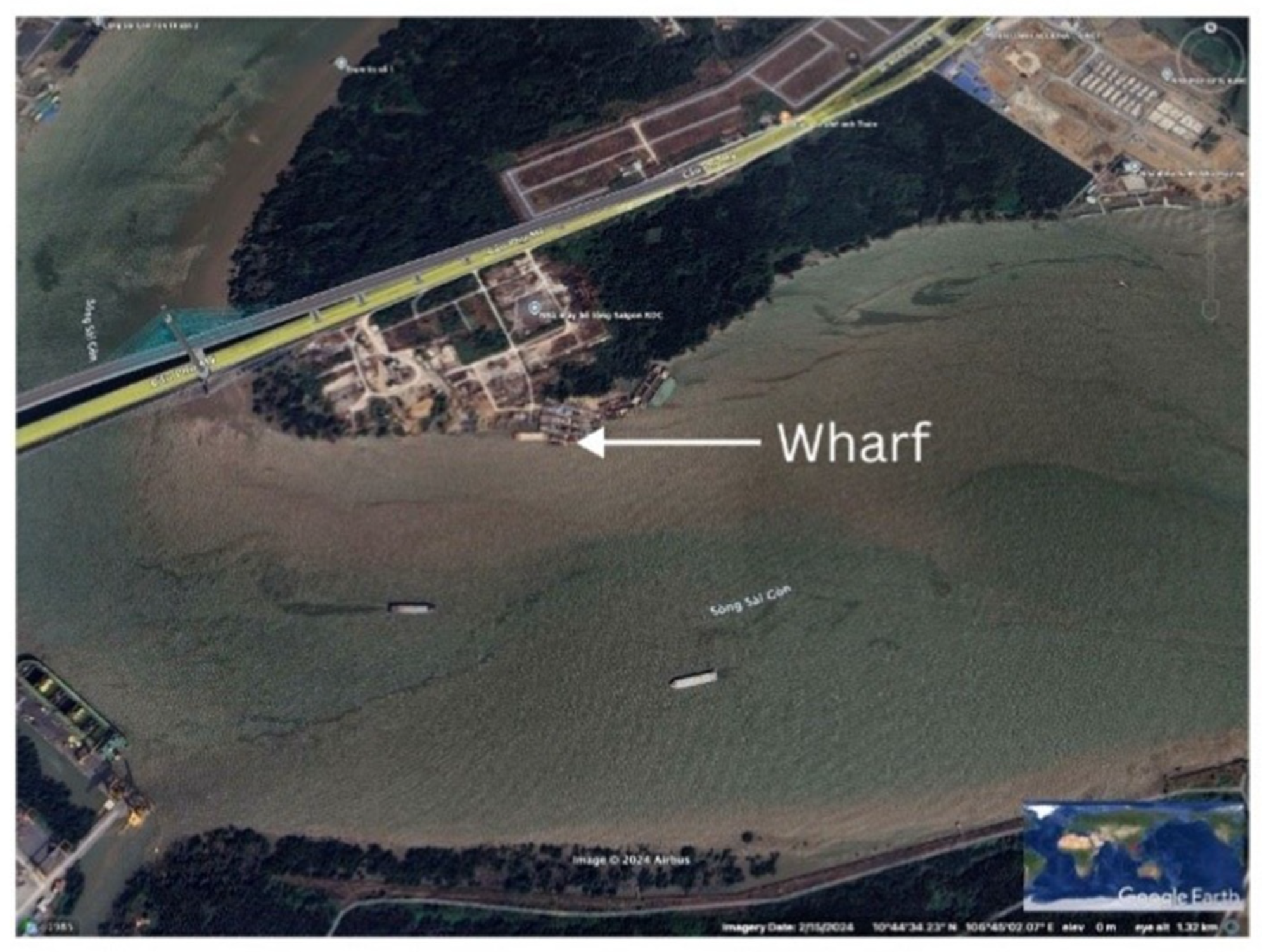
Figure 17.
Detailed View of GPS Track During Speed Spike.
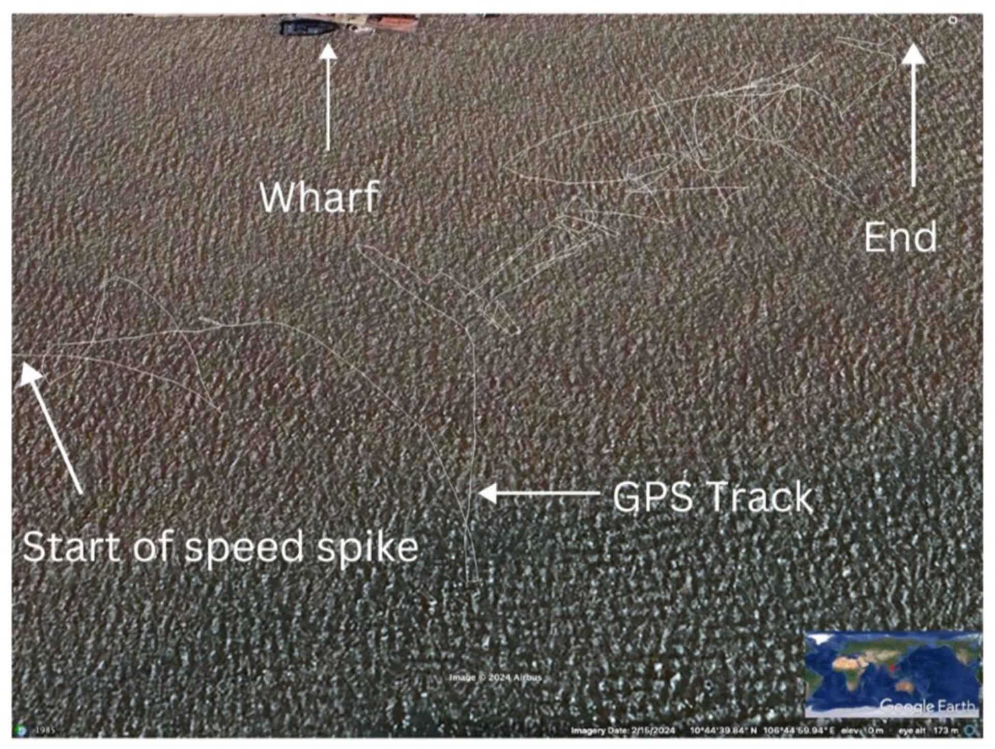

Table 1.
Initial data summary [table].
| Metric | Mean | Standard Deviation |
Units | Description |
|---|---|---|---|---|
| Speed | 0.5 | 0.21 | m/s | Average speed of the tracker with variability in movement speed. |
| Acceleration | 0 | 0.19 | m/s² | Average change in speed, indicating steady movement overall. |
| Bearing/Heading | 187.66 | N/A | degrees | Average directional heading, suggesting movement towards the SSW. |
| Distance Travelled | 205,744.51 | N/A | meters | This represents the total distance covered between the first and last recorded GPS points in the dataset. |
| Turning Angle | 174.77 | N/A | degrees | Average turning angle, indicating frequent near-complete direction changes. |
Table 2.
Estimated Transition and Emission Matrices [table]. .
| Matrix | State Transition/Emission | Probability |
|---|---|---|
| Estimated Transition Matrix | Resting → Resting (State 1 to State 1) | 0.644 |
| Resting → Transit (State 1 to State 2) | 0.356 | |
| Transit → Transit (State 2 to State 2) | 1 | |
| Estimated Emission Matrix | Low Speed while in Resting | 0.1275 |
| Medium Speed while in Resting | 0.7934 | |
| High Speed while in Resting | 0.0792 | |
| Low Speed while in Transit | 0.0165 | |
| Medium Speed while in Transit | 0.6152 | |
| High Speed while in Transit | 0.3684 |
Disclaimer/Publisher’s Note: The statements, opinions and data contained in all publications are solely those of the individual author(s) and contributor(s) and not of MDPI and/or the editor(s). MDPI and/or the editor(s) disclaim responsibility for any injury to people or property resulting from any ideas, methods, instructions or products referred to in the content. |
© 2024 by the authors. Licensee MDPI, Basel, Switzerland. This article is an open access article distributed under the terms and conditions of the Creative Commons Attribution (CC BY) license (http://creativecommons.org/licenses/by/4.0/).
Copyright: This open access article is published under a Creative Commons CC BY 4.0 license, which permit the free download, distribution, and reuse, provided that the author and preprint are cited in any reuse.


