
Submitted:
11 November 2024
Posted:
12 November 2024
You are already at the latest version
Abstract
Coded aperture imaging (CAI) is a well-established computational imaging technique consisting of two steps namely optical recording of an object using a coded mask followed by a computational reconstruction using a computational algorithm using a pre-recorded point spread function (PSF). In this tutorial, we introduce a simple yet elegant technique called Spatial Ensemble Mapping (SEM) for CAI that allows us to tune axial resolution post-recording from a single camera shot recorded using an image sensor. The theory, simulation studies, and proof-of-concept experimental studies of SEM-CAI are presented. We believe that the developed approach will benefit microscopy, holography, and smartphone cameras.
Keywords:
Coded aperture imaging
; incoherent imaging
; coded aperture
; diffractive optics
; holography
; interferenceless coded aperture correlation holography
1. Introduction
Computational imaging (CI) is a rapidly evolving field of research with incredible capabilities [1]. Coded aperture imaging is one of the oldest sub-fields of CI developed to overcome the challenges associated with manufacturing lenses for non-visible regions of the electromagnetic spectrum such as X-rays and Gamma rays [2,3,4]. In CAI, the light from an object is modulated by a coded mask (CM) and the response to object intensity (IROI) is recorded by an image sensor. Like any imaging system, CAI involves a calibration step where the point spread function (IPSF) is recorded using the CM. The image of the object is reconstructed by processing IPSF with IROI using a computational reconstruction algorithm. While without a doubt CAI enabled imaging for extreme wavelengths without a lens, the quality of images obtained from CAI after the above-described multiple steps did not reach the level of that obtained from a lens. Therefore, CAI evolved over the years with developments in two directions namely towards an advanced CM and computational algorithm. Some notable inventions along the direction of CM are the developments of the Fresnel zone aperture [5], uniformly redundant array mask [6], modified uniformly redundant array mask [7], and scattering mask [8]. Similarly, many developments in computational reconstruction methods such as phase-only filter [9], Weiner deconvolution (WD) [10], and Lucy-Richardson algorithm were developed [11,12].
In 2017, interferenceless coded aperture correlation holography (I-COACH) was developed which extended CAI to 3D imaging along three spatial dimensions [13]. It must be noted that CAI along 3D (2D space and spectrum) was achieved much earlier [14]. When I-COACH was developed using a quasi-random phase mask, it was found that the existing computational reconstruction methods did not support an image reconstruction with a high signal-to-noise ratio (SNR). This led to the development of numerous computational reconstruction methods such as non-linear reconstruction (NLR) [15], Lucy-Richardson-Rosen algorithm (LRRA) [16], and incoherent non-linear deconvolution with an iterative algorithm (INDIA) [17].
The development of I-COACH had a significant impact on the field of imaging and holography [2]. I-COACH was able to achieve imaging capabilities that were believed to be impossible in imaging technology. Some key developments include, the development of a 4D imaging capability along 3D space and spectrum using a monochrome camera [18], extending the field-of-view beyond the limits of the image sensor [19], synthetic aperture imaging system which requires scanning only along the periphery with a scanning ratio < 0.01 (scanning ratio = Scanned area/total area) [20] and imaging resolution enhancement [21,22]. Recently, a new problem ‘tuning axial resolution independent of lateral resolution’ has been addressed extensively using I-COACH techniques [23,24,25,26]. In 2024, the above problem has been solved creatively with capabilities to tune axial and spectral resolutions post-recording [27,28]. However, the above methods require multiple camera shots.
In this tutorial, we introduce a simple yet valuable technique called spatial ensemble mapping (SEM) where an ensemble of diverse diffraction patterns is mapped to different radii of the area of the image sensor. Therefore, different areas of the image sensor have different axial correlation lengths affecting the respective resolutions along the longitudinal space. But the lateral resolution remains the same as the numerical aperture (NA) which controls the lateral correlation lengths remains the same yielding lateral resolution independent of the area selection in the image sensor. Therefore, the developed approach allows tuning the axial resolution post-recording from a single camera recording without affecting the lateral resolution. Besides, this approach creates a new interdependency between the field of the image sensor to the axial resolution which does not exist in conventional imaging as well as CAI. Both direct as well as inverse relations between the area of the sensor and axial resolution can be obtained. While we demonstrate the SEM concept for only axial resolution, the developed method can be used to tune other imaging characteristics such as spectral resolution, lateral resolution, and 3D image location.
The manuscript consists of six sections. The methodology is presented in the next section. In the third section, presents the simulation studies. The experimental studies are presented in the fourth section. The results are discussed in the fifth section. The conclusion and future perspectives of the study are presented in the final section of the manuscript.
2. Materials and Methods
The proposed SEM-CAI consists of two components namely CM design and imaging process as shown in Figure 1. In the CM design, the SEM concept is applied where the phase functions of several diffractive elements with different axial propagation characteristics are mapped to different regions of the image sensor mutually exclusively – without spatial overlap. This is achieved by combining unique linear phases (LPs) with the phase functions of different diffractive elements. There are no rules on what diffractive elements are to be used, where to map the functions on the image sensor, and what relationship between the area of the image sensor and axial resolution is needed. All the above can be selected depending upon the requirements ‘on-demand’.
—refers to complex conjugate following a Fourier transform; - Inverse Fourier transform; Rn is the nth solution and n is an integer, when n = 1, IRn = IROI; NLR – Non-linear reconstruction; ML – Maximum Likelihood; α and β are varied from -1 to 1.
In this study, three diffractive elements namely a diffractive axicon and two Fresnel zone plates (FZPs) with different focal distances are selected. The diffraction pattern generated by the axicon is mapped to the origin of the image sensor. The diffraction patterns from the FZPs are mapped at certain distances away from the center in the positive and negative sides along the horizontal direction. The above mapping was designed such that when the area of the recording is increased, the axial resolution is increased. When the area includes only the diffraction pattern of axicon, a low axial resolution is obtained. When the area includes the diffraction patterns of axicon and FZP1 then the axial resolution increases and when the area includes all the diffraction patterns, then the axial resolution is increased further. It is possible to have greyscale masks that can increase the contribution of one of the diffraction patterns with respect to the other. The maximum axial resolution is given by the NA, ~λ/NA2. The proposed SEM-CAI allows to tune the axial resolution from a certain value to the maxima but cannot be used to achieve super axial resolution.
In this study, only spatially incoherent and temporally coherent light sources are considered. The phase functions of the diffractive axicon, FZP1 and FZP2 are given as , and respectively, where Λ is the period of the axicon, , f1 and f2 are the focal distances of FZP1 and FZP2 respectively. The three LPs assigned to the above three masks are , where k = 1, 2 and 3. The above LPs are combined with the phase functions of diffractive elements as resulting in a complex function. A recently developed computational algorithm named transport of amplitude into phase based on Gerchberg-Saxton algorithm (TAP-GSA) is used to convert the complex function ΨCM into a phase only function as shown in Figure 1a [29]. Therefore, the CM can be expressed as . The resulting phase-only CM is used for the next step – imaging process. The above approximation is achieved by applying amplitude and phase constraints in the sensor plane. The generated amplitude matrix during forward propagation is replaced by the amplitude matrix obtained for the forward propagation of the complex CM. The phase matrix is replaced as above but partially quantified by a term called degrees of freedom given by the number of pixels replaced in the matrix to the total number of pixels of the phase matrix. After several iterations, a phase-only equivalent of a complex CM is obtained. The application of TAP-GSA is crucial to the implementation of SEM as the alternative random multiplexing method developed for Fresnel incoherent correlation holography (FINCH) results in speckle noises affecting the overall tunability of axial resolution [30,31]. When TAP-GSA was implemented to FINCH, instead of the random multiplexing, a significant improvement in SNR and light throughput was observed. The commented MATLAB code for implementing TAP-GSA is provided in the supplementary materials (Supplementary_code1.txt) [32].
The imaging process shown in Figure 1b in the next step can be mathematically expressed as follows: A point object is considered in the object domain from the CM. The complex amplitude reaching the CM is given as , where is the amplitude, Q is a quadratic phase function given as , L is the linear phase function given as and C1 is a complex constant. The complex amplitude after the CM is given as which is propagated by a distance of zh and recorded by an image sensor whose intensity distribution is given as
where ‘’ is a 2D convolutional operator and is the location vector in the sensor plane. However, unlike the previous developments of CAI and I-COACH, there is a new equality in the proposed approach which is
where C11, C12, C13 are complex constants. The above equality is possible because of SEM which has a much deeper meaning. In Eq. (1), there is self-interference between the ensemble of optical fields, whereas the equality shown in Eq. (2), has a unique behavior , where A represents the ensemble of diffracted fields generated by the CM. In the first case, where there is self-interference, the nature of light is spatially incoherent and temporally coherent which matches with the source specifications. In the second case due to SEM, the fields generated by the CM that are mapped to different locations behave as if they are not coherent with respect to one another even though derived from the same object point. This is a fundamental change through SEM which allows such tunability. Equation (1) can be expressed as
where , and are PSFs of axicon, FZP1 and FZP2 respectively. By selecting the area of the recordings, it is possible to control the contributions from the different diffractive elements. has a low sensitivity to changes in depth and wavelength, whereas and have a high sensitivity to changes in depth and wavelength as given by the numerical aperture NA. Therefore, when there is a change in depth and only the central region of the recording containing only the diffracted field of axicon is considered, then the correlation curve given as will be broad as , where ‘ is a 2D correlation operator. The same argument also applies to changes in wavelength. Let us consider the other cases when the area includes a diffracted field of FZP in addition to that from axicon, will be sharper than the previous case as . Once again, the above is true for the wavelength. In this way, the axial resolution can be tuned between the limits of axicon and lens which are and respectively, where D is the diameter of the CM [33,34,35,36,37].
The proposed SEM-CAI is a linear, shift-invariant system and therefore,
A 2D object with N points can be represented mathematically as a collection of N Delta functions given by
where aj’s are constants. The response to object intensity based on the assumption that a spatially incoherent and temporally coherent light source is considered is given as
There are numerous deconvolution methods that can be applied and, in this study, LRRA and WD are used for reconstructing the object information as shown in Figure 1b. The (n+1)th reconstructed image is given as
where ‘’ indicates the NLR operation which is given as , where is the Fourier transform of X and A and B are the two matrices. The α and β are tuned between -1 and 1 to obtain the optimal entropy and a fast convergence. The LRRA has been thoroughly discussed in [16,17]. The algorithm is briefly summarized here. The LRRA begins with an initial guess solution of the object which is the IROI. In principle, the initial guess can be any matrix, even random, but to improve the convergence, the initial guess is selected as IROI. This initial guess is convolved with IPSF to obtain IROI’ which will be IROI if the initial guess was the actual solution. The ratio between the recorded response to object intensity and obtained matrix given as Ratio = IROI/IROI’ is calculated. Then the Ratio is processed with IPSF using NLR to obtain the Residue. The Residue is multiplied to the previous solution which is the initial guess solution to obtain the next solution (n=2). This process is iterated until an optimal solution is obtained. During the reconstruction, the values of α and β are set to a value and are not changed once the iteration is started. The commented MATLAB code is provided in the supplementary materials (Supplementary_code2.txt).
3. Simulation Results
The simulation studies were carried out in MATLAB software (version R2022a). A matrix size of 500 × 500 pixels, a pixel size Δ = 10 μm, wavelength λ = 632.8 nm, object distance zs = 1 m, and a recording distance (distance between CM and image sensor) zh = 0.2 m are selected. Three greyscale diffractive elements were designed: Axicon with Λ = 80 μm with no linear phase (ak = bk = 0), FZP1 (f1 = 0.16 m) (ak = -0.007, bk = 0) and FZP2 (f2 = 0.17 m) (ak = 0.01, bk = 0). The phase images of the masks are shown in Figure 2a–c respectively. The magnitude and phase of the complex function of CM obtained by the sum of the three phase-only functions of a diffractive axicon, FZP1 with LP2 and FZP2 with LP3 are shown in Figures 2d and 2e respectively. The phase-only CMs obtained by random multiplexing and TAP-GSA with a degree of freedom of 0.16 are shown in Figure 2f and 2g respectively. The diffraction pattern obtained at a distance of 0.2 m from the CM for Figure 2d,e, Figure 2f,g are shown in Figure 2h, 2i and 2j respectively. The magnified regions of the intensity matrices for the above three cases show a reduced scattering noise with TAP-GSA.
The axial behavior is simulated next. The IPSF is simulated for different values of zs and processed with IPSF corresponding to a single value of zs as , where zs = 1 m and Δzs is tuned from -0.5 m to 0.5 m. The normalized curves of for five cases of masks applied to recordings are shown in Figure 3. It can be seen that by selecting an appropriate mask, different strengths of axial correlation lengths can be contributed from different areas of the recordings resulting in a desired effective axial resolution.
The simulated optical experiments are discussed next. Two ‘Smiley’ objects were selected for the study as shown in Figure 4a and 4b respectively. The two objects were separated by a distance of 20 cm. Even though there are clear variations in the curves shown in Figure 3 for different cases of the masks, in imaging it is challenging to observe minor changes in axial resolution. Therefore, for the simulation study, only three cases are considered corresponding to Masks – Mask1, Mask2, and Mask4. The images of the simulated IPSFs, IROIs, and IRs for Mask1, Mask2, and Mask4 are shown in Figure 4. From the results, it can be seen that the axial resolution increases from Mask1 to Mask4. The reconstructed second smiley object – Test object 2 becomes more and more blurred with an increase in the axial resolution. For all the above cases, LRRA was applied with three to five iterations with α = 0, β = 0 to 0.2.
4. Experiments
The schematic and a photograph of the experimental setup are shown in Figure 5a,b. The experimental setup includes the following optical components: Light emitting diode (LED) from Thorlabs with 940 mW power, operating at a wavelength of λ = 660 nm and has a bandwidth of Δλ = 20 nm; two irises; polarizer; three refractive lenses (RLs) with a focal length f = 3.5 cm, f = 5 cm and f = 5 cm; pinhole of size 50 μm; beam splitter (BS); Exulus-4K 1/M spatial light modulator (SLM) from Thorlabs with 3840 × 2160 pixels and a pixel size of 3.74 μm and Zelux CS165MU/M monochrome image sensor with 1440 × 1080 pixels with a pixel size of ~3.5 µm.
The light from the LED is controlled by an iris and collimated by an RL (f = 3.5 cm). The collimated beam is passed through a polarizer, which is oriented along the active axis of the SLM. Two objects were created by shifting a pinhole of 50 μm in horizontal and vertical directions. Object 1 (Two points along horizontal direction separated by 120 μm) and Object 2 (Two points along vertical direction separated by 120 μm) are created. The object is critically illuminated by an RL (f = 5 cm). The light beam from the object is collimated by an RL (f = 5 cm) and the beam size is controlled by another iris. The collimated light beam enters the BS and is incident on the SLM. The CM was created by combining two FZPs (with a focal length of 16 cm) and one diffractive axicon (with Λ = 187 μm) using TAP-GSA with a degree of freedom of 75%. The phase-only CM from TAP-GSA is displayed on the SLM which modulates the light beam creating the diffraction spots of the two FZPs and diffractive axicon at predefined locations on the image sensor. The IPSF and IROI were recorded by the image sensor located at a distance of 20 cm from the SLM. The IPSF was recorded using a 50 μm pinhole. Object 1 and Object 2 were recorded at two different depths zs = 5 cm and zs = 5.4 cm respectively. The object information was reconstructed by processing IPSF and IROI using LRRA. The experimental results are shown in Figure 6. The experimentally recorded IPSF and IROI are shown in Figure 6a,b respectively. Two masks Mask1 and Mask2 were applied to the recorded IPSF and IROI and reconstructed. The images of the masks - Mask1 and Mask2 and reconstructed images are shown in Figure 6c, 6e, 6d and 6f respectively. The phase image of the CM generated using TAP-GSA with degrees of freedom of 75% is shown in Figure 6g. Comparing the reconstruction results of Figure 6d,f, the axial resolution of 6f is better than that of 6d demonstrating the tunability of axial resolution post-recording. In the case of Mask1 (Figure 6c), there is contribution only from the diffractive axicon which has a long axial correlation length resulting in a low axial resolution. In the case of Mask2 (Figure 6e), there is contribution from two FZPs and a diffractive axicon resulting in short axial correlation length. The shorter correlation length for Mask2 arises due to the averaging effect of correlation lengths corresponding to diffractive axicon and FZPs. However, in the above two cases, the lateral correlation length is the same as the NA is constant for both cases. In all the above cases, the typical range of α, β and the number of iterations for LRRA are 0 to 0.4, 1 and 10 to 30 respectively. The experimental results are matched with the simulation results and validate the theory of SEM-CAI.
5. Discussion
In this study, a simple yet useful technique called SEM has been introduced in CAI for tuning axial resolution independent of lateral resolution post-recording. Like any new technique, an advancement is made here with SEM-CAI with a compromise on the field of view. The above approach is suitable only for recording events and scenes with a limited field of view. The above understanding also gives rise to a question. Can direct imaging approaches be applied here by reducing the field of view and tiling different configurations along the x and y directions on the image sensor? This is impossible due to the interdependency between lateral and axial resolutions in direct imaging approaches. Even if that condition is relaxed, the direct imaging approach can allow only discrete tuning of axial resolution along the tiled images. The interdependency between lateral and axial resolutions by NA will cause a change in lateral resolution also along the tiled images.
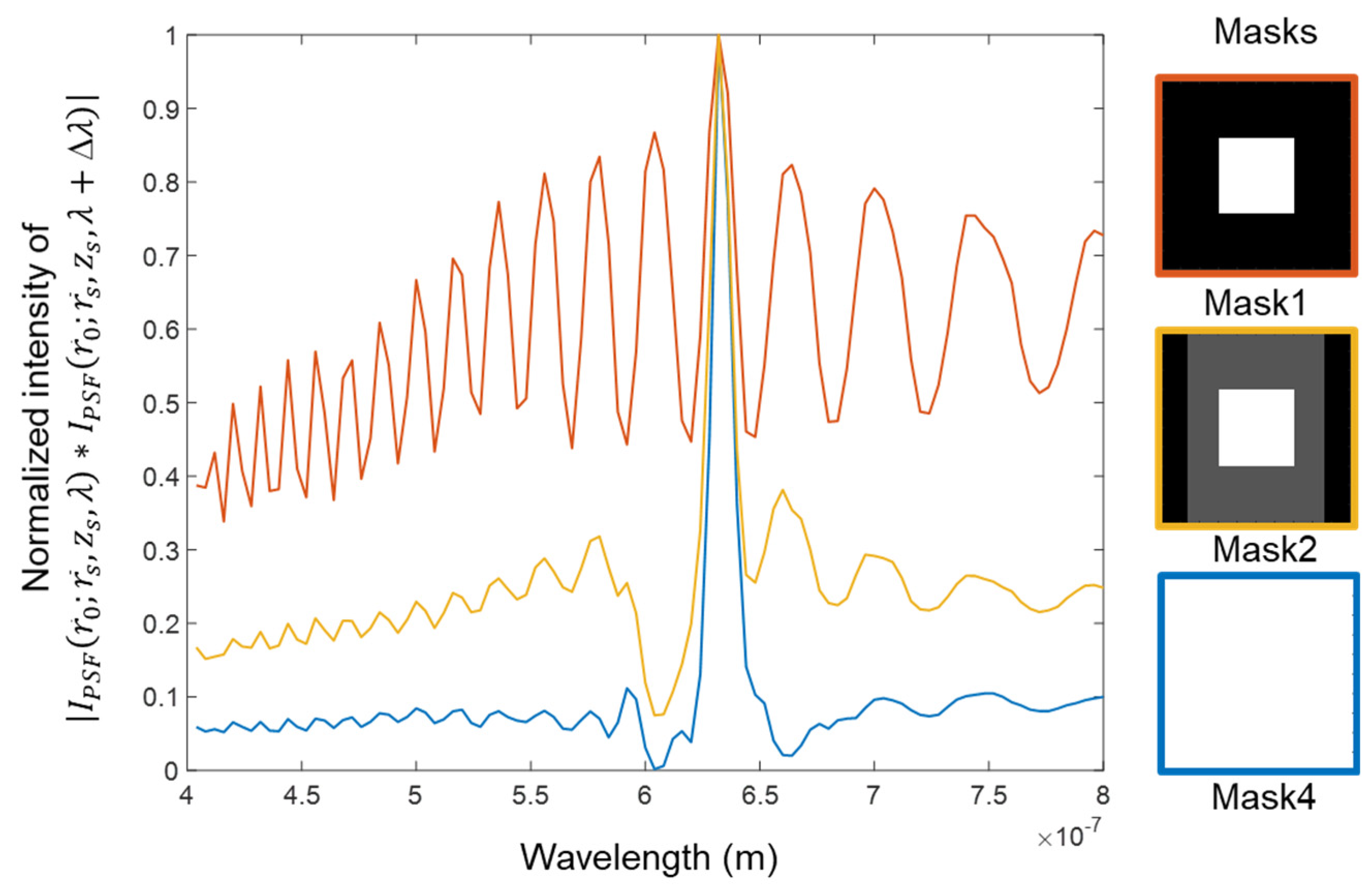
The developed SEM-CAI, even though has been demonstrated only for tuning axial resolution independent of lateral resolution, the concept can be extended to tuning spectral resolution independent of lateral resolution as well. The simulation results for tuning spectral resolution post-recording using a monochrome sensor for three masks Mask1, Mask2 and Mask4 were carried out. The spectral correlation curves obtained from for a wavelength variation between 400 to 800 nm for the three masks are shown in Figure 7. As it is seen, the spectral resolution improves from Mask1 to Mask4. The same approach can also be used to tune lateral resolution which has not been discussed in [27,28] and so far, not possible after recording a picture or a video. However, a low lateral resolution does not have any useful application.
This tutorial unifies also the previous studies on this topic using a hybrid imaging system with a lens and an axicon and an Airy beam generator [27,28]. In this study, only two types of elements namely a diffractive lens and a diffractive axicon have been used. However, it is possible to use a wide range of diffractive elements and beams such as self-rotating beams [25,38,39], Airy beams [40,41], and Higher order Bessel beams [42,43,44]. In this study, only three beams have been used, however lesser or a greater number of beams can be used to achieve axial and spectral tunability post-recording.
6. Conclusions
Spatial ensemble mapping (SEM) has been introduced to the CAI technique. In SEM, different beams are mapped to different lateral locations in the image sensor. By this simple, yet fundamental change, the imaging properties can be made flexible. The goal of SEM is to have different strengths of one or more imaging characteristics available as components of a parameter and one or more components can be combined depending upon the requirements to obtain ‘on-demand imaging’ characteristics. In this study, three diffractive elements namely two diffractive lenses and one diffractive axicon were combined using TAP-GSA to obtain a single phase-only diffractive element with minimal scattering. The diffraction patterns from the above three elements were positioned at different locations. A diffractive axicon has a long axial correlation length whereas a diffractive lens has a short axial correlation length. Therefore, by combining the diffraction patterns with different strengths, a desired correlation length can be engineered. In this study, only LRRA and WD have been used but any reconstruction algorithm such as NLR, or INDIA can be used. This technique can be expanded and investigated for a wide range of optical beams such as self-rotating beams [25], Airy beams [45], etc., tuning different parameters such as spectral resolution [46], lateral resolution [47,48] and 3D image steering [49,50]. One of the challenges that exists with CAI that precludes its application to commercial imaging systems is the lack of a robust computational reconstruction method that can reconstruct images with a high SNR. We believe that the developed SEM-CAI with the development of advanced computational reconstruction methods will benefit existing CAI techniques, I-COACH-based techniques, microscopy, and smartphone cameras. While the developed technique has been demonstrated only with spatially incoherent light and for intensity imaging, they can be extended for coded aperture based phase imaging applications [51,52,53,54].
Author Contributions
Conceptualization, V.A.; methodology, S.G., A.P.I.X., N. J., V. T. and V.A.; validation, V.A., V. T., N. J., A.P.I.X. and S.G.; resources, V.A.; writing—original draft preparation, all the authors; supervision, V. A.; funding acquisition, V. A. All authors have read and agreed to the published version of the manuscript.
Funding
This research was funded by European Union’s Horizon 2020 research and innovation programme grant agreement No. 857627 (CIPHR).
Institutional Review Board Statement
Not applicable.
Informed Consent Statement
Not applicable.
Data Availability Statement
Data can be obtained from the corresponding author upon reasonable request.
Conflicts of Interest
The authors declare no conflicts of interest.
References
- Mait, J.N.; Euliss, G.W.; Athale, R.A. Computational imaging. Adv. Opt. Photon 2018, 10, 409–483. [Google Scholar] [CrossRef]
- Rosen, J.; Vijayakumar, A.; Kumar, M.; Rai, M.R.; Kelner, R.; Kashter, Y.; Bulbul, A.; Mukherjee, S. Recent advances in selfinterference incoherent digital holography. Adv. Opt. Photonics 2019, 11, 1–66. [Google Scholar] [CrossRef]
- Ables, J.G. Fourier transform photography: A new method for X-ray astronomy. Proc. Astron. Soc. 1968, 1, 172. [Google Scholar] [CrossRef]
- Dicke, R.H. Scatter-hole cameras for X-rays and gamma rays. Astrophys. J. 1968, 153, L101. [Google Scholar] [CrossRef]
- Mertz, L. & Young, N. O. Fresnel transformation of images. In Proc. ICO Conference on Optical instruments and Techniques (ed. K. J. Habell) 305–310 (Chapman and Hall, London, 1962).
- Fenimore, E.E.; Cannon, T.M. Coded aperture imaging with uniformly redundant arrays. Appl. Opt. 1978, 17, 337–347. [Google Scholar] [CrossRef]
- Olmos, P.; Cid, C.; Bru, A.; Oller, J.C.; de Pablos, J.L.; Perez, J.M. Design of a modified uniform redundant-array mask for portable gamma cameras. Appl. Opt. 1992, 31, 4742–4750. [Google Scholar] [CrossRef]
- Singh, A.K.; Pedrini, G.; Takeda, M.; Osten, W. Scatter-plate microscope for lensless microscopy with diffraction limited resolution. Sci. Rep. 2017, 7, 10687. [Google Scholar] [CrossRef]
- Horner, J.L.; Gianino, P.D. Phase-only matched filtering. Appl. Opt. 1984, 23, 812–816. [Google Scholar] [CrossRef]
- Woods, J.W.; Ekstrom, M.P.; Palmieri, T.M.; Twogood, R.E. Best linear decoding of random mask images. IEEE Trans. Nucl. Sci. 1975, 22, 379–383. [Google Scholar] [CrossRef]
- Richardson, W.H. Bayesian-Based Iterative Method of Image Restoration. J. Opt. Soc. Am. 1972, 62, 55–59. [Google Scholar] [CrossRef]
- Lucy, L.B. An iterative technique for the rectification of observed distributions. Astron. J. 1974, 79, 745. [Google Scholar] [CrossRef]
- Vijayakumar, A.; Rosen, J. Interferenceless coded aperture correlation holography–a new technique for recording incoherent digital holograms without two-wave interference. Opt. Express 2017, 25, 13883–13896. [Google Scholar] [CrossRef] [PubMed]
- Wagadarikar, A.; John, R.; Willett, R.; Brady, D. Single disperser design for coded aperture snapshot spectral imaging. Appl. Opt. 2008, 47, B44–B51. [Google Scholar] [CrossRef] [PubMed]
- Rai, M.R.; Vijayakumar, A.; Rosen, J. Non-linear adaptive three-dimensional imaging with interferenceless coded aperture correlation holography (I-COACH). Opt. Express 2018, 26, 18143–18154. [Google Scholar] [CrossRef]
- Anand, V.; Han, M.; Maksimovic, J.; Ng, S.H.; Katkus, T.; Klein, A.; Bambery, K.; Tobin, M.J.; Vongsvivut, J.; Juodkazis, S. Single-shot mid-infrared incoherent holography using Lucy-Richardson-Rosen algorithm. Opto-Electron. Sci. 2022, 1, 210006. [Google Scholar]
- Rosen, J.; Anand, V. Incoherent nonlinear deconvolution using an iterative algorithm for recovering limited-support images from blurred digital photographs. Opt. Express 2024, 32, 1034–1046. [Google Scholar] [CrossRef]
- Anand, V.; Ng, S.H.; Maksimovic, J.; Linklater, D.; Katkus, T.; Ivanova, E.P.; Juodkazis, S. Single shot multispectral multidimensional imaging using chaotic waves. Sci. Rep. 2020, 10, 13902. [Google Scholar] [CrossRef]
- Rai, M.R.; Vijayakumar, A.; Rosen, J. Extending the field of view by a scattering window in I-COACH system. Opt. Lett. 2018, 43, 1043–1046. [Google Scholar] [CrossRef]
- Bulbul, A.; Vijayakumar, A.; Rosen, J. Superresolution far-field imaging by coded phase reflectors distributed only along the boundary of synthetic apertures. Optica 2018, 5, 1607–1616. [Google Scholar] [CrossRef]
- Rai, M.R.; Vijayakumar, A.; Ogura, Y.; Rosen, J. Resolution Enhancement in Nonlinear Interferenceless COACH with a Point Response of Subdiffraction Limit Patterns. Opt. Express 2019, 27, 391–403. [Google Scholar] [CrossRef]
- Tamm, O.; Tiwari, V.; Gopinath, S.; Rajesway, A.S.J.F.; Singh, S.A.; Rosen, J.; Anand, V. Super-Resolution Correlating Optical Endoscopy. IEEE Access 2024, 12, 76955–76962. [Google Scholar] [CrossRef]
- Rai, M.R.; Rosen, J. Depth-of-field engineering in coded aperture imaging. Opt. Express 2021, 29, 1634–1648. [Google Scholar] [CrossRef] [PubMed]
- Anand, V. Tuning Axial Resolution Independent of Lateral Resolution in a Computational Imaging System Using Bessel Speckles. Micromachines 2022, 13, 1347. [Google Scholar] [CrossRef] [PubMed]
- Kumar, R.; Vijayakumar, A.; Rosen, J. 3D single shot lensless incoherent optical imaging using coded phase aperture system with point response of scattered airy beams. Sci. Rep. 2023, 13, 2996. [Google Scholar] [CrossRef]
- Bleahu, A.; Gopinath, S.; Kahro, T.; Angamuthu, P.P.; Rajeswary, A.S.J.F.; Prabhakar, S.; Kumar, R.; Salla, G.R.; Singh, R.P.; Kukli, K.; et al. 3D Incoherent Imaging Using an Ensemble of Sparse Self-Rotating Beams. Opt. Express 2023, 31, 26120–26134. [Google Scholar] [CrossRef]
- Gopinath, S.; Rajeswary, A.S.J.F.; Anand, V. Sculpting axial characteristics of incoherent imagers by hybridization methods. Opt. Lasers Eng. 2024, 172, 107837. [Google Scholar] [CrossRef]
- Gopinath, S.; Anand, V. Post-ensemble generation with Airy beams for spatial and spectral switching in incoherent imaging. Opt. Lett. 2024, 49, 3247–3250. [Google Scholar] [CrossRef]
- Gopinath, S.; Bleahu, A.; Kahro, T.; Rajeswary, A.S.J.F.; Kumar, R.; Kukli, K.; Tamm, A.; Rosen, J.; Anand, V. Enhanced design of multiplexed coded masks for Fresnel incoherent correlation holography. Sci. Rep. 2023, 13, 7390. [Google Scholar] [CrossRef]
- Rosen, J.; Brooker, G. Digital spatially incoherent Fresnel holography. Opt. Lett. 2007, 32, 912–914. [Google Scholar] [CrossRef]
- Katz, B.; Rosen, J.; Kelner, R.; Brooker, G. Enhanced resolution and throughput of Fresnel incoherent correlation holography (FINCH) using dual diffractive lenses on a spatial light modulator (SLM). Opt. Express 2012, 20, 9109–9121. [Google Scholar] [CrossRef]
- Rosen, J.; Alford, S.; Allan, B.; Anand, V.; Arnon, S.; Arockiaraj, F.G.; Art, J.; Bai, B.; Balasubramaniam, G.M.; Birnbaum, T.; Bisht, N.S. Roadmap on computational methods in optical imaging and holography. Appl. Phys. B 2024, 130, 166. [Google Scholar] [CrossRef] [PubMed]
- Golub, I. Fresnel axicon. Opt. Lett. 2006, 31, 1890–1892. [Google Scholar] [CrossRef]
- McLeod, J. The Axicon: A new type of optical element. J. Opt. Soc. Am. 1954, 44, 592–597. [Google Scholar] [CrossRef]
- Khonina, S.N.; Kazanskiy, N.L.; Khorin, P.A.; Butt, M.A. Modern Types of Axicons: New Functions and Applications. Sensors 2021, 21, 6690. [Google Scholar] [CrossRef]
- Khonina, S.N.; Porfirev, A.P. 3D transformations of light fields in the focal region implemented by diffractive axicons. Appl. Phys. B 2018, 124, 191. [Google Scholar] [CrossRef]
- Khonina, S.N.; Volotovsky, S.G. Application axicons in a large-aperture focusing system. Opt. Mem. Neural Netw. 2014, 23, 201–217. [Google Scholar] [CrossRef]
- Niu, K.; Zhao, S.; Liu, Y.; Tao, S.; Wang, F. Self-rotating beam in the free space propagation. Opt. Express 2022, 30, 5465–5472. [Google Scholar] [CrossRef]
- Niu, K.; Zhai, Y.; Wang, F. Self-healing property of the self-rotating beam. Opt. Express 2022, 30, 30293–30302. [Google Scholar] [CrossRef]
- Siviloglou, G.A.; Broky, J.; Dogariu, A.; Christodoulides, D.N. Observation of accelerating Airy beams. Phys. Rev. Lett. 2007, 99, 213901. [Google Scholar] [CrossRef]
- Vettenburg, T.; Dalgarno, H.I.C.; Nylk, J.; Coll-Lladó, C.; Ferrier, D.E.K.; Cizmar, T.; Gunn-Moore, F.J.; Dholakia, K. Light-sheet microscopy using an Airy beam. Nat. Methods 2014, 11, 541–544. [Google Scholar] [CrossRef]
- Tudor, R.; Bulzan, G.A.; Kusko, M.; Kusko, C.; Avramescu, V.; Vasilache, D.; Gavrila, R. Multilevel Spiral Axicon for High-Order Bessel–Gauss Beams Generation. Nanomaterials 2023, 13, 579. [Google Scholar] [CrossRef] [PubMed]
- He, C.; Shen, Y.; Forbes, A. Towards Higher-Dimensional Structured Light. Light Sci. Appl. 2022, 11, 205. [Google Scholar] [CrossRef] [PubMed]
- Arlt, J.; Dholakia, K. Generation of High-Order Bessel Beams by Use of an Axicon. Opt. Commun. 2000, 177, 297–301. [Google Scholar] [CrossRef]
- Yang, L.; Yang, J.; Huang, T.; Rosen, J.; Wang, Y.; Wang, H.; Lu, X.; Zhang, W.; Di, J.; Zhong, L. Accelerating quad Airy beams-based point response for interferenceless coded aperture correlation holography. Opt. Lett. 2024, 49, 4429–4432. [Google Scholar] [CrossRef] [PubMed]
- Sahoo, S.K.; Tang, D.; Dang, C. Single-shot multispectral imaging with a monochromatic camera. Optica 2017, 4, 1209. [Google Scholar] [CrossRef]
- Jiang, Y.; Liu, Y.; Zhan, W.; Zhu, D. Improved Thermal Infrared Image Super-Resolution Reconstruction Method Base on Multimodal Sensor Fusion. Entropy 2023, 25, 914. [Google Scholar] [CrossRef]
- Zou, Y.; Zhang, L.; Liu, C.; Wang, B.; Hu, Y.; Chen, Q. Super-resolution reconstruction of infrared images based on a convolutional neural network with skip connections. Opt. Lasers Eng. 2021, 146, 106717. [Google Scholar] [CrossRef]
- Balasubramani, V.; Lai, X.J.; Lin, Y.C.; Cheng, C.J. Integrated dual-tomography for refractive index analysis of free-floating single living cell with isotropic superresolution. Sci. Rep. 2018, 8, 5943. [Google Scholar]
- Balasubramani, V.; Kuś, A.; Tu, H.Y.; Cheng, C.J.; Baczewska, M.; Krauze, W.; Kujawińska, M. Holographic tomography: Techniques and biomedical applications [Invited]. Appl. Opt. 2021, 60, B65–B80. [Google Scholar] [CrossRef]
- Hai, N.; Rosen, J. Interferenceless and motionless method for recording digital holograms of coherently illuminated 3D objects by coded aperture correlation holography system. Opt. Express 2019, 27, 24324–24339. [Google Scholar] [CrossRef]
- Hai, N.; Rosen, J. Doubling the acquisition rate by spatial multiplexing of holograms in coherent sparse coded aperture correlation holography. Opt. Lett. 2020, 45, 3439–3442. [Google Scholar] [CrossRef]
- Rosen, J.; Bulbul, A.; Hai, N.; Rai, M.R. Coded aperture correlation holography (COACH)—A research journey from 3D incoherent optical imaging to quantitative phase imaging. In Holography—Recent Advances and Applications; IntechOpen: London, UK, 2023. [Google Scholar]
- Hai, N.; Rosen, J. Single viewpoint tomography using point spread functions of tilted pseudo-nondiffracting beams in interferenceless coded aperture correlation holography with nonlinear reconstruction. Opt. Laser Technol. 2023, 167, 109788. [Google Scholar] [CrossRef]
Figure 1.
(a) Design of coded mask: Schematic of TAP-GSA. Three masks: Axicon, FZP1 and FZP2 are combined with unique LPs to map every diffraction pattern to a predefined area on the image sensor. The resulting three masks are summed to obtain a complex function. The phase of the complex function and a uniform matrix were used as phase and amplitude constraints, respectively, in the mask domain. The amplitude distribution obtained by Fresnel propagation of the ideal complex function to the sensor domain is used as a constraint in the sensor domain. The phase distribution obtained at the sensor plane by Fresnel propagation is combined with the ideal phase distribution. The process is iterated to obtain a phase-only CM. A – Amplitude; Φ – phase; FZP – Fresnel zone plate; LP – Linear phase; (b) Imaging process: The CM is used to record IPSF and IROI and the above intensity distributions are mapped to different regions of the image sensor. With an increase in the area, the axial correlation lengths decrease. OTF—Optical transfer function; n—number of iterations; ⊗—2D convolutional operator;
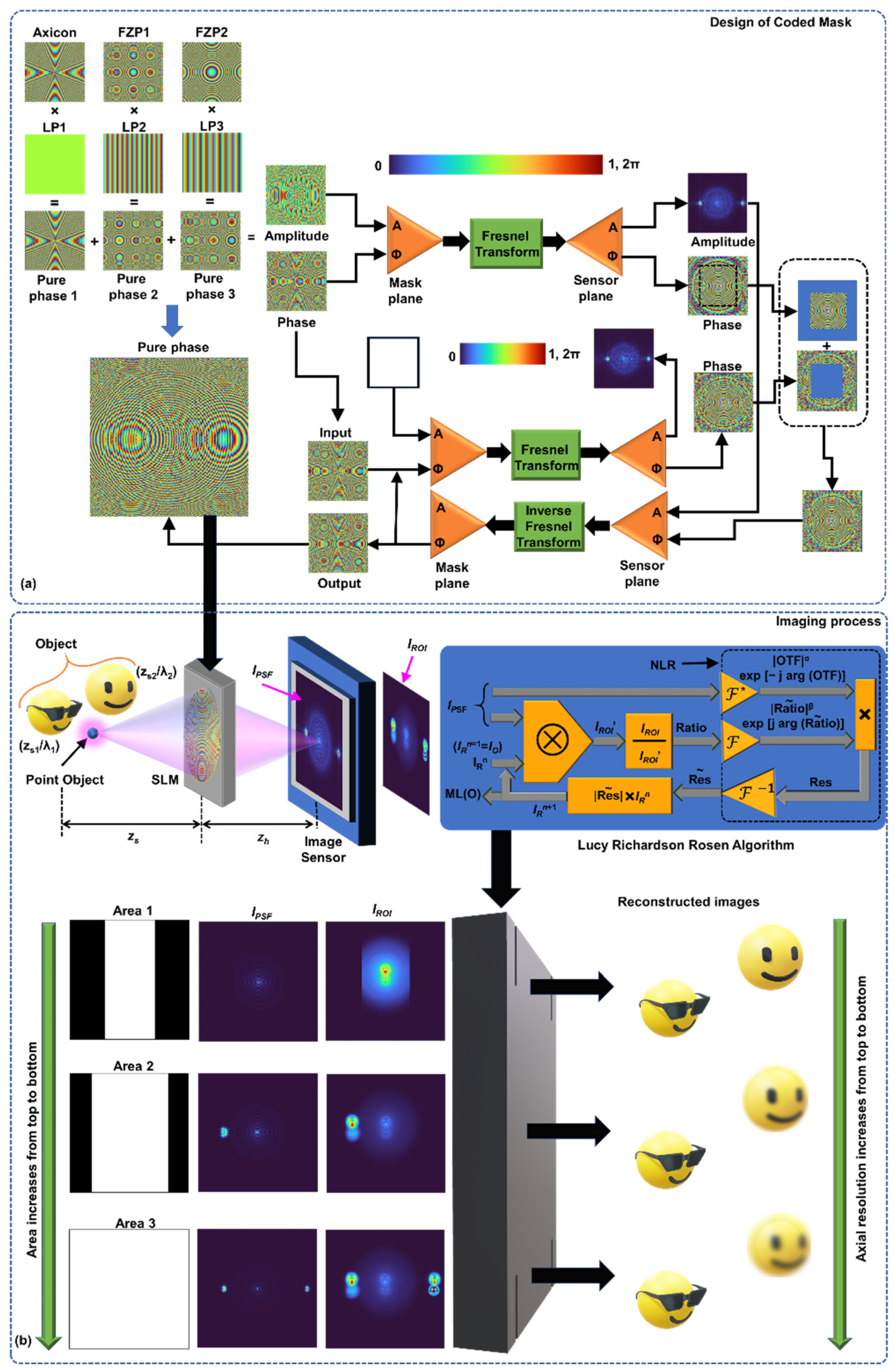
Figure 2.
Simulation results for design and analysis of CM: Phase images of (a) diffractive axicon, (b) FZP1, (c) FZP2. (d) Amplitude and (e) phase of CM. Phase images of CM designed by (f) random multiplexing and (g) TAP-GSA. Diffraction patterns obtained from (h) complex CM, (i) CM designed by random multiplexing and (j) CM designed by TAP-GSA.
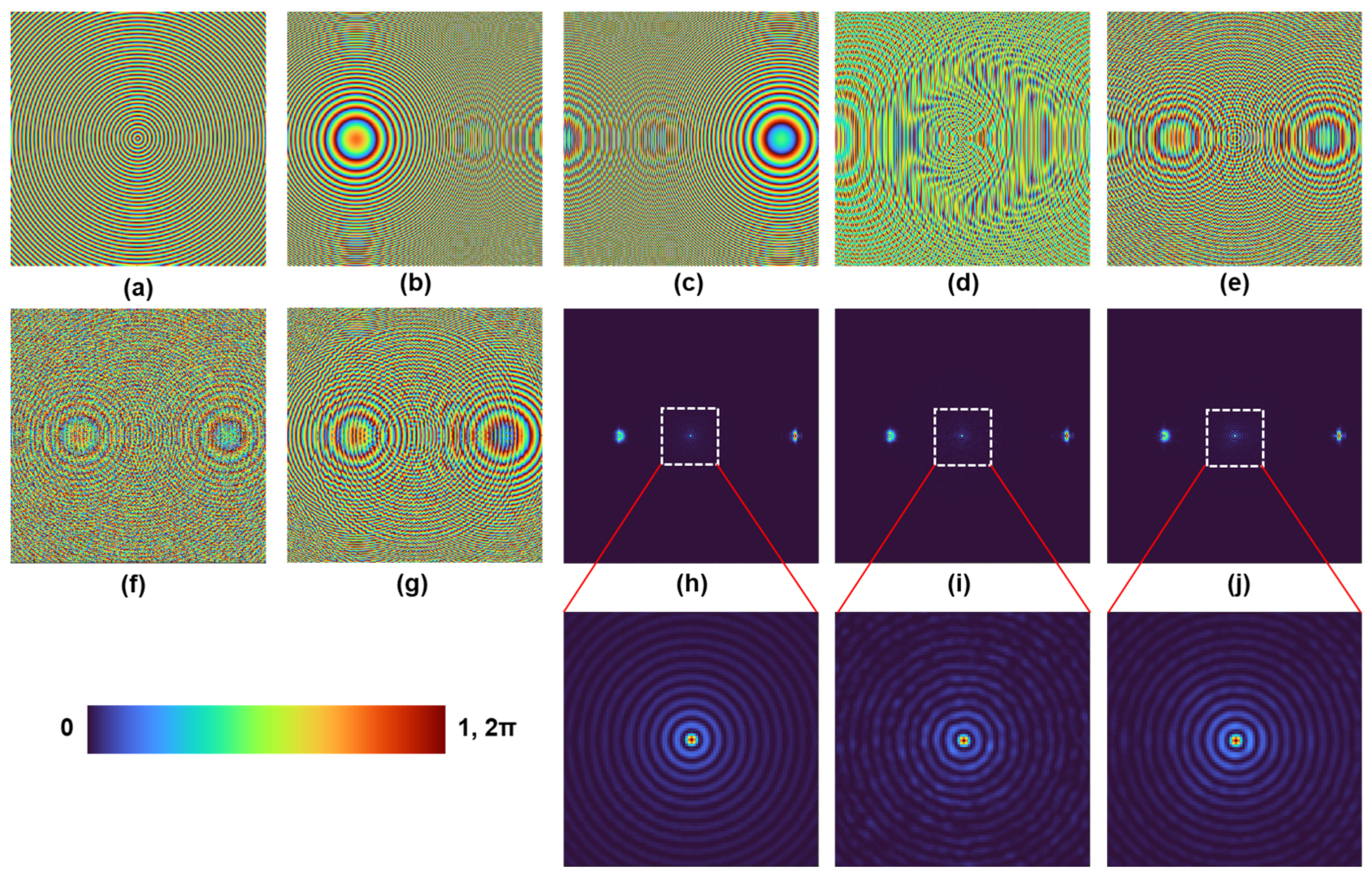
Figure 3.
Simulation results of axial correlation curves for different masks applied to the recorded IPSF and IROI. The grey region in Mask 2 has a ratio of 0.33 with the white region.
Figure 3.
Simulation results of axial correlation curves for different masks applied to the recorded IPSF and IROI. The grey region in Mask 2 has a ratio of 0.33 with the white region.
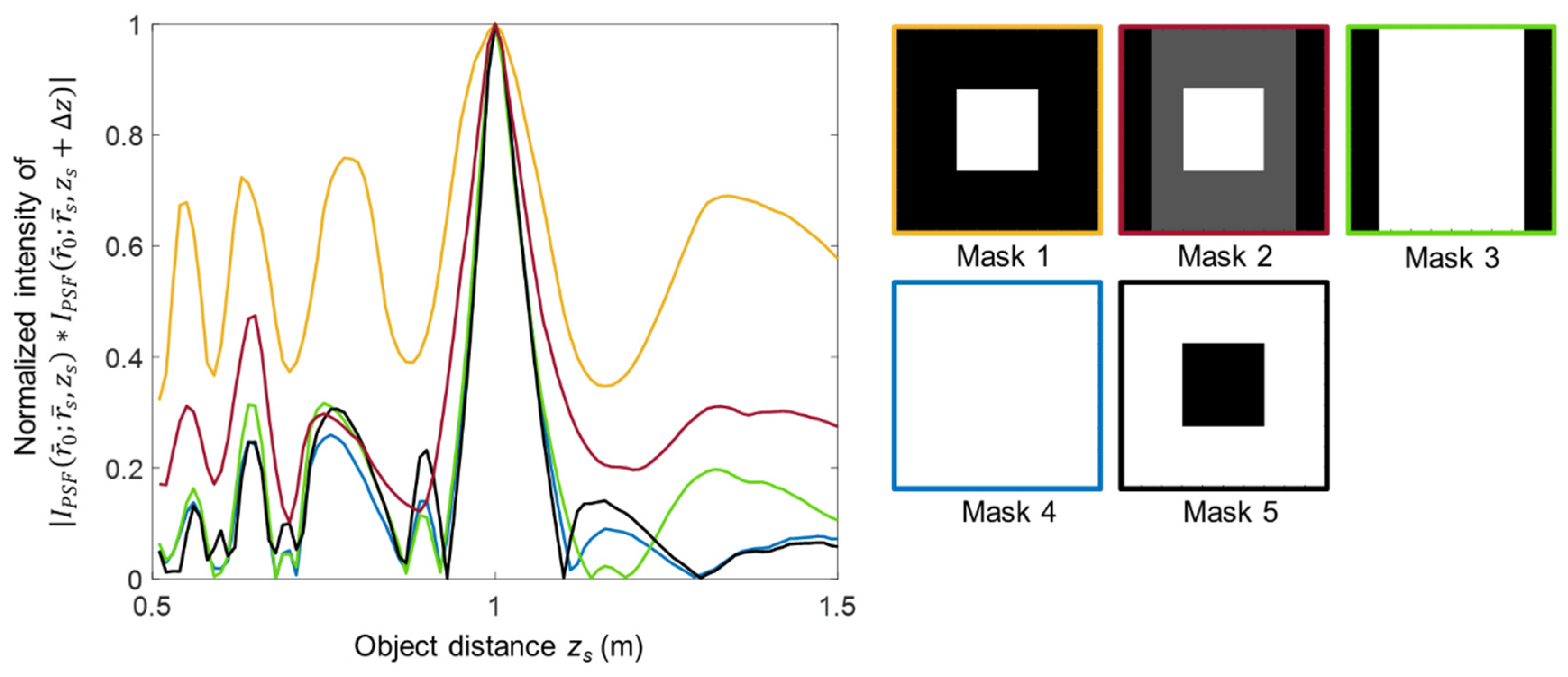
Figure 4.
(a) Test object 1, (b) Test object 2. Images of (c) IPSF (d) IROI (e) IR for Mask 1. Images of (f) IPSF (g) IROI (h) IR for Mask 2. Images of (i) IPSF (j) IROI (k) IR for Mask 4.
Figure 4.
(a) Test object 1, (b) Test object 2. Images of (c) IPSF (d) IROI (e) IR for Mask 1. Images of (f) IPSF (g) IROI (h) IR for Mask 2. Images of (i) IPSF (j) IROI (k) IR for Mask 4.
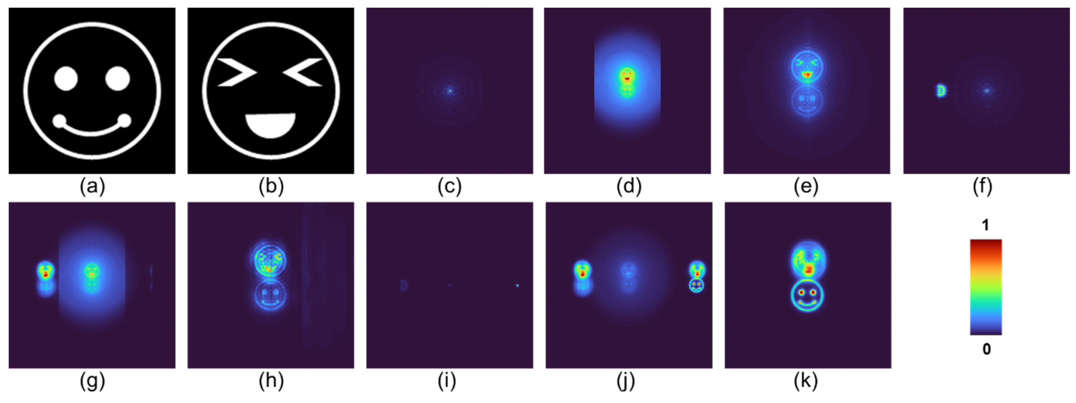
Figure 5.
(a) Schematic and (b) photograph of the experimental configuration. (1) LED, (2) iris, (3) refractive lens (f = 3.5 cm), (4) polarizer, (5) refractive lens (f = 5 cm), (6) object/pinhole, (7) refractive lens (f = 5 cm), (8) iris, (9) beam splitter, (10) spatial light modulator, (13) monochrome image sensor.
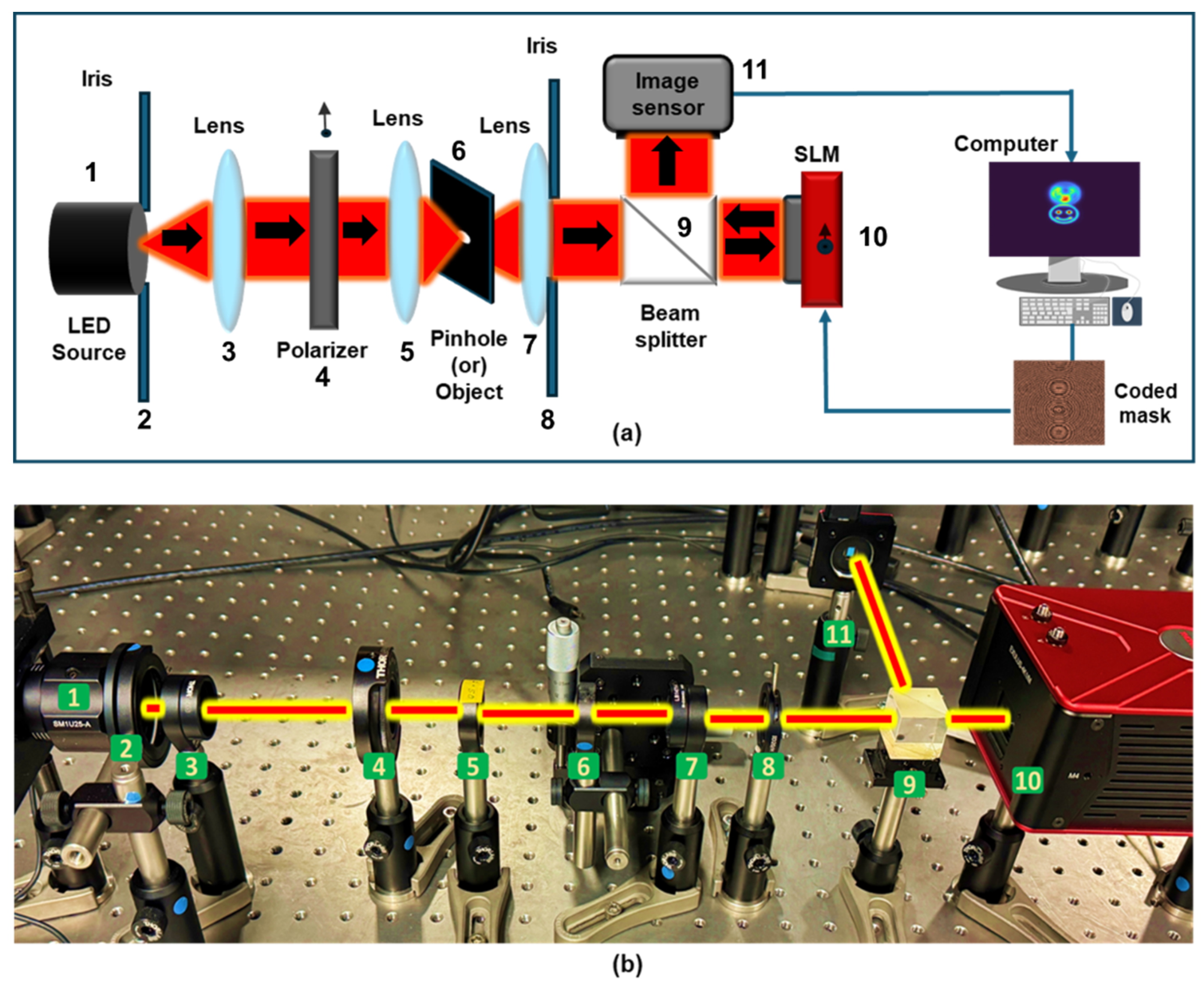
Figure 6.
Experimentally recorded (a) IPSF, (b) IROI. Images of (c) Mask1 and the (d) corresponding reconstruction. Images of (e) Mask 2 and the (f) corresponding reconstruction. (g) Phase image of the CM desiged by TAP-GSA with 75% degrees of freedom.
Figure 6.
Experimentally recorded (a) IPSF, (b) IROI. Images of (c) Mask1 and the (d) corresponding reconstruction. Images of (e) Mask 2 and the (f) corresponding reconstruction. (g) Phase image of the CM desiged by TAP-GSA with 75% degrees of freedom.
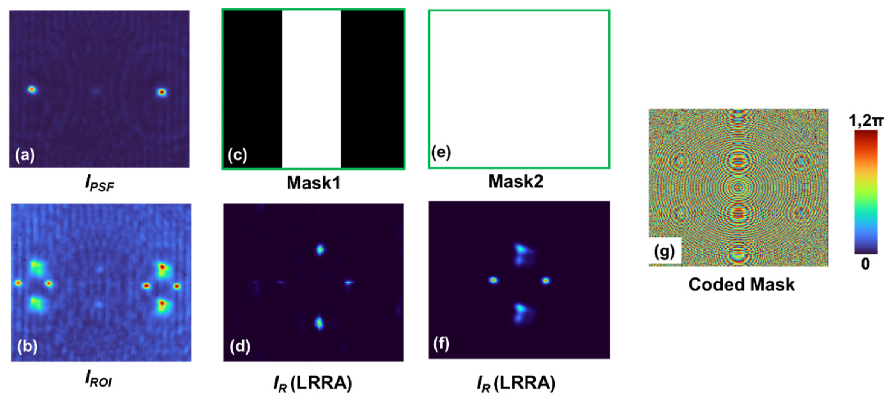
Figure 7.
Simulation results of spectral correlation curves for different masks applied to the recorded IPSF and IROI. The grey region in Mask 2 has a ratio of 0.33 with the white region.
Figure 7.
Simulation results of spectral correlation curves for different masks applied to the recorded IPSF and IROI. The grey region in Mask 2 has a ratio of 0.33 with the white region.
Disclaimer/Publisher’s Note: The statements, opinions and data contained in all publications are solely those of the individual author(s) and contributor(s) and not of MDPI and/or the editor(s). MDPI and/or the editor(s) disclaim responsibility for any injury to people or property resulting from any ideas, methods, instructions or products referred to in the content. |
© 2024 by the authors. Licensee MDPI, Basel, Switzerland. This article is an open access article distributed under the terms and conditions of the Creative Commons Attribution (CC BY) license (https://creativecommons.org/licenses/by/4.0/).
Copyright: This open access article is published under a Creative Commons CC BY 4.0 license, which permit the free download, distribution, and reuse, provided that the author and preprint are cited in any reuse.


