
Submitted:
09 November 2024
Posted:
11 November 2024
You are already at the latest version
Abstract
This work presents the design of optimal and multiplierless compensators for Chebyshev sharpened comb decimation filters. The narrowband and wideband compensators are proposed. For the narrowband, the compensator with a magnitude response is proposed in a sinusoidal form, while for the wideband, two compensators with magnitude responses of two sinusoidal functions are introduced. The optimum design is performed using particle swarm optimization (PSO), while the multiplierless design is realized by presenting optimum parameters in a signed-power-of-two (SPT) form. Unlike methods in the literature, this approach presents flexibility in design, allowing for an exchange between the quality of optimization and the complexity. Comparisons with the compensators from the literature demonstrated that the proposed method provides much better compensation while requiring fewer or slightly increased number of adders.
Keywords:
decimation
; comb
; sharpening
; Chebyshev sharpening
; compensator
; narrowband
; wideband
1. Introduction
The Kaiser-Hamming sharpening [1] of comb decimation filters was first introduced in [2] to improve the passband and stopband characteristics of the filters. Later, various improvements to the Kaiser sharpening method were presented [3,4,5,6,7]. The Chebyshev sharpening of comb decimation filters first introduced Coleman in [8]. This filter provides a high predetermined attenuation in all folding bands. However, the passband has a high passband droop. The author also proposed a pre-sharpening version in which the passband droop is decreased but still needs to be improved. The authors in [9] proposed a novel structure for Chebyshev sharpening, while in [10,11], are proposed different Chebyshev sharpening polynomials and the optimal filters to compensate for the passband droop. In [12], the method to design an optimal compensator for Chebyshev sharpening combs provides better compensation than the compensators in [11]. The method is based on particle swarm optimization (PSO) and sinusoidal magnitude response.
This paper extends the previous paper [12]. Three compensators for Chebyshev sharpened comb filters from the literature are introduced to enhance passband compensation and increase the flexibility of the design. The novelty of this work includes the following:
- Design three optimal and multipliers compensators, all with sinusoidal magnitude responses, with different complexity for the Chebyshev sharpened comb filters [8] and [10,11], providing a trade-off between the quality of compensation, the number of the required adders, and the width of the passband.
- The flexibility of the design.
The paper is organized as described in continuation. Next Section introduces three compensators of different complexity and describes the design procedure. Section 3 presents the passband compensation of the Chebyshev sharpened combs introduced in [8] and [11]. Section 4 presents the comparisons with the methods from the literature.
2. Design of Compensators
Compensators are a key area of research in the field of comb filters. They are designed to improve the passband characteristics of comb filters [13,14,15,16,17] or modified comb filters [18] at a low sample rate, i.e., after the decimation. Typically, compensators are designed as finite impulse responses (FIR) filters using various optimization methods to ensure that the cascade of the filter and the compensator provides as low as possible deviation in the passband of interest. We will adopt the denotations, as shown in the continuation.
The comb filter of order K and the decimation factor M is denoted as:
The Chebyshev sharpened comb is denoted as G(z) and the compensator as C(z).
Since the compensator works at a low rate, using the multirate identity [19] the cascade of the Chebyshev sharpened comb and compensator is given as:
Gc(z)=G(z)C(zM).
As the comb compensator introduced in [13,14,15,16] has sinusoidal magnitude characteristics while exhibiting high-quality compensation, we also propose to use the sinusoidal magnitude responses for the proposed compensators. We consider narrowband and wideband designs, as described in the following.
2.1. Narrowband Design
In this design, the passband frequency ωp <1/4M. The magnitude characteristic is chosen as in [13],
where C11 is the parameter of the design.
The system function of this filter is given as [13],
The compensator requires three adders and one multiplier. In a multiplierless design, the number of required adders equals:
where N11 is the number of adders in the signed-power-of-two (SPT) form of C11.
2.2. Wideband Design
In the wideband design the passband frequency ωp equals 1/4M≤ ≤1/2M.
We consider two sinusoidal compensators.
2.2.1. Extension of Narrowband Design
The system function of this compensator is given as:
The compensator requires nine adders and two multipliers C21 and C22. The number of the required adders in a multiplierless design is given as
where N21 and N22 are the number of adders in SPT forms of C21 and C22, respectively.
To increase the flexibility of the design, we also consider the less complex compensator from [16] introduced in the next subsection.
2.2.2. Simplified Version of Compensator in (6)
The system function is given as [16],
The compensator requires six adders and two multipliers C31 and C32. The number of the required adders in a multiplierless design is,
where N31 and N32 are the number of adders in SPT forms of C31 and C32, respectively.
2.3. How to Obtain the Compensator Design Parameters?
We first consider optimum design to get the parameters in compensators (3), (6), and (9) in a way that a minimum of the maximum passband deviation δo in the passband of interest, defined by the passband edge ωp equals
where is given in (2), and the compensators are given in (3), (6), and (9).
The optimal design is obtained using particle swarm optimization (PSO) in MATLAB [20].
3. Passband Compensation of Chebyshev Sharpened Combs from [8] and [10,11]
3.1. Coleman Chebyshev Sharpened Comb [8]
The fifth-order Chebyshev polynomial coefficients in [8] are [0,5,-20,16]. We decimation factor M=16, and the attenuation in the stopbands is -100 dB [8].
3.1.1. Narrowband Compensation
We consider ωp=0.22/M and the compensator C1 in (3). Using PSO in MATLAB, we get C11o=0.9089 resulting in the optimum passband deviation of δo=0.0141dB. Next, C11o is presented in the SPT form varying the number of adders from four to seven, as shown in Table 1. The results are shown in Table 1. It can be observed that we have approximately optimum compensation with seven adders, denoted in bold in Table 1.
Figure 1.a compares overall magnitude responses of non-compensated Coleman filter and compensated with the optimum compensator (3). The compensation slightly deteriorates the stopband, as shown in Figure 1a. Figure 1b compares passbands of the Coleman noncompensated filter, compensated with the optimum filter, and compensated with the SPT filter from Table 1with N1=5.
3.1.2. Wideband Compensation
The passband frequency ωp=1/2M, and M=16.
Compensator C2
We first consider the compensator C2 from (6). The optimal compensator coefficients are: C21o=0.7904, and C22o=0.8596, resulting in δo=0.0239 dB. The corresponding SPT coefficients are shown in Table 2. It can be observed that with fifteen adders, we have approximately optimum compensation.
Figure 2 contrasts the passband magnitude responses of the Coleman non-compensated, optimum compensated, and the SPT compensated with N2=12.
Compensator C3
The optimal compensator coefficients are C31o=0.7250 and C32o=1.3138, resulting in δo=0.045 dB. The corresponding SPT coefficients are shown in Table 3. With twelve and thirteen adders, we have approximately optimum compensation.
Figure 3 compares the Coleman non-compensated filter passbands, compensated with the optimum filter, and compensated with the SPT filter, N3=11.
3.2. Chebyshev Sharpened Comb Filters [11]
We consider M=20 and Chebyshev polynomial from [11],
where x is a comb filter (1)
p(x)=1-29x2+215x4,
3.2.1. Narrowband Compensation
We chose ωp=0.22π/M and the compensator C1 in (3). The optimum parameter C11o=0.7213, and δo=0.0111dB. The SPT coefficients are given in Table 4, changing N1 from four to eight. For N1 =8, we get approximately the optimum compensation.
3.2.2. Wideband Compensation
The passband frequency ωp = π/2M, while the decimation factor M and the Chebyshev sharpening polynomial are the same as in Section 3.2.1. We will consider the wideband compensators C2 and C3.
- Compensator C2
The optimum values of the compensator parameters obtained using the PSO method are C21o=0.6337 and C22o=0.6264, while the passband deviation equals δo=0.0171 dB. To get a multiplierless design the optimum parameter values are presented in the SPT form and the results are shown in Table 5. It can be observed that with N2=15 we can get almost optimum compensation.
Figure 5 contrasts the magnitude responses in passband of the non-compensated, optimum compensated, and the SPT compensated (N2=12) Chebyshev sharpened comb filter [11].
- Compensator C3
The optimum parameters are obtained using PSO, resulting in C21o=0.5946, C22o=0.8939, and δ2o=0.0302 dB. The SPT parameter values are given in Table 6., along with the corresponding passband deviations and the number of compensator adders.
As observed in Table 6, the approximate optimal optimization can be obtained with N3=12.
4. Results
In this section, we present the benefits of the proposed method and compare it with the methods in the literature.
4.1. Comparisons
Only a few works propose compensators for Chebyshev sharpening combs [10,11,12]. However, we also include a comparison with one of the most recent works, in which another type of sharpening is applied to improve the passband and stopband of comb filters.
4.1.1. Comparison with Method in [10]
In Table 1 [10], the authors proposed four compensated Chebyshev sharpened combs. In continuation, we then present a comparison of all the cases.
- Chebyshev sharpening polynomial p(x)=1-29x+215x2, x=H(z,1,32)
The passband edge is ωp=0.226π/M where M =32.The design in [10] requires N=9 adders, resulting in δp=0.06 dB. We used the narrowband compensator C1. The PSO design results in C11o=0.3549 and δo=0.0043 dB. The SPT design results are shown in Table 7.
The results in Table 7 highlight the efficiency of the proposed designs (denoted in bold), which outperform those in [10], requiring fewer adders and providing better compensation.
- Chebyshev sharpening polynomial p(x)=1-210x+217x2, x=H(z,1,32)
The passband edge is ωp=0.164π/M where M =32.The design in [10] requires N=8 adders, resulting in δp=0.02 dB. In the proposed design we choose the compensator C1. The optimum PSO design gives C11o =0.3443 and δo=0.0012 dB. The results of the SPT design are shown in Table 8.
The proposed designs (denoted in bold) confidently present superior compensation, requiring fewer adders.
- Chebyshev sharpening polynomial p(x)=-1+27(26x-214x2+220x3), x=H(z,1,32)
The passband frequency equals ωp=0.187π/M and M=32 resulting in N=13 adders and δp=0.05 dB in the design [10]. We applied the compensator C1 and the PSO design, obtaining C11o=0.5248 and δo=0.0034 dB. The results of the SPT design are shown in Table 9.
Once again, the proposed design shown in Table 9 reassures us with its significantly improved compensation and fewer adders.
- Chebyshev sharpening polynomial p(x)=-1+27(24x-210x2+214x3), x=H(z,1,32)
The passband edge equals ωp=0.354π/M and M=32.The design in [10] resulted in N=13 adders and δp=0.05 dB. In our design, we chose the wideband compensator C3. The PSO design results in C33o=and δo=dB, while the results of the SPT design are shown in Table 10.
In Table 10, presented in bold, the proposed design demonstrates better compensation and fewer adders in all cases.
4.1.2. Comparison with Method in [11]
The authors in [11] proposed four Chebyshev sharpened combs and the corresponding optimum compensator designs to improve the passband while keeping the number of adders as low as possible. We compare our designs, taking narrowband and wideband cases.
- Chebyshev sharpening polynomial p(x)=1-29x2+215x4, x=H(z,1,32)
The passband edge equals ωp=0.226π/M where M=32. The design in [11] requires N=3 adders resulting in δp=0.02 dB. In our design, we chose the narrowband compensator C1. The results of the PSO design are C11o=0.3543 and δ1o=0.0043 dB, while the results of the SPT design are shown in Table 11.
The proposed design in the first row of Table 11 exhibits better compensation at the expense of one additional adder. Unlike [11], the proposed design's flexibility offers further advantages and improved passband compensation by slightly increasing the adders.
- Chebyshev sharpening polynomial p(x)=-1+27(24x-210x2+214x3), x=H(z,1,32)
The passband edge equals ωp=0.483π/M and M=32.The optimum design in [11] requires N=7 adders, resulting in δp=0.12 dB. Since C3 requires fewer adders than C2, we apply the wideband compensator C3 in our design. The results of the optimal PSO design are C31o=0.8888, C32o=1.8668 and δ3o=0.0554 dB, while the SPT design results are given in Table 12.
4.1.3. Comparison with Method in [12]
We compare our design with Example 2 in [12], where the compensator for Chebyshev sharpening polynomial p(x)=-1+27(23x2-28x4+211x6), x=H(z,1,32), is designed. The design's results are given in Table II in [12]. Our design, meticulously presented in Table 13, provides a clear comparison. For N2=11, the passband deviation equals 0.0307 dB, compared to 0.0587 dB, shown in the third row of Table II in [12]. Further increase in the number of adders, a key design parameter, results in a decrease of the passband deviation, as shown in Table 13. This relationship demonstrates the design's ability to improve performance with increased complexity.
4.1.4. Comparison with Method in [7]
In [7], a two-stage comb decimation filter with a sharpened comb in the second stage was proposed. A linear optimization technique determines the coefficients of sharpening polynomial. The complexity of the design expressed in the number of adders per output sample (APOS) equals 163, while the minimum stopband attenuation is 30 dB, and the passband deviation is 0.16 dB. This work is compared in [7] with the compensated Chebyshev sharpening comb using polynomial p(x)=1-29x2+215x4 [11] for ωp=0.226π/M and M=32. This filter requires 138 APOS with a minimum stopband attenuation of 38.12 dB and a passband deviation of 0.02 dB.
4.2. Principal Features of the Proposed Method
The principal features of the proposed method to improve the passband of the Chebyshev sharpened comb filters from the literature are summarized as follows:
- The method includes the compensation of Coleman Chebyshev comb filters, which have a favorite characteristic of providing high and equal attenuations in all folding bands.
- The choice of narrowband and wideband compensators depends on the passband of interest. For the wideband case, there is a choice between two compensators depending on the number of adders and the compensation quality.
- All designs have the option of optimal multiplier and multiplierless designs.
- Design flexibility presented as a trade-off between the number of adders and the quality of compensations.
- The comparisons with the methods from the literature demonstrate the advantages of the proposed method.
References
- Kaiser, J.; Hamming, R. Sharpening the response of a symmetric nonrecursive filter by multiple use of the same filter. IEEE Trans. Acoust. Speech, Signal Process. 1977, 25, 415–422. [Google Scholar] [CrossRef]
- Kwentus, A.; Jiang, Z.; Willson, A. Application of filter sharpening to cascaded integrator-comb decimation filters. IEEE Trans. Signal Process. 1997, 45, 457–467. [Google Scholar] [CrossRef]
- Jovanovic-Dolecek, G.; Mitra, S. A new two-stage sharpened comb decimator. IEEE Trans. Circuits Syst. I: Regul. Pap. 2005, 52, 1414–1420. [Google Scholar] [CrossRef]
- Stephen, G.; Stewart, R. High-speed sharpening of decimating CIC filter. Electron. Lett. 2004, 40, 1383–1384. [Google Scholar] [CrossRef]
- Aggarwal, S. Efficient design of decimation filter using linear programming and its FPGA implementation. Integration 2021, 79, 94–106. [Google Scholar] [CrossRef]
- Aggarwal, S.; Meher, P.K. Enhanced Sharpening of CIC Decimation Filters, Implementation and Applications. Circuits, Syst. Signal Process. 2022, 41, 4581–4603. [Google Scholar] [CrossRef]
- Gautam, D.; Khare, K.; Shrivastava, B.P. A Novel Approach for Optimal Design of Sample Rate Conversion Filter Using Linear Optimization Technique. IEEE Access 2021, 9, 44436–44441. [Google Scholar] [CrossRef]
- Coleman, J.O. Chebyshev Stopbands for CIC Decimation Filters and CIC-Implemented Array Tapers in 1D and 2D. IEEE Trans. Circuits Syst. I: Regul. Pap. 2012, 59, 2956–2968. [Google Scholar] [CrossRef]
- Troncoso Romero, D.E. Jovanovic Dolecek, G. In and Laddomada, M. Efficient design of two-stage comb-based decimation filters using Chebyshev sharpening. In Proceedings of the 2013 IEEE 56th International Midwest Symposium on Circuits and Systems (MWSCAS), Columbus OH, USA, 04-07 August 2013. [Google Scholar]
- Molnar, G.; Dudarin, A.; Vucic, M. Design and Multiplierless Realization of Maximally Flat Sharpened-CIC Compensators. IEEE Trans. Circuits Syst. II: Express Briefs 2017, 65, 51–55. [Google Scholar] [CrossRef]
- Dudarin, A.; Molnar, G.; Vucic, M. Optimum multiplierless compensators for sharpened cascaded-integrator-comb decimation filters. Electron. Lett. 2018, 54, 971–972. [Google Scholar] [CrossRef]
- Dolecek, G.J.; Novelo, G.M. Design of compensator for Chebyshev sharpened comb filter. In Proceedings of the 2023 IEEE 33rd International Conference on Microelectronics (MIEL), Nis, Serbia, 6-18 October 2023. [CrossRef]
- Dolecek, G.J.; Fernandez-Vazquez, A. Trigonometrical approach to design a simple wideband comb compensator. AEU - Int. J. Electron. Commun. 2014, 68, 437–441. [Google Scholar] [CrossRef]
- Dolecek, G.J.; Baez, R.G.; Salgado, G.M.; de la Rosa, J.M. Novel Multiplierless Wideband Comb Compensator with High Compensation Capability. Circuits, Syst. Signal Process. 2016, 36, 2031–2049. [Google Scholar] [CrossRef]
- Salguero-Luna, S. and Jovanovic Dolecek, G. Increasing the flexibility of comb compensator design using particle swarm optimization. Ing Invest y Tecn, 2021.Volume XXII, pp. 1-12. (in Spanish).
- Dolecek, G.J.; de la Rosa, J.M. Design of wideband comb compensator based on magnitude response using two sinusoidals and particle swarm optimization. AEU - Int. J. Electron. Commun. 2020, 130, 153570. [Google Scholar] [CrossRef]
- Xu, L.; Yang, W.; Tian, H. Design of Wideband CIC Compensator Based on Particle Swarm Optimization. Circuits, Syst. Signal Process. 2018, 38, 1833–1846. [Google Scholar] [CrossRef]
- Dolecek, G.J. Comb decimator design based on symmetric polynomials with roots on the unit circle: Two-stage multiplierless design and improved magnitude characteristic. Int. J. Circuit Theory Appl. 2022, 50, 2210–2227. [Google Scholar] [CrossRef]
- Harris, F.J. Multirate Signal Processing for Communication Systems; Taylor & Francis: London, United Kingdom, 2022. [Google Scholar]
- https://www.mathworks.com/help/gads/particleswarm.html. Accessed: Sept 15, 2024.
Figure 1.
Compensation with the narrowband filter C1. Overall magnitude responses and passband zooms: (a) Overall magnitude responses of Coleman non-compensated and optimal compensated filters; (b) Passband zoom od Coleman non-compensated, optimal compensated, and SPT compensated filters with N1=5.
Figure 1.
Compensation with the narrowband filter C1. Overall magnitude responses and passband zooms: (a) Overall magnitude responses of Coleman non-compensated and optimal compensated filters; (b) Passband zoom od Coleman non-compensated, optimal compensated, and SPT compensated filters with N1=5.
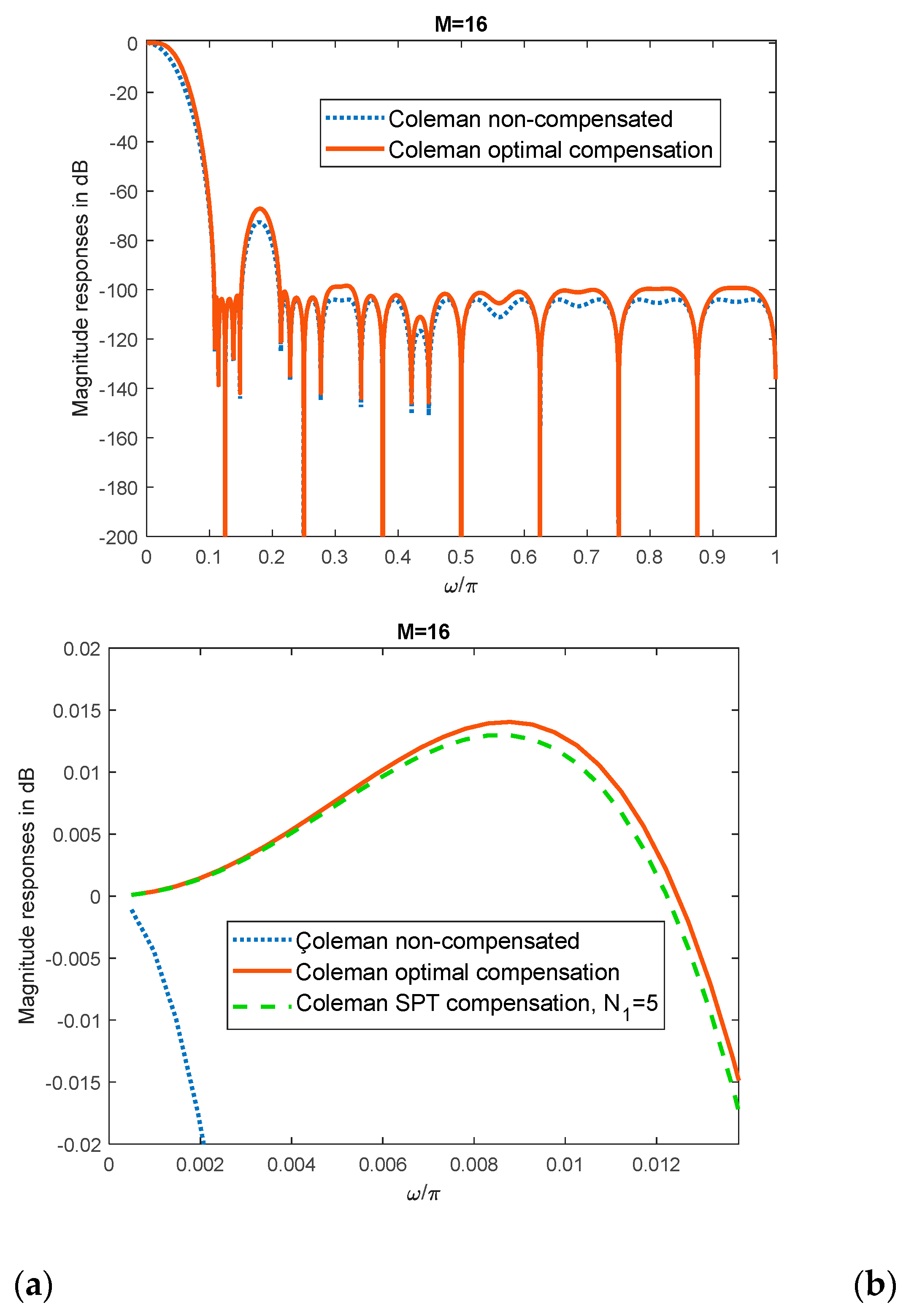
Figure 2.
Compensation with the wideband filter C2. Passband magnitude responses of non-compensated, optimal compensated, and SPT compensated Coleman sharpening comb filters with N2=12.
Figure 2.
Compensation with the wideband filter C2. Passband magnitude responses of non-compensated, optimal compensated, and SPT compensated Coleman sharpening comb filters with N2=12.
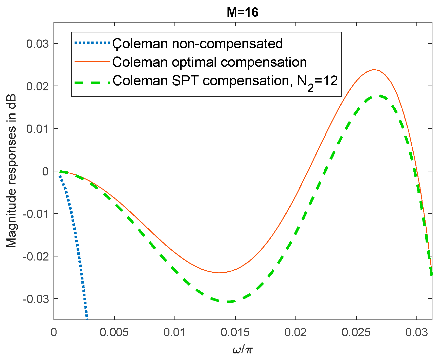
Figure 3.
Compensation with the wideband filter C3. Passband magnitude responses of non-compensated, optimal compensated, and SPT compensated Coleman sharpening comb filters, with N3=11.
Figure 3.
Compensation with the wideband filter C3. Passband magnitude responses of non-compensated, optimal compensated, and SPT compensated Coleman sharpening comb filters, with N3=11.
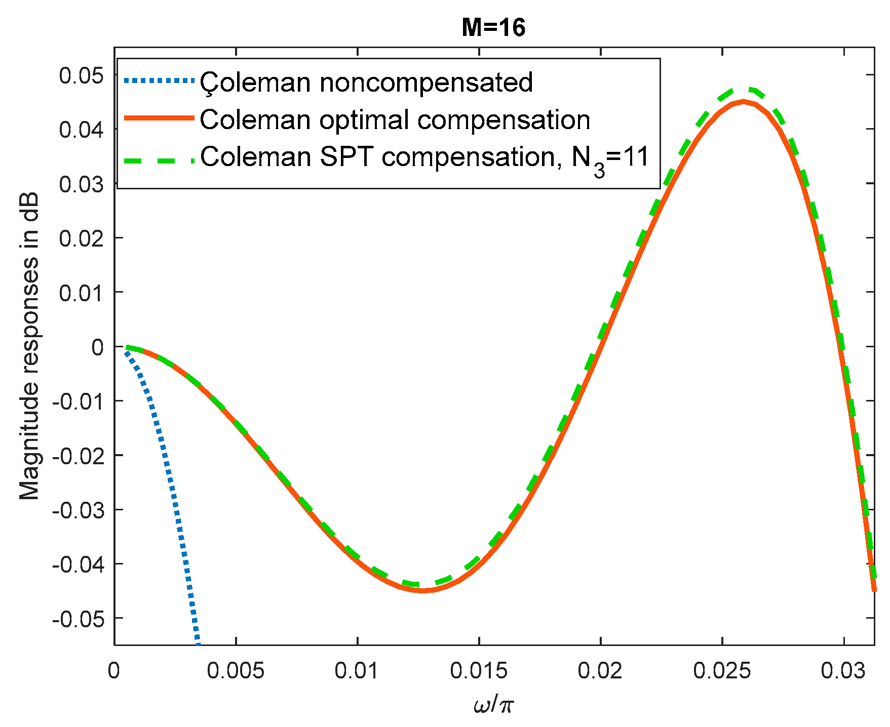
Figure 4.
Compensation with the narrowband filter C1. Passband magnitude responses of non-compensated, optimal compensated, and SPT compensated, N1=4, Chebyshev sharpening comb filters.
Figure 4.
Compensation with the narrowband filter C1. Passband magnitude responses of non-compensated, optimal compensated, and SPT compensated, N1=4, Chebyshev sharpening comb filters.
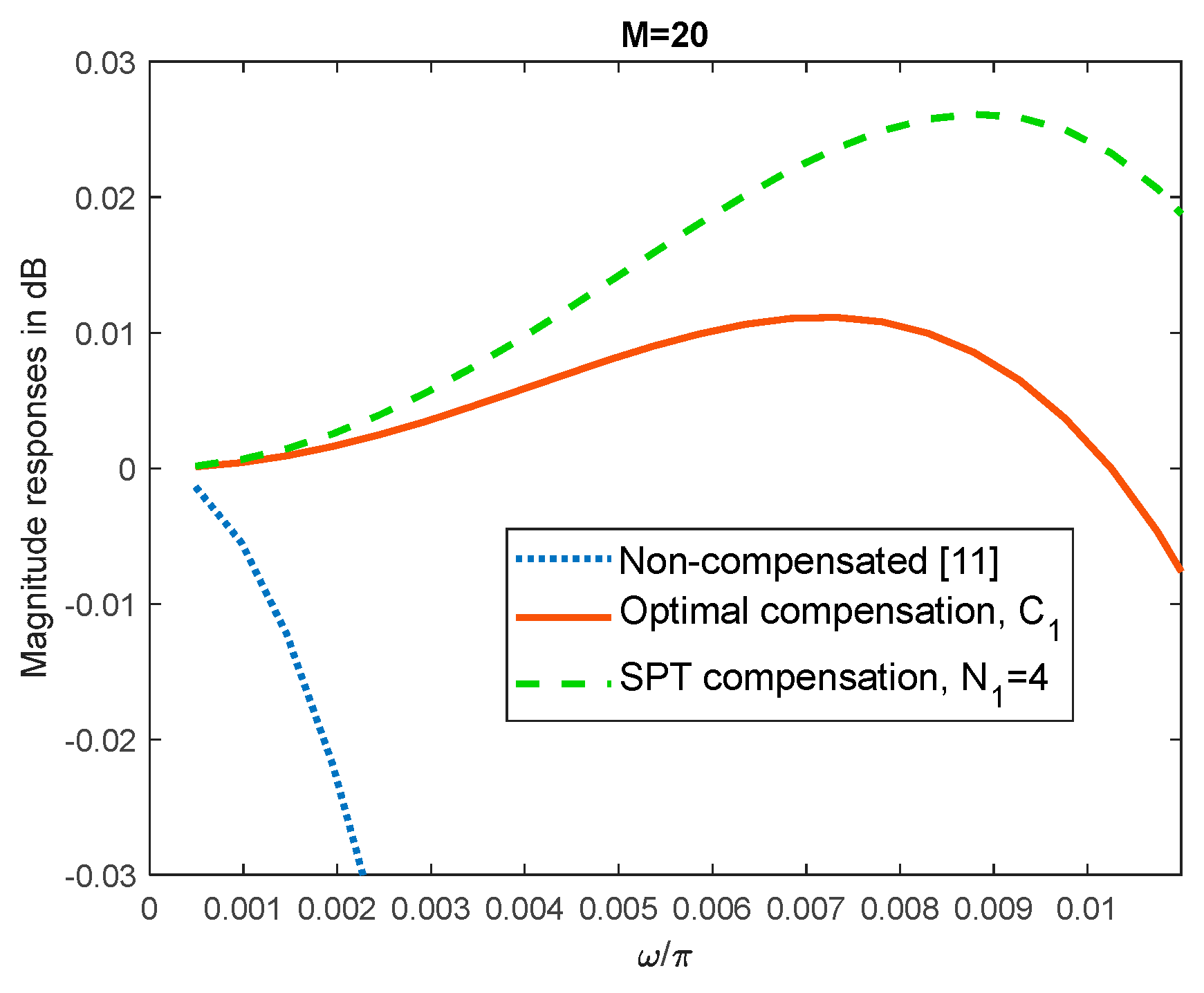
Figure 5.
Compensation with the wideband filter C2. Passband magnitude responses of non-compensated, optimal compensated, and SPT compensated, N1=4, Chebyshev sharpening comb filters.
Figure 5.
Compensation with the wideband filter C2. Passband magnitude responses of non-compensated, optimal compensated, and SPT compensated, N1=4, Chebyshev sharpening comb filters.
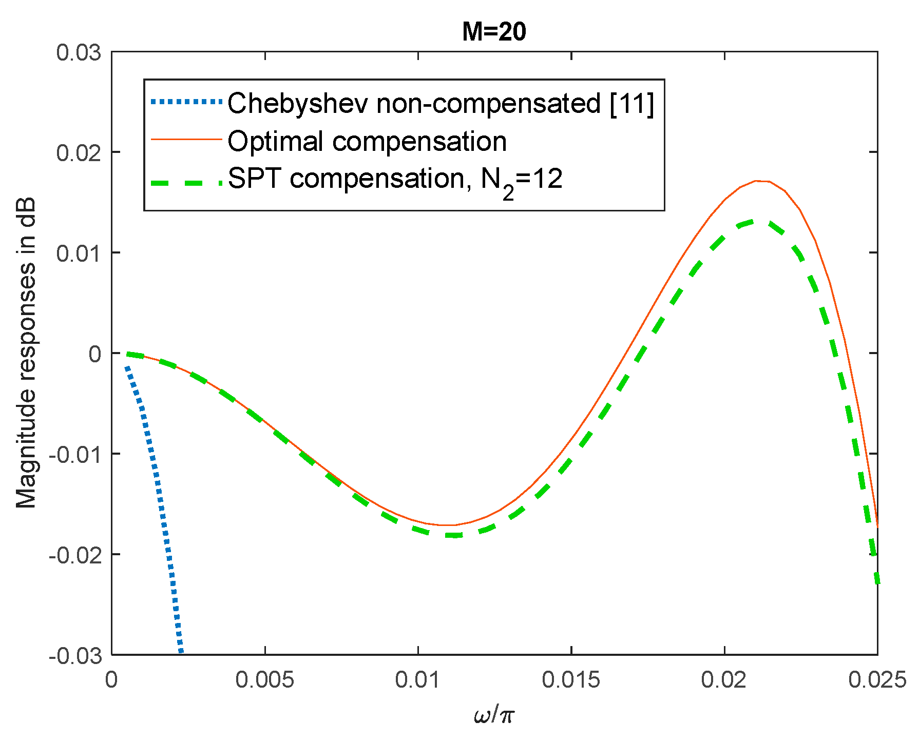
Figure 6.
Compensation with the wideband filter C3. Passband magnitude responses of non-compensated, optimal compensated, and SPT compensated, N1=4, Chebyshev sharpening comb filters.
Figure 6.
Compensation with the wideband filter C3. Passband magnitude responses of non-compensated, optimal compensated, and SPT compensated, N1=4, Chebyshev sharpening comb filters.
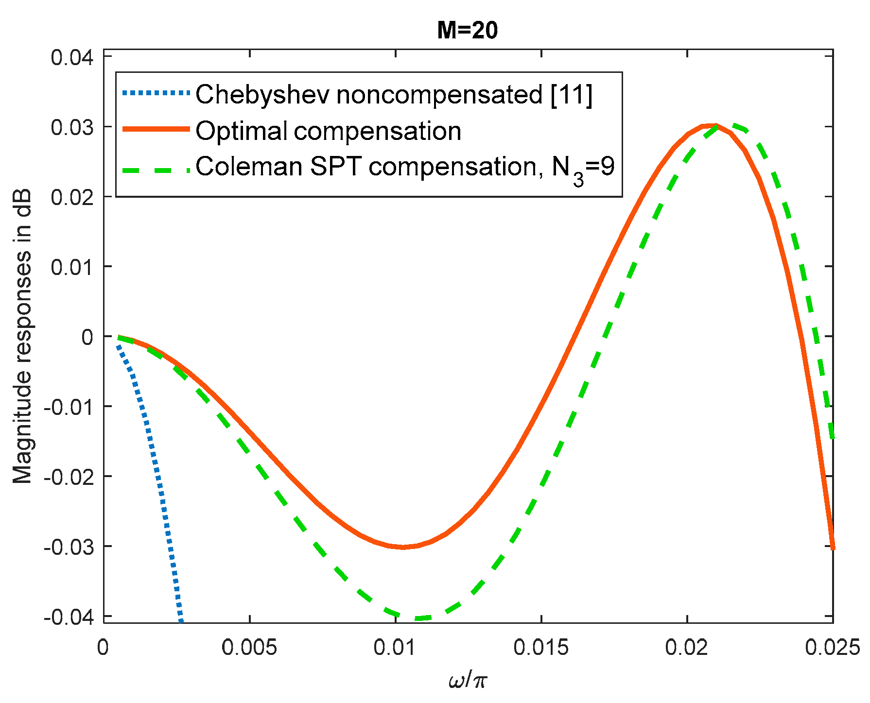

Table 1.
SPT compensator C1 coefficients, passband deviation, and the number of adders.
| C11 | δ1 [dB] | N1 |
| 20-2-4 | 0.0274 | 4 |
| 20-2-3+2-5 | 0.0165 | 5 |
| 20-2-3+2-5+2-8 | 0.0145 | 6 |
| 20-2-3+2-5+2-8-2-10 | 0.0142 | 7 |
Table 2.
SPT compensator C2 coefficients, passband deviations, and the number of adders.
| C21 | C22 | δ2 [dB] | N2 | ||
| 20-2-2 | 20-2-3 | 0.1232 | 11 | ||
| 20-2-2+2-5 | 20-2-3 | 0.0307 | 12 | ||
| 20-2-2+2-5 | 20-2-3+2-7 | 0.0297 | 13 | ||
| 20-2-2+2-5+2-8 | 20-2-3-2-10 | 0.0271 | 14 | ||
| 20-2-2+2-5+2-7 | 20-2-3-2-6+2-8 | 0.0247 | 15 |
Table 3.
SPT compensator C3 coefficients, passband deviations, and the number of adders.
| C31 | C32 | δ3 [dB] | N3 | ||
| 20-2-2 | 20-2-2+2-6 | 0.0616 | 9 | ||
| 20-2-2-2-8 | 20-2-2+2-6 | 0.0532 | 10 | ||
| 20-2-2-2-5+2-7 | 20+2-2+2-4 | 0.0474 | 11 | ||
| 20-2-2-2-5+2-7 | 20+2-2+2-4-2-9 | 0.04591 | 12 | ||
| 20-2-2-2-5+2-7-2-10 | 20-2-2+2-4-2-14 | 0.0452 | 13 |
Table 4.
SPT compensator C1 coefficients, passband deviation and the number of adders.
| C11 | δ1 [dB] | N1 |
| 20-2-2 | 0.0299 | 4 |
| 20-2-2-2-5 | 0.0125 | 6 |
| 20-2-2-2-5-2-8 | 0.0115 | 7 |
| 20-2-2-2-5-2-8+2-11 | 0.0110 | 8 |
Table 5.
SPT compensator C2 coefficients, passband deviations, and the number of adders.
| C21 | C22 | δ2 [dB] | N2 | ||
| 2-1+2--3 | 2-1+2-3 | 0.0485 | 11 | ||
| 2-1+2-3+2-7 | 2-1+2-3 | 0.0227 | 12 | ||
| 2-1+2-3+2-7 | 2-1+2-3+2-8 | 0.00177 | 13 | ||
| 2-1+2-3+2-7+2-11 | 2-1+2-3+2-9 | 0.0174 | 14 | ||
| 2-1+2-3+2-7+2-10 | 2-1+2-3+2-10+2-12 | 0.0172 | 15 |
Table 6.
SPT compensator C3 coefficients, passband deviations, and the number of adders.
| C31 | C32 | δ3 [dB] | N | ||
| 2-1-2-4 | 20-2-4 | 0.0597 | 8 | ||
| 2-1+2-4-2-6 | 20-2-4 | 0.0404 | 9 | ||
| 2-1+2-3+2-6 | 20-2-3-2-6 | 0.0373 | 10 | ||
| 2-1+2-3-2-5+2-9 | 20-2-3+2-6 | 0.0317 | 11 | ||
| 2-1+2-3-2-5+2-11 | 20-2-3+2-6+2-8 | 0.0304 | 12 |
Table 7.
SPT compensator C1 coefficients, passband deviation, and the number of adders.
| C11 | δ1 [dB] | N1 |
| 2-1-2-3 | 0.0169 | 4 |
| 2-1-2-3-2-6 | 0.0064 | 5 |
| 2-1-2-3-2-6-2-8 | 0.0045 | 6 |
| 2-1-2-3-2-6-2-8-2-11 | 0.0043 | 7 |
Table 8.
SPT compensator C1 coefficients, passband deviation, and the number of adders.
| C11 | δ1 [dB] | N1 |
| 2-1-2-3 | 0.0157 | 4 |
| 2-1-2-3-2-5 | 0.0015 | 5 |
| 2-1-2-3-2-5-2-11 | 0.0012 | 6 |
Table 9.
SPT compensator C1 coefficients, passband deviation, and the number of adders.
| C11 | δ1 [dB] | N1 |
| 2-1+2-5 | 0.0056 | 4 |
| 2-1+2-5-2-8 | 0.0042 | 5 |
| 2-1+2-5-2-7+2-9 | 0.0036 | 6 |
| 2-1+2-5-2-7+2-9-2-11 | 0.0035 | 7 |
Table 10.
SPT compensator C3 coefficients, passband deviations, and the number of adders.
| C31 | C32 | δ3 [dB] | N3 | ||
| 2-1-2-13 | 2-1-2-4 | 0.0101 | 8 | ||
| 2-1-2-13-2-16 | 2-1-2-4 | 0.0100 | 9 | ||
| 2-1-2-11-2-13 | 2-1-2-4+2-10 | 0.0098 | 10 |
Table 11.
SPT compensator C1 coefficient, passband deviations and the number of adders.
| C11 | δ1 [dB] | N1 |
| 2-1-2-3 | 0.0169 | 4 |
| 2-1-2-3-2-6 | 0.0064 | 5 |
| 2-1-2-3-2-6-2-8 | 0.0045 | 6 |
| 2-1-2-3-2-6-2-8-2-11 | 0.0043 | 7 |
Table 12.
SPT compensator C3 coefficients, passband deviations, and the number of adders.
| C31 | C32 | δ3 [dB] | N3 | ||
| 20-2-3 | 21-2-3 | 0.0776 | 8 | ||
| 20-2-3+2-7 | 21-2-3 | 0.0601 | 9 | ||
| 20-2-3+2-6-2-9 | 21-2-3-2-7 | 0.0587 | 10 | ||
| 20-2-3+2-6+2-9 | 21-2-2+2-4+2-7 | 0.0555 | 11 |
Table 13.
SPT compensator C2 coefficients, passband deviations, and the number of adders.
| C21 | C22 | δ2 [dB] | N2 | ||
| 2-1+2--5 | 2-2+2-6 | 0.0307 | 11 | ||
| 2-1-2--5+2-8 | 2-1+2-7 | 0.0276 | 12 | ||
| 2-1-2--5+2-8 | 2-1+2-7+2-9 | 0.0273 | 13 | ||
| 2-1-2--5+2-8+2-10 | 2-1+2-7-2-11 | 0.0266 | 14 | ||
| 2-1+2-5+2-7-2-9-2-11 | 2-1+2-7-2-9+2-11 | 0.0262 | 16 |
Disclaimer/Publisher’s Note: The statements, opinions and data contained in all publications are solely those of the individual author(s) and contributor(s) and not of MDPI and/or the editor(s). MDPI and/or the editor(s) disclaim responsibility for any injury to people or property resulting from any ideas, methods, instructions or products referred to in the content. |
© 2024 by the authors. Licensee MDPI, Basel, Switzerland. This article is an open access article distributed under the terms and conditions of the Creative Commons Attribution (CC BY) license (https://creativecommons.org/licenses/by/4.0/).
Copyright: This open access article is published under a Creative Commons CC BY 4.0 license, which permit the free download, distribution, and reuse, provided that the author and preprint are cited in any reuse.


