
Submitted:
04 April 2025
Posted:
07 April 2025
You are already at the latest version
Abstract
In this work, we develop a method of rational approximation of the Fourier transform (FT) based on the real and imaginary parts of the complex error function
\[
w(z) = e^{-z^2}(1 - {\rm{erf}}(-iz)) = K(x,y) + iL(x,y), \quad z = x + iy,
\]
where $K(x,y)$ and $L(x,y)$ are known as the Voigt and imaginary Voigt functions, respectively. In contrast to our previous rational approximation of the FT, the expansion coefficients in this method are not dependent on values of a sampled function. As a set of the Voigt/complex error function values remains the same, this approach provides rapid computation. Mathematica codes with some examples are presented.
Keywords:
rational approximation
; Fourier transform
; Voigt function
; complex error function
1. Introduction
The forward and inverse Fourier transforms (FTs) can be defined in a symmetric form as [1,2]
and
respectively. In this work we will consider only the forward FT (1) since due to symmetric form the approximations for the inverse FT (2) can be readily obtained from the forward FT by change of the variables.
There are relations between a function and its even and odd components. In particular, the even and odd functions can be readily generated by using the following relations
and
such that
Therefore, due to linearity of the FT we can also state that
Since an even function satisfies the condition
it follows that
and
Since an odd function satisfies the condition
we have
and
Equations (9) and (10) are of the primary importance since they will be used in derivation of the new approximation of the FT.
In our recent publication we developed a new methodology providing a rational approximation of the FT [3]. Specifically, the FT of a function can be approximated as a rational function consisting of low-order polynomials, , in form
where expansion coefficients are given by
Some examples of rational approximation (11) of the FT are shown in our work [3] and can be visualized by running a provided Matlab code 1.
There are many methods for rational approximations such as Padé approximation [4,5], minimax approximation [6,7], Remez algorithm [8,9] and so on. However, to the best of our knowledge, a method of rational approximation that we developed in [3] is new and has been reported in scientific literature.
It should be noted that in our previous publication [10], we de facto applied a rational approximation of the FT. Therefore, a new method of rational approximation, described in our paper [3], is just a generalization of a sampling and integration technique that we proposed earlier in [10] to derive rapid and high-accuracy rational approximations of the complex error function.
The small order polynomials in quotients of rational approximation (11) may be advantageous for numerical analysis with any kind of computations including matrix manipulations, integrations and differentiations. However, the rational approximation (11) requires re-computation of the four expansion coefficients , , , every time when the sampled function changes. In this work, we propose a new method of rational approximation of the FT based on a sum of the real and imaginary parts of the complex error function [11,12,13]. Such a representation of rational approximation of the FT does not require re-computation when shape of the sampled function changes.
2. Preliminaries
The complex error function, also commonly known as the Faddeeva function, can be defined as [13,14]
where . Comparing equation (12) with definition of the error function [11]
one can see that the complex error function can be expressed as [11,15]
Therefore, the complex error function can be considered as a reformulation of the error function .
Complex error function satisfies the following relation
It can be shown that the complex error function is a solution of the following differential equation
with initial condition
There is a direct relationship between these two functions. In particular, both functions are equal to each other on the upper half of the complex plane [12,13]
Separating the real and imaginary parts of the complex probability function (15) as
results in
and
respectively.
The real part of the complex probability function is known as the Voigt function that is widely used in Atmospheric Physics to describe absorption and emission of atmospheric molecules [16,17,18].
The imaginary part is also used in various fields of Physics and Engineering [19,20]. It does not have a specific name. However, following Zaghloul and Ali [15], for the convenience we will also refer to the function as the imaginary Voigt function.
It is not difficult to show that substituting the following identity [12]
into equation (16), we obtain [12,21]
and since
we can write
Sum of the equations above in terms of the real and imaginary parts yields [21]
We can see now that this equation is consistent with equation (13) of the complex error function .
3. Results and Discussion
3.1. Methodology
Consider the rectangular function (solitary rectangular function) that can be defined as
This function can be expressed by the following limit
Consequently, we can approximate the rectangular function by taking sufficiently large value of the parameter k.
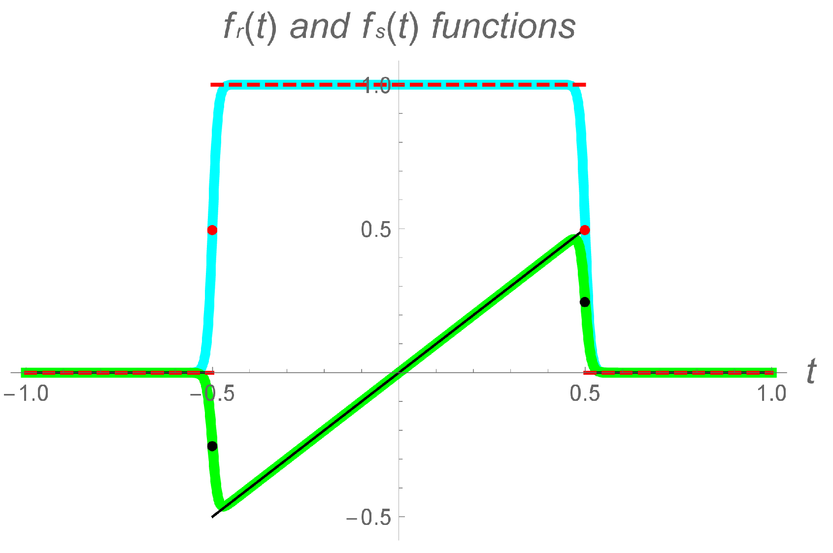
Figure 1 shows the rectangular function and its approximation at by dashed red and light blue colors, respectively. As we can see, at equation (21) approximates the rectangular function reasonably well. Therefore, we can use the following approximation
and apply it to perform numerically the FT.
Figure 1.
Rectangular and sawtooth functions and their approximations. Rectangular and sawtooth functions are shown by dashed red and solid black lines. Even and odd functions are shown by blue and green curves.
Figure 1.
Rectangular and sawtooth functions and their approximations. Rectangular and sawtooth functions are shown by dashed red and solid black lines. Even and odd functions are shown by blue and green curves.
Previously, we have used the following sampling function
where h and c are small fitting parameters, for high-accuracy approximation of the complex error function [22]. Thus, applying this sampling function over the points to approximation (22), the rectangular function can be approximated as
Figure 2 shows the approximations of the rectangular function at different fitting parameters h and c. Specifically, the green curve corresponds to , and , the red curve corresponds to , and while the light blue curve corresponds to , and . The rectangular function is also shown by black dashed curve.
Since the rectangular function is even, we can use equation (9) for the FT. Thus, the substitution of approximation (23) into equation (9) leads to
Comparing now approximation above with equation (19), one can see that the FT of the rectangular function (21) can be expressed in terms of the Voigt function
As a simplest example for an odd function, we can consider the sawtooth function (solitary sawtooth function)
Since this function can be express though the following limit
we can approximate it by multiplying t with equation (22) as follows
Figure 1 shows the sawtooth function (25) and its approximation (26) by black and light green curves, respectively.
Applying the sampling function over the points to approximation (26), we obtain
Consequently, the FT of the sawtooth function (25) can be approximated as
Comparing this equation with the imaginary Voigt function (20), we can rearrange equation above as
The applied methodology for the FTs of the rectangular and sawtooth functions (24) and (27) can be generalized to any even or odd functions as
and
Due to symmetric properties of the even and odd functions (see equations (7) and (8)), the number of the summation terms in these approximations can be reduced by a factor of two.
Let us rearrange equation (28) in the following form
Change of summation index as
leads to
Equation (29) can be expanded as
Taking into consideration that
such that according to (8)
and since
we can recast equation (32) as given by
or
or
where
At first glance the FT formulas (30) and (33) may appear computationally costly as they require user defined (external) function files. However, unlike equation (11), the expansion coefficients and , shown by equations (31) and (34), respectively, do not require re-computations every time when we change the sampled function to any other function. This gives a significant advantage. Since the values and remain always the same regardless the shape of the sampled function, these values can be precomputed in form of the look-up tables. Such implementation makes computation rapid as the required values and can be instantly picked up from the computer memory during computation of the FT. Furthermore, many algorithms, based on rational approximations, have been developed for rapid and high-accuracy computation of the Voigt/complex error function [23,24,25,26,27,28,29,30,31,32,33]. Therefore, the proposed technique can also be used as an alternative for rational approximation (11) of the FT.
3.2. Numerical Results
The FT of the rectangular function can be readily found by integration as
where
is the sinc function [34,35]. Similarly, we can find the FT of the sawtooth function as follows
We can use these analytical results for comparison with numerical FTs computed by using equations (30) and (33).
Figure 3 shows numerical FTs of rectangular and the sawtooth functions by light green and magenta curves, respectively. Equations (35) and (36) are also shown by dashed black curves.
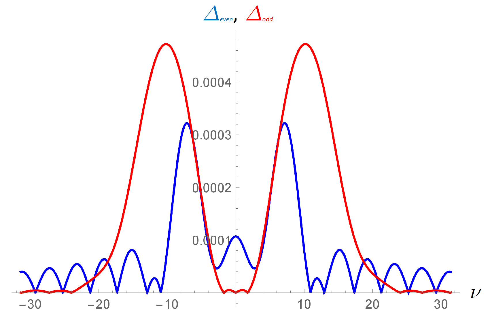
Figure 4 illustrates the absolute differences and between equations (35), (36) and numerical FT approximations (30) and (33) at , and by blue and red curves, respectively. As we can see, despite abrupt behavior of the rectangular and sawtooth functions and at and , the FT approximations (24) and (27) can provide reasonable accuracies.
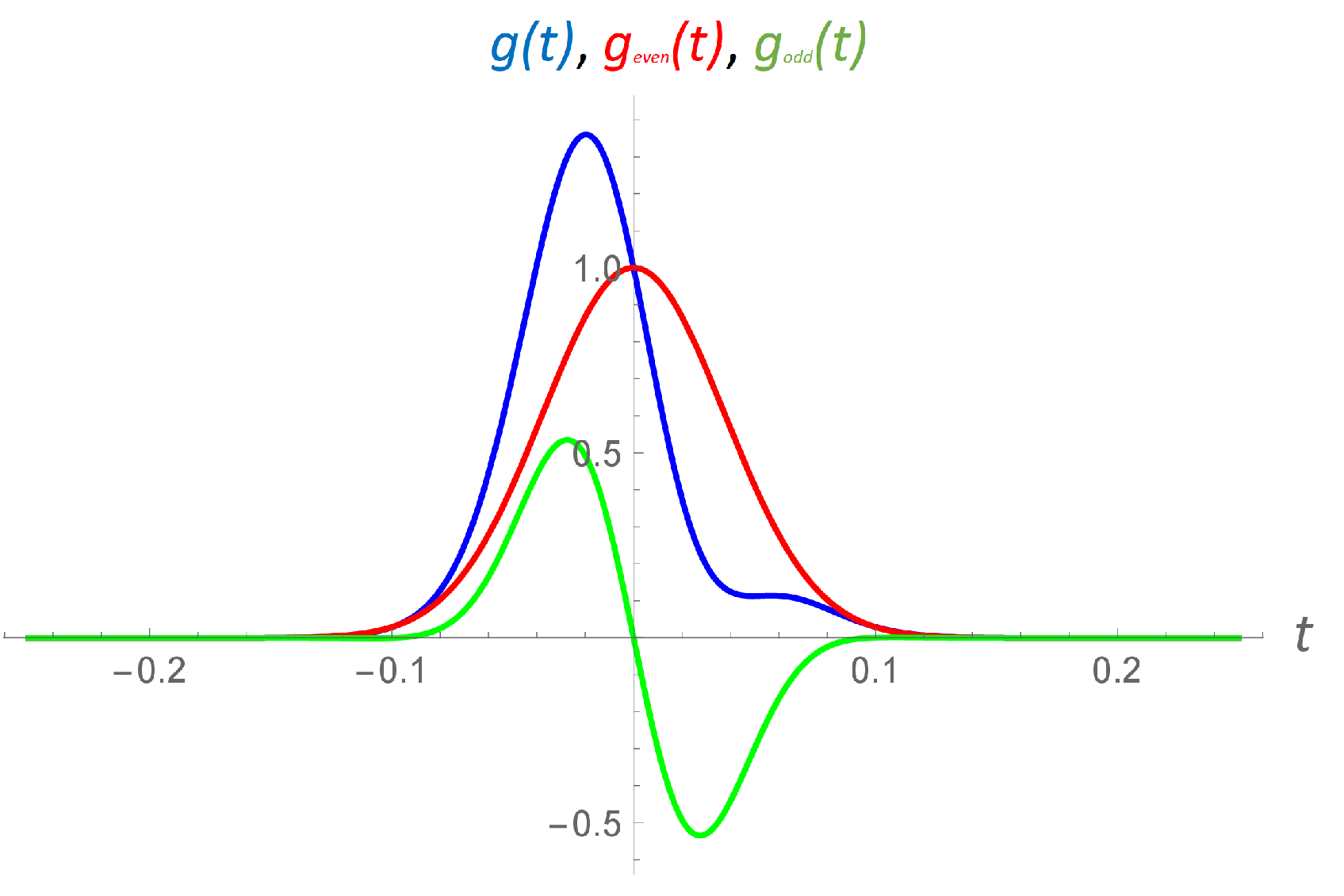
The accuracy of the FT can be significantly better for the well-behaved functions. As an example, consider a function
The first term of this function is even
while its second term is odd
Figure 5 shows the functions , and by blue, red and green colors, respectively.
3.3. Trigonometric Forms
As it has been mentioned above, the equations (28), (29) and their variations (30), (33) can be used to implement a rational approximation of the FT. We can also show how to represent these equations in trigonometric forms.
The real part of equation (14) gives
The imaginary part of equation (14) provides
Substituting this equation into approximation (34) yields
This results in
according to equation (33).
As we can see, equations (42) and (43) represent trigonometric versions of the equations (30) and (33), respectively. Despite trigonometric representations, equations (42) and (43) do not have any advantage over equations (30) and (33) in computational speed since all required values and can be precomputed and saved in a computer memory in form of the look-up tables.
We can see that equation (44) resembles the discrete Fourier transfer (DFT) [1,2]. However, unlike the DFT, equation (44) provides non-periodic output due to exponential multiplier acting like the Hamming window that sometimes may be introduced to eliminate periodicity in time or frequency domains. Remarkably, this exponential multiplier in equation (44) was not introduced but appeared naturally in derivation.
4. Mathematica Codes
4.1. Complex Error Function
To compute the complex error function , we can use, for example, the algorithm provided in our work [29]. To cover the entire complex plane with high accuracy of computation, we used only three approximations. We will use four cells to define each equation and to distribute them accordingly on the complex plane.
Clear[a0, b0, c0, \[CapitalOmega], w1];
(* Fitting parameters *)
H = 0.25; \[Stigma] = 2.75; M = 25; maxN = 23;
(* Expansion coefficients, 1st set *)
a0[m_] := a0[m] = ((Sqrt[Pi]*(m - 1/2))/(2*M^2*H))*
Sum[E^(\[Stigma]^2/4 - n^2*H^2)*Sin[(Pi*(m - 1/2)*
(n*H + \[Stigma]/2))/(M*H)], {n, -maxN, maxN}];
b0[m_] := b0[m] = (-(I/(M*Sqrt[Pi])))*
Sum[E^(\[Stigma]^2/4 - n^2*H^2)*Cos[(Pi*(m - 1/2)*
(n*H + \[Stigma]/2))/(M*H)], {n, -maxN, maxN}];
c0[m_] := c0[m] = (Pi*(m - 1/2))/(2*M*H);
(* Equation (7) from Ref. [29] *)
\[CapitalOmega][z_] := \[CapitalOmega][z] = Sum[(a0[m] + b0[m]*z)/
(c0[m]^2 - z^2), {m, 1, M - 2}];
w1[z_] := \[CapitalOmega][z + I*(\[Stigma]/2)];
Clear[a1, b1, c1, d1, w2];
(* Expansion coefficients, 2nd set *)
a1[m_] := a1[m] = b0[m]*(((Pi*(m - 1/2))/(2*M*H))^2 -
(\[Stigma]/2)^2) + I*a0[m]*\[Stigma];
b1[m_] := b1[m] = b0[m];
c1[m_] := c1[m] = (((Pi*(m - 1/2))/(2*M*H))^2 +
(\[Stigma]/2)^2)^2;
d1[m_] := d1[m] = 2*((Pi*(m - 1/2))/(2*M*H))^2 -
\[Stigma]^2/2;
(* Equation (8) from Ref. [29] *)
w2[z_] := E^(-z^2) + z*Sum[(a1[m] - b1[m]*z^2)/
(c1[m] - d1[m]*z^2 + z^4), {m, 1, M - 2}];
Clear[w3];
(* Equation (9) from Ref. [29] *)
w3[z_] := I/(Sqrt[Pi]*(z - 1/(2*(z - 1/(z - 3/
(2*(z - 2/(z - 5/(2*(z - 3/(z - 7/(2*(z - 4/
(z - 9/(2*(z - 5/(z - 11/(2*z))))))))))))))))));
Once these three equations are instantiated, we need to distribute them correspondingly on the complex plane. The forth cell below contains code to accomplish this task.
Clear[wUp, w];
(* Complex error function for upper complex plane *)
wUp[z_] := If[Abs[z] > 8, w3[z],
If[Im[z] > 0.05*Abs[Re[z]], w1[z], w2[z]]];
(* Complex error function for entire complex plane *)
w[z_] := If[Im[z] >= 0, wUp[z],
Conjugate[2*E^-Conjugate[z]^2 - wUp[Conjugate[z]]]];
Now the code for computation of the complex error function is ready to use.
4.2. Fourier Transform
The Mathematica codes below consist of six cells. The code shown in the first cell below defines the Voigt function and imaginary Voigt function , the rectangular function and the sawtooth function .
Clear[K,L,fr,fs];
(* Defining K(x,y) and L(x,y) functions *)
K[x_, y_] := Re[w[x + I*y]];
L[x_, y_] := Im[w[x + I*y]];
(* Rectangular function *)
fr[t_] := 1/((2*t)^(2*35) + 1);
(* Sawtooth function *)
fs[t_] := t*fr[t];
The second cell below generates two look-up tables for the values and . It also generates a list of grid-points for the parameter .
Clear[lookUpTab1, lookUpTab2, nuList];
(* Parameters for computation *)
h = 0.02; c = 0.025; nMax = 25;
(* Computing two look-up tables *)
lookUpTab1 = Table[{K[Pi*\[Nu]*c, (n*h)/c] +
K[Pi*\[Nu]*c, ((-n)*h)/c]}, {n, 1, nMax},
{\[Nu], -2*Pi, 2*Pi, 0.1}];
lookUpTab2 = Table[{L[Pi*\[Nu]*c, (n*h)/c] -
L[Pi*\[Nu]*c, ((-n)*h)/c]}, {n, 1, nMax},
{\[Nu], -2*Pi, 2*Pi, 0.1}];
nuList = Table[\[Nu], {\[Nu], -2*Pi, 2*Pi, 0.1}];
The code in the following third cell is needed to format two look-up table with values and for plotting the graphs. It is also required to join and values together with corresponding values of the parameter .
Clear[ftList1, ftList2];
(* Main computations by using look up tables *)
ftList1 = Flatten[h*(fr[0]/E^(Pi*nuList*c)^2 +
Sum[(fr[n*h]*lookUpTab1[[n]])/E^((n*h)/c)^2, {n, 1, nMax}])];
ftList2 = Flatten[h*Sum[(fs[n*h]*lookUpTab2[[n]])/E^((n*h)/c)^2,
{n, 1, nMax}]];
(* Arranging FT data lists *)
ftList1 = Table[{nuList[[n]], ftList1[[n]]}, {n, 1, Length[nuList]}];
ftList2 = Table[{nuList[[n]], ftList2[[n]]}, {n, 1, Length[nuList]}];
The code in next forth cell is required to generate the references in accordance with equations (35) and (36).
Clear[ftRef1, ftRef2];
(* FT references *)
ftRef1 = Table[{\[Nu], Sinc[Pi*\[Nu]]}, {\[Nu], -2*Pi, 2*Pi, 0.1}];
ftRef2 = Table[{\[Nu], (Pi*\[Nu]*Cos[Pi*\[Nu]] - Sin[Pi*\[Nu]])/(2*
Pi^2*\[Nu]^2)}, {\[Nu], -2*Pi, 2*Pi, 0.1}];
The code in the fifth cell below produces the graph shown in the Fig. 3.
(* Plotting the graphs from the data lists *)
ListPlot[{ftList1, ftRef1, ftList2, ftRef2}, PlotRange -> All,
Joined -> True, PlotStyle -> {{Lighter[Green, 0], Thickness[0.005]},
{Black, Dashed, Thickness[0.0025]}, {Lighter[Magenta, 0.5],
Thickness[0.005]}, {Black, Dashed, Thickness[0.0025]}},
PlotRange -> {{-2*Pi, 2*Pi}, {-0.3, 1.1}},
AxesLabel -> {"\[Nu]", None}]
Lastly, the code in following sixth cell applies the derived formula (44) to generate the same Fig. 3 without Voigt functions.
(* Plotting the graphs by using the FT formula (42) *)
f[t_] := fr[t] + fs[t];
ft[\[Nu]_] := (h*(f[0] + Sum[f[n*h]/E^(2*Pi*I*\[Nu]*n*h) +
f[(-n)*h]*E^(2*Pi*I*\[Nu]*n*h), {n, 1, nMax}]))/
E^(Pi*\[Nu]*c)^2;
Plot[{Re[ft[\[Nu]]], Sinc[Pi*\[Nu]], Im[ft[\[Nu]]],
(Pi*\[Nu]*Cos[Pi*\[Nu]] - Sin[Pi*\[Nu]])/(2*(Pi*\[Nu])^2)},
{\[Nu], -2*Pi, 2*Pi}, PlotRange -> All, PlotStyle ->
{{Lighter[Green, 0], Thickness[0.005]}, {Black, Dashed,
Thickness[0.0025]}, {Lighter[Magenta, 0.5],
Thickness[0.005]},{Black, Dashed, Thickness[0.0025]}},
PlotRange -> {{-2*Pi, 2*Pi}, {-0.3, 1.1}},
AxesLabel -> {"\[Nu]", None}]
The codes shown in this section can be copy-pasted directly to the Mathematica notebook.
5. Conclusions
An alternative method of rational approximation of the FT based on the real and imaginary parts of the complex error function (12) is developed. Unlike the rational approximation (11) of the FT, the expansion coefficients and in this method do not depend on values of the sampled function . Since the values of the Voigt functions remain always the same, this approach can be used for rapid computation with help of look-up tables. We also show that this rational approximation of the FT can also be rearranged in a trigonometric form (44) with an exponential multiplier acting like the Hamming window that removes periodicity.
Author Contributions
Sanjar M. Abrarov wrote the manuscript and developed the codes. Rajinder K. Jagpal and Rehan Siddiqui and Brendan M. Quine performed data analysis and verifications. All authors reviewed and approved the manuscript.
Funding
This research received no external funding.
Conflicts of Interest
The authors declare no conflicts of interest.
Abbreviations
The following abbreviations are used in this manuscript:
| FT | Fourier transform |
| DFT | Discrete Fourier transform |
References
- Hansen, E.W. ; Fourier Transforms: Principles and Applications; John Wiley & Sons, Hoboken, 2014.
- Bracewell, R.N. ; The Fourier Transform and Its Applications; 3rd Edition, McGraw-Hill, New York, 2000.
- Abrarov, S.M.; Siddiqui, R.; Jagpal, R.K.; Quine, B.M. A rational approximation of the Fourier Transform by integration with exponential decay multiplier. Appl. Math. 2021, 12, 947–962. [Google Scholar] [CrossRef]
- Baker Jr., G. A.; Gammel, J.L; Wills, J.G. An investigation of the applicability of the Padé approximant method. J. Math. Anal. Appl. 1961, 2, 405–418. [Google Scholar] [CrossRef]
- Brezenski, C. Extrapolation algorithms and Padé approximations. Appl. Numer. Math. 1996, 20, 299–318. [Google Scholar] [CrossRef]
- Filip, S.-I.; Nakatsukasa, Y.; Trefethen, L.N.; Beckermann, B. Rational minimax approximation via adaptive barycentric representations. SIAM J. Sci. Comput. 2018, 40, A2427–A2455. [Google Scholar] [CrossRef]
- Nakatsukasa, Y.; Trefethen, L.N. An algorithm for real and complex rational minimax approximation. SIAM J. Sci. Comput. 3157. [Google Scholar] [CrossRef]
- Pachón, R.; Trefethen, L.N. Barycentric-Remez algorithms for best polynomialap proximation in the chebfun system. BIT Numer. Math. 2009, 49, 721–741. [Google Scholar] [CrossRef]
- Hofreither, C. An algorithm for best rational approximation based on barycentric rational interpolation. Numer. Algor. 2021, 88, 365–388. [Google Scholar] [CrossRef]
- Abrarov, S.M.; Quine, B.M. Sampling by incomplete cosine expansion of the sinc function: application to the Voigt/complex error function. Appl. Math. Comput. 2015, 258, 425–435. [Google Scholar] [CrossRef]
- Abramowitz, M.; Stegun, I. ; Handbook of Mathematical Functions with Formulas, Graphs, and Mathematical tables; 9th Ed. Dover, New York, 1972.
- Armstrong, B.H.; Nicholls, B.W. Emission, Absorption and Transfer of Radiation in Heated Atmospheres. Pergamon Press, New York, 1972.
- Schreier, F. The Voigt and complex error function: a comparison of computational methods. J. Quant. Spectrosc. Radiat. Transfer. 1992, 48, 743–762. [Google Scholar] [CrossRef]
- Armstrong, B.H. Spectrum line profiles: the Voigt function. J. Quant. Spectrosc. Radiat. Transfer. 1967, 61–88. [Google Scholar] [CrossRef]
- Zaghloul, M.R.; Ali, A.N. Algorithm 916: Computing the Faddeyeva and Voigt functions. ACM Trans. Math. Soft. 2012, 38, 1–22. [Google Scholar] [CrossRef]
- Berk, A.; Hawes, F. Validation of MODTRAN®6 and its line-by-line algorithm. J. Quant. Spectrosc. Radiat. Transfer. 2017, 203, 542–556. [Google Scholar] [CrossRef]
- Pliutau, D.; Roslyakov, K. Bytran -|- spectral calculations for portable devices using the HITRAN database. Earth Sci. Inf. 2017, 10, 395404. [Google Scholar] [CrossRef]
- Pliutau, D. Combined “Abrarov/Quine-Schreier-Kuntz (AQSK)” algorithm for the calculation of the Voigt function. J. Quant. Spectrosc. Radiat. Transfer. 2021, 272. [Google Scholar] [CrossRef]
- Balazs, N.L.; Tobias, I. Semiclassical dispersion theory of lasers. Phil. Trans. Royal Soc. A. 1969, 264, 1–29. [Google Scholar] [CrossRef]
- Chan, L.K.P. Equation of atomic resonance for solid-state optics. Appl. Opt. 1986, 25, 1728–1730. [Google Scholar] [CrossRef]
- Srivastava, H.M.; Miller, E.A. A unified presentation of the Voigt function. Astrophys. Space Sci. 1987, 135, 111–118. [Google Scholar] [CrossRef]
- Abrarov, S.M.; Quine, B.M. A new application of the Fourier transform for rational approximation of the complex error function. J. Math. Research, 2016, 8, 14–23. [Google Scholar] [CrossRef]
- Humlíček, J. An efficient method for evaluation of the complex probability function: The Voigt function and its derivatives. J. Quant. Spectrosc. Radiat. Transfer. 1979, 2, 309–313. [Google Scholar] [CrossRef]
- Weideman, J.A.C. Computation of the complex error function. SIAM J. Numer. Anal. 1994, 31, 1497–1518. [Google Scholar] [CrossRef]
- Wells, R.J. Rapid approximation to the Voigt/Faddeeva function and its derivatives. J. Quant. Spectrosc. Radiat. Transfer. 1999, 62, 29–48. [Google Scholar] [CrossRef]
- Letchworth, K.L.; Benner, D.C. Rapid and accurate calculation of the Voigt function. J. Quant. Spectrosc. Radiat. Transfer. 2007, 107, 173–192. [Google Scholar] [CrossRef]
- Schreier, F. Optimized implementations of rational approximations for the Voigt and complex error function. J. Quant. Spectrosc. Radiat. Transfer. 2011, 112, 1010–1025. [Google Scholar] [CrossRef]
- Schreier, F. The Voigt and complex error function: Humlíček’s rational approximation generalized. Month. Not. Roy. Astron. Soc. 2018, 479, 3068–3075. [Google Scholar] [CrossRef]
- Abrarov, S.M.; Quine, B.M.; Jagpal, R.K. A sampling-based approximation of the complex error function and its implementation without poles. Appl. Numer. Math. 2018, 129, 181–191. [Google Scholar] [CrossRef]
- Abrarov, S.M.; Quine, B.M. A rational approximation of the Dawson’s integral for efficient computation of the complex error function. Appl. Math. Comput. 2018, 321, 526–543. [Google Scholar] [CrossRef]
- Al Azah, M.; Chandler-Wilde, S.N. Computation of the complex error function using modified trapezoidal rules. SIAM J. Numer. Anal. 2021, 59, 2346–2367. [Google Scholar] [CrossRef]
- Thompson, I. Algorithm 1046: an improved recurrence method for the scaled complex error function. ACM Trans. Math. Soft. 2024, 50, 1–18. [Google Scholar] [CrossRef]
- J. Mangaldan, Evaluate the Faddeeva function. Available online: https://tinyurl.com/2bmf9m4f (accessed on March 21, 2025).
- Kac, M. ; Statistical independence in probability, analysis and number theory; Washington, DC: Mathecal Association of America, 1959. [Google Scholar]
- Gearhart, W.B.; Shultz, H.S. The function sin(x)/x. College Math. J. 1990, 21, 90–99. [Google Scholar] [CrossRef]
| 1 | Matlab code can be copy-pasted from this link: arXiv:2001.07533
|
Figure 2.
The rectangular function (dashed black curve) and its approximations by sampling at , , (green curve), , , (red curve) and , , (light blue curve).
Figure 2.
The rectangular function (dashed black curve) and its approximations by sampling at , , (green curve), , , (red curve) and , , (light blue curve).
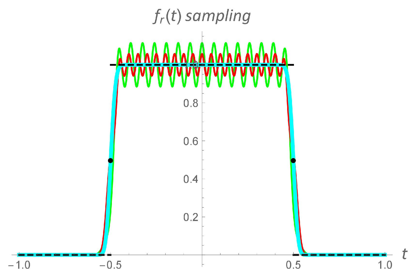
Figure 3.
Fourier transforms of the rectangular and sawtooth functions (dashed black curves) and their approximations (green and magenta curves, respectively).
Figure 3.
Fourier transforms of the rectangular and sawtooth functions (dashed black curves) and their approximations (green and magenta curves, respectively).
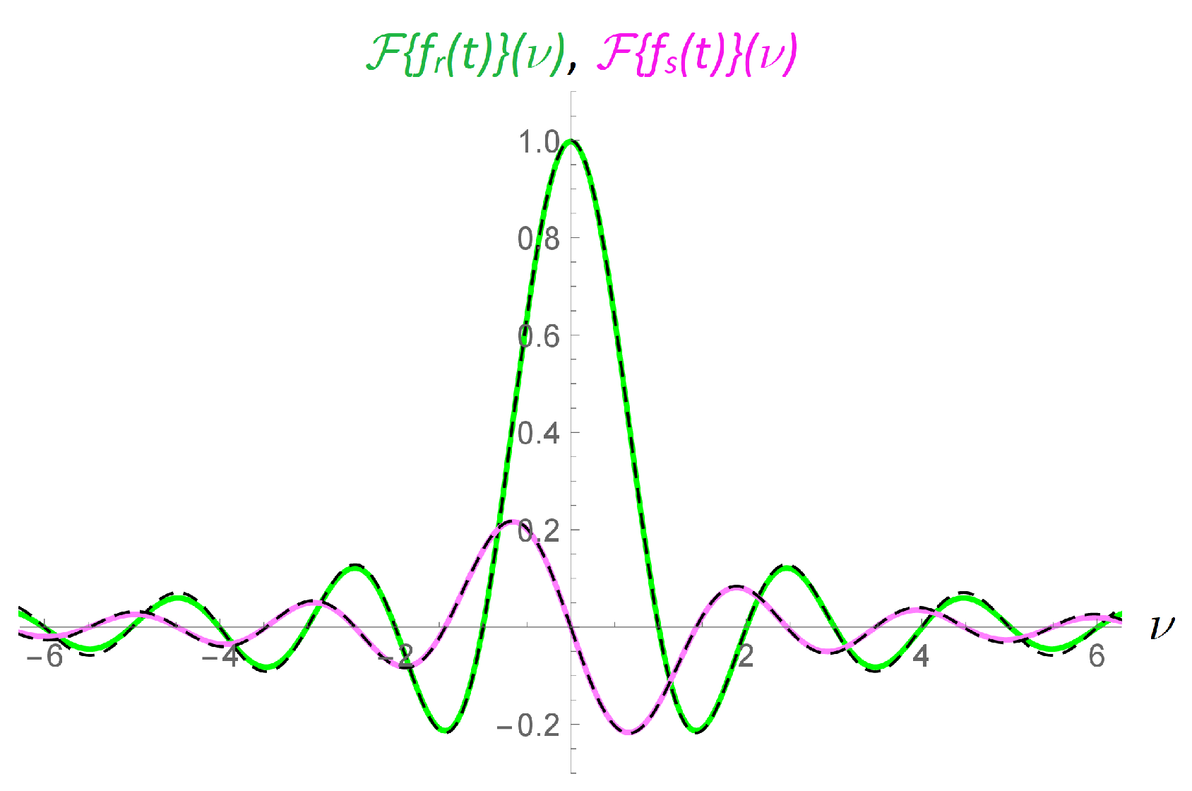
Figure 4.
Absolute differences between equations (35), (36) and their approximations. Blue curve corresponds to equation (35), red curve corresponds to equation (36)).
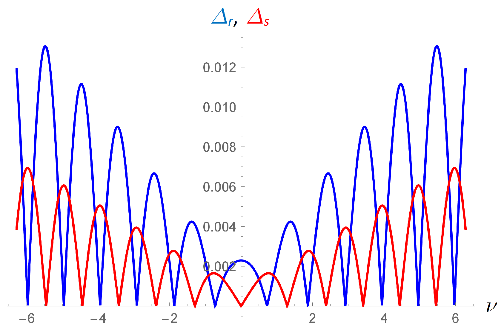
Figure 5.
Equation (37) and its even and odd components (blue, red and green curves, respectively).
Figure 5.
Equation (37) and its even and odd components (blue, red and green curves, respectively).
Disclaimer/Publisher’s Note: The statements, opinions and data contained in all publications are solely those of the individual author(s) and contributor(s) and not of MDPI and/or the editor(s). MDPI and/or the editor(s) disclaim responsibility for any injury to people or property resulting from any ideas, methods, instructions or products referred to in the content. |
© 2025 by the authors. Licensee MDPI, Basel, Switzerland. This article is an open access article distributed under the terms and conditions of the Creative Commons Attribution (CC BY) license (http://creativecommons.org/licenses/by/4.0/).
Copyright: This open access article is published under a Creative Commons CC BY 4.0 license, which permit the free download, distribution, and reuse, provided that the author and preprint are cited in any reuse.


