
Submitted:
07 November 2024
Posted:
11 November 2024
You are already at the latest version
Abstract
Oftentimes in a complex system it is observed that, as a control parameter is varied, there are certain intervals during which the system undergoes dramatic change. Especially in biology, these signatures of criticality are thought to be connected with efficient computation and information processing. Guided by the classical theory of Rate-Distortion (RD) from information theory, we propose a measure for detecting and characterizing such phenomena from data. When applied to RD problems, the measure correctly identifies exact critical trade-off parameters emerging from the theory and allows for the discovery of new conjectures in the field. Other application domains include efficient sensory coding, machine learning generalization, and natural language. Our findings give support to the hypothesis that critical behavior is a signature of optimal processing.
Keywords:
Rate-Distortion
; Optimal Coding
; Criticality
; Phase Transistion
; Kullback-Leibler Divergence
; Generalization
1. Introduction
Criticality has been a hallmark of many fundamental processes in nature. For instance, in classical work, Landau [1] and others [2] investigated critical phase transitions between discrete states of matter. More generally, this concept has been used to describe a complex system that is in sharp transition between two different regimes of behavior as one varies a control parameter. Often, a critical point borders ordered and disordered behavior, such as what occurs in the classical 2D Lenz-Ising spin model of statistical physics at special temperatures [3]. For instance, if the system is too hot then usually disorder prevails; while too cold, and it freezes into a low entropy configuration. The tipping points between such regimes have been the subject of much study in science.
In the recent literature, the notion of criticality [4,5,6] has grown to encompass a computational element [7,8], with an emphasis on how to apply it to understand information processing in natural dynamical systems such as organisms [9,10]. In these applications, it is frequently argued that optimal properties for computation emerge [11,12,13,14,15,16,17] when systems are critically poised at some special set of control parameters. Of particular excitement is how criticality can help neuroscientists understand the brain, and also where such signatures have been observed [18,19,20,21,22,23,24,25,26]. Another exciting area where criticality may be present is in large neural networks which seem to generalize to certain problems at critical scales, training epochs, or dataset sizes [27,28].
Here, we leverage concepts from Rate-Distortion (RD) theory [29,30] to give insight into how normative principles governing a system [31], such as efficient coding [32,33], can lead to critical behavior. Consider a system A that evolves its internal steady-state dynamics through changes in a continuous control parameter t. The equilibrium behavior of A at t is modeled as a conditional distribution , which defines the probability that any given input x results in system state y. We say that A exhibits a critical phase transition about a special value of the control variable if changes dramatically near this parameter setting.
To quantify the change at a given t, we average over inputs x the Kullback-Leibler divergence () between distributions and , with small. We call this a divergence rate for the evolution of the system’s behavior along control parameter t. Given a sample of parameters t, we determine the significant peaks in the divergence rate, which we identify as critical control settings for the system. As we shall see in several examples, local maxima in the divergence rate seem to coincide with locations of phase transitions in a system. Intruigingly, this measure can uncover higher-dimensional manifolds of criticality (Figure 3). This is the equivalent of finding the local maxima in the rate of change in evolving information-theoretic measures [34].
In the language of RD theory, these stochastic Input/Output systems are called codebooks, and they determine – via a rate parameter – a minimal communication rate R for encoding the state x as y given a desired average distortion D. More specifically, the control parameter indexes a pair on the RD function, which separates possible from impossible encodings by a continuous curve in the positive orthant (see Figures 5 and 6).
For example, any lossy compression of a signal class has a particular rate and reconstruction error, which must necessarily lie on or above this curve. Intriguingly, the RD function contains a discrete set of special points that correspond to critical control parameters and codebooks where some states y disappear or reappear in a coding. Intuitively, these are the behavioral phase transitions that must occur when traversing the RD curve from zero to maximal distortion.
In biology, the system A could be an organism that lossily encodes a signal through a channel bottleneck. For example, the retina communicates via the optic nerve to cortex, which is argued to be a several-fold compression of information capture from raw visual input [31]. We may also zoom out in scale to consider collections of organisms. In this setting, the theory of punctuated equilibrium in evolution [35] proposes that species are stable (in equilibrium) until some outside force requires them to change, during which species adapted quickly (punctuation). Here, the control parameter might correspond to some environmental variable in the habitat of the species, and sharp phase transitions [36,37] could emerge from some underlying normative dynamics [38,39,40,41,42].
We first validate our approach on classical RD problems with a number of states n small enough for comparison to mathematically exact calculations. We demonstrate that the critical arising from theory match those that correspond to significant peaks in divergence rate. We also discover in a large-scale numerical experiment that there is an explicit relationship between counts of these critical control parameters and the number of Input/Output states. Namely, under mild assumptions, we conjecture that there are critical , corresponding to critical codebooks and critical pairs , for an RD function on n states (Conjecture 1). As another application, we show how experiments with our measure shed light on the Weak Universality Conjecture [43], which has implications for efficient systems in engineering and in nature.
We next explore several applications to more practical domains. In image processing, for instance, it is commonly desired to encode a picture with a small number of bits that nonetheless represents it faithfully enough for further computation down a channel. In human retina, this is thought to be accomplished by the firing patterns of ON and OFF ganglion neurons, which represent intensity values above or below a local mean, respectively. Using a standard database of natural images [44], we compute the RD function for ON/OFF encodings of small patches and study the structure of its critical . We find that our measure uncovers several significant phase transitions for encoding these natural signals. Interestingly, the number of such critical points on the RD function seems to be significantly smaller than that predicted for a generic RD problem. This finding suggests that natural images define a special class of distributions [45] that might be exploited by visual sensory systems for efficient coding [46].
In machine learning, a common problem is to adapt model parameters for achieving optimal performance on a task. Clustering noisy data is one such challenge, and information theory provides tools for studying its solution [33,47]. We find that critical RD codebooks uncovered by divergence rate can reveal original cluster centers and their count. Another challenge is to store a large collection of patterns in a denoising autoencoder. We examine a specific example of robustly storing an exponential number of memories [48,49] in a Hopfield network [50] given only a small fraction of patterns as training input. We show that as the number of training samples increases, the divergence rate detects critical changes in dynamics, which allow the network to increase performance until generalizing to the full set of desired memories (graph cliques). Thus, we believe that the method of finding criticality described in this paper can be applied to understanding phase transitions in machine learning algorithms. For example, of particular interest is when large language models begin to be able to give the correct answers to certain types of questions [51]. This represents a type of generalization criticality in the space of model parameters.
As a final application, we study critical phenomena in writing. It has been pointed out that phase transitions arise in the geometry of language and knowledge [52,53,54,55,56,57]. We study agriculture during the 1800s in the United States using journal articles and uncover conceptual phase transitions across certain years. In particular, we find that an important shift in written expression occurs during the year 1840. Upon closer examination of the data, there were indeed significant language changes coinciding with the influences of war, religion, and commerce that were occurring at the time.
The outline of this paper is as follows. We give the requisite background for defining divergence rate in Section 2. Next, we explain in Section 3 findings from applying our measure to various domains such as RD theory, sensory coding, machine learning, and language. We close with a discussion in Section 5 and a conclusion in Section 6.
2. Background
We first define a measure of conditional distribution change over an independent control variable, which we call a divergence rate. As the control parameter varies, peaks in this divergence rate can be used to predict critical phase transitions in a system’s behavior. Our methodology is inspired by the work of [54], who used the same measure to compute surprise in a sequence of successive debates of the French Revolution, and hence which topics tended to gain traction. We also give a brief background on rate-distortion theory, which provides a powerful class of examples to validate our approach and its utility as a tool for discovering new results in the field (e.g. Conjecture 1).
2.1. Definition of Measure
Let X be a set of data points with underlying distribution ; that is, the probability of is given by . Also, suppose for real parameters t and each , there are conditional distributions specifying the probability of an output y given input x. The variable t could be a rate-distortion parameter in RD theory, the size of a training dataset, the number of epochs for estimating a model, or simply time. In this work, we restrict our attention to discrete distributions so that X is a finite set.
Definition 1
(Divergence rate).
The following nonegative quantity measures how much a system changes behavior from t to :
The quantity is the Kullback-Leibler divergence of two distributions u and v, although other such functions could be used. The divergence rate is a simple proxy for the rate of change of the system’s behavior. In particular, to detect critical t, we find local maxima in across a range of values of the parameter t.
The following lemma validates the intuition that the divergence rate measures phase transitions.
Lemma 1.
Suppose that for any and that is differentiable at t. Then, the divergence rate limits to zero as goes to zero.
Proof.
Set . Consider the quantity with small for a fixed x, which looks like:
Since , we have , so that the limit of as goes to zero is indeed zero. □
On the other hand, it is easy to verify by its definition that the divergence rate is infinite for any such for all , but for which there is some state y with .
2.2. Determining Critical Control Parameters
To locate critical control parameters of an evolving system , we find all significant local maxima produced by the measure. In practice, numerical imprecision or the presence of noise results in a divergence rate that has several local maxima which likely do not represent critical changes in system behavior. To filter out such false positives, we first normalize the set of divergence rates over samples by subtracting the mean value and then dividing by the standard deviation. This allows us to filter out peaks that are not significant (for example, peaks for some ). From here on, divergence rate will refer to this normalized divergence rate.
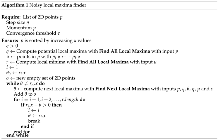
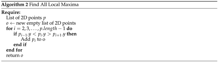
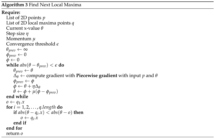
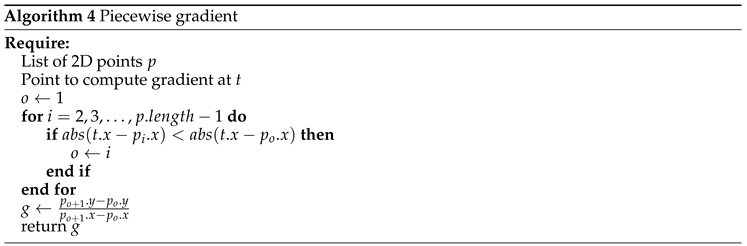
In practice, the divergence rate is potentially non-concave and since t is sampled, we are left with finding peaks in a piecewise linear function. To this end, we utilize a discrete version of the Nesterov momentum algorithm [58] to find significant peaks. We find that the approach is fairly insensitive to hyperparameters when implemented. We provide explicit details of this method and its pseudocode in Section 4.
2.3. Rate-Distortion Theory
Rate-distortion (RD) theory [59] Chapter 10 has frequently been used to analyze and develop lossy compression methods [60] for images [61], video [62], and even memory devices [63]. It also offers some perspective on how biological organisms organize themselves based on their perceptions of the world around them [64]. For example, rate-distortion theory has been used to understand fidelity-efficiency tradeoffs in sensory decision-making [42] and has also been useful in understanding relationships between perception and memory [65]. And at a molecular level, it has been used to study the communication channels and coding properties of proteins [39,66].
Suppose that we have a system with n states and an input probability distribution defined on X. We seek a deterministic coding of x to y, with the overall error arising from this coding determined by a distortion function , which expresses the cost in setting x to y (typically, we assume for all x).
Remarkably, provided only with q and d, the Blahut-Arimoto algorithm [67,68] produces the convex curve of minimal rate over all deterministic codings having a fixed level of average distortion D. For example, when , so that error is not allowed in a coding, the optimal rate is the Shannon entropy of the input distribution q. In general, when , the minimal rate achievable for a coding with average distortion D is less than and is determined by a unique point on RD curve. This is intuitive as a sacrifice of some error in coding should yield a dividend in a better possible rate.
Although the RD curve determines a theoretical boundary between possible and impossible deterministic coding schemes, the curve itself is determined via an optimization over stochastic codings, which do not directly lend themselves to practical deterministic implementations. Nonetheless, computing the RD curve is still useful for understanding the complexity of a given problem and benchmarking. See Figures 5 and 6 for examples of RD curves in various settings.
Mathematically, the RD curve is parameterized by a real number which indexes an optimal stochastic coding of x to y as a codebook or matrix of conditionals (so that ). The average distortion is given by . We also set to be the corresponding distribution for a given output y.
It is classical, using Lagrange multipliers, that points on the RD curve arise from solutions to a set of equations in the codebooks and output distributions. For expositional simplicity in the following, we drop in subscripts and set . We also identify and with and , respectively. The governing equations for the RD curve are then given by the following.
Definition 2.
The Blahut-Arimoto (BA) equations for the RD curve are:
When the numbers are nonnegative integers, solutions to the BA equations form a real algebraic variety, which allows them to be computed symbolically using methods of computational algebra [69].
Example 1
(Two states). When , the three equations translate to these for and :
More generally, set W to be the matrix defined by . (Note that W is invertible near .) Then, equations (1) can be combined into one, as follows:
Here, ⊙ is the point-wise (Hadamard) product of two vectors, is the element-wise ratio of the vectors u and v, and is the transpose of W. Although somewhat surprising given its form, the right-hand side of (3) is indeed in the simplex.
Interestingly, when the BA equations are written in this form, we can identify the RD curve as a fixed-point using Browder’s fixed point theorem [70,71]. We summarize this finding with the following useful characterization.
Proposition 1.
The RD curve is given by the following equivalent objects.
- The minimization of the RD objective function.
- Browder’s fixed-point for the function on the right-hand side of (3).
- Solutions to the BA equations.
Proof.
The equivalence of the first and third statement is classical theory. For the equivalence of the second and the third, consider the map from an interval cross the simplex to the simplex given by . By Browder’s fixed-point theorem, this has a fixed-point given by a curve satisfying , which is equation (3). □
When some of the indeterminates become zero at some , then the BA equations still makes sense, we simply end up with fewer variables. Such equations involving inverses of linear forms also appear in work on the entropic discriminant [72] in algebraic geometry and maximum entropy graph distributions [73].
When is large (w near 0), optimal codebooks are close to the identity, corresponding to average distortion near zero. In this case, it can be shown directly using equations (3) that there is an explicit solution [30]. Set to be the all-ones vector.
Lemma 2.
The exact solution for small w (large β) of the RD function is given by:
Proof.
When is very large, all are nonzero. In this case, we may cancel p on both sides of equation (3) to give:
The lemma now follows by multiplying both sides of this last equation by . □
It turns out that the rate-distortion curve has critical points on it where dramatic shifts in codebooks occur, an observation that was one of our inspirations. For the purposes of this work, these critical are defined when some goes from positive to zero (or visa-versa) as varies.1 Note that the third equation in (1) implies this is when also has such a change. Given this definition, Lemma 1 shows that divergence rate characterizes these critical points.
The first critical can be determined using Lemma 2 as follows.
Corollary 1.
The first critical on the RD curve going from to is the first value of β that makes some entry of the vector in equation (4) equal to zero.
Proof.
In the next section, we shall continue with our two state Example 1 above and compare this theoretical calculation from Corollary 1 to the first critical found by our criticality measure (see Figure 1).
3. Applications
We present applications of finding peaks (Section 2.2) in the divergence rate (Definition 1) to the discovery of phase transitions in various domains such as rate-distortion theory, natural signal modeling, machine learning, and language.
3.1. Rate-Distortion Theory
Recall that given a distribution q and a distortion function d, the rate-distortion curve characterizes the minimal rate of a coding given a fixed average distortion. A point on the curve is specified by a parameter and is determined by an underlying codebook . In particular, the setup for RD theory can be seen as a direct application of our general framework with the control parameter .
In the following subsections, we shall validate our approach to finding critical phase transitions by comparing our peak finder estimates of critical with those afforded by RD theory. In cases where the number of states is small, such as and , we can compute explicit solutions to the RD equations (1) and compare them with those estimated by our divergence rate approach (see Figure 1, Figure 2, Figure 3).
After demonstrating that peaks in divergence rate agree with theory in these cases, we next turn our attention to exploring what our criticality tool can uncover theory-wise for the discipline. In particular, our experiments suggest new results for RD theory, such as that for a random RD problem, the number of critical on n states goes as (Conjecture 1). We also use our framework to help shed light on a universality conjecture [43] inspired by tradeoffs in sensory coding for biology (Conjecture 2).
3.1.1. Exact RD on Two States
The case of states with varying distortion is already interesting. Consider a source distribution and distortion matrix for fixed given by:
In this case, using Lemma 2, one can explicitly solve the equations for the output distributions before the first critical point in terms of (recall, ):
From Corollary 1, the first critical is determined when one of these expressions becomes zero. One can check that for , first has a zero value for some critical . At this value, is automatically determined to be . For , on the other hand, it is that becomes zero.
We consider the case , as the other is similar. Our main tool is the generalized version of Descartes’ Rule of Signs [74,75]. This rule says that an expression in a positive indeterminate w, such as from above, has a number of positive real zeroes bounded above by the number s of sign changes of its coefficients. Moreover, the true number of positive zeroes can only be s, , …, or .
In our particular setting, we have so that there can only be two or no positive zeroes. As is a zero, it follows that there is some other positive number making this expression zero. It follows that our first critical point is . In particular, when , we have:
Given these explicit calculations from the theory in hand, we would like to compare them with critical parameters determined from significant peaks in the divergence rate.
We summarize our findings in Figure 1. To produce the "measured" points in this plot, we vary the distortion measure using the parameter a, compute codebooks parameterized by with the BA algorithm, and then find critical values of at which the divergence rate peaks. At all values of , the critical value of w found by the noisy peak-finder matches the corresponding exact value from the theory (the "algebraic" line). Note that near , the critical approaches zero but is not defined there. Also from the plot, one can guess that approaches (resp. infinity) as a goes to infinity (resp. zero). This can also be verified directly from the theoretical calculations above.
3.1.2. Exact RD on Three States
We now consider a slightly more complicated example from Berger [76] with states. In this case, we assume a varying source for a parameter , but we fix a distortion matrix:
Again using Lemma 2, we find that for large , the output distributions on the RD curve are given by:
For example, when , this becomes:
In this special case, one can check that the first critical occurs when becomes zero; that is, when:
More generally, one can check that as long as , a critical is determined from the formula:
In Figure 2, we plot for three different settings of , the values of the output distribution for the second state as a function of , computed from the general solution (6). On the same plot, we place two circles on the x-axis where we find representing peaks in the divergence rate in the case of . Notice they are located where the output probability of state two goes to zero or emerges from zero.
Figure 3 is obtained by plotting the divergence rate as a heatmap against u and . The peak of the bottom convex shape corresponds to the value of where a discontinuity appears in the number of critical given a fixed u. Also shown in Figure 3 is a theoretically determined part of this curve, which matches precisely the estimated lower-right piece determined only using the divergence rate.
3.1.3. Criticality for Generic RD Theory
With these examples as evidence that the empirical divergence rate is able to detect critical for RD theory, we explore its potential implications for the general case as we increase the number of states n.
We next consider random RD problems on n states in which the probabilities for q are chosen independently from a uniform distribution in the interval (and then normalized to sum to one) and the distortion matrices are chosen to have diagonal zero and other entries drawn independently and uniformly in the interval . (Our experiments appear to be insensitive to the particular underlying distributions used to make q and d.)
In Figure 4, we vary n and plot the number of significant peaks in divergence rate for these random RD problems, averaged over 10 trials. The divergence rate is imperfect and thus there are error bars. The accuracy of the divergence rate depends highly on whether the range of is adequately densely-sampled and that the range of samples includes all critical . It should be noted that this method of finding critical points is an estimate and therefore may indicate large changes in the codebooks where there is no theoretical critical point.
In particular, the numerical results shown in Figure 4 suggest the following new conjecture in the field of RD theory.
Conjecture 1.
Generically, there are critical along the rate-distortion curve as a function of the number of states n.
Here, the word "generic" is used in the sense that an RD problem with data distribution q and distortion matrix d chosen at random will have this number of critical points. More precisely, if and are indeterminates (set one of the to be 1 minus the sum of the others), then outside of a measure zero set in , the conjecture holds.
3.1.4. Weak Universality
Consider the case where all n states have the same probability and two distortion matrices , have entries drawn from the same distribution, say uniform in . Then a conjecture in RD theory, called Weak Universality, says that the RD curves for and lie on top of each other for large n.
Conjecture 2
(Weak Universality [43]). Distortion matrices with entries drawn i.i.d from a fixed distribution ϕ define rate-distortion curves that are (universal) functions of ϕ in the limit of large numbers of states.
To illustrate weak universality in Figure 5, we took two randomly drawn distortion matrices and and plotted their RD curves, computed using the BA algorithm. We then plotted the critical points found from determining peaks in divergence rate on each of the two RD curves. As predicted by Conjecture 2, the RD curves are close. However, notice that the two sets of critical points do not align with each other.
This experiment suggests that we can rule out a line of attack for proving Weak Universality that attempts to show critical points on the RD curve also coincide with each other. In particular, this stronger form of the conjecture is likely not true.
3.2. Natural Signals
Discrete ON/OFF encodings of image patches have been shown to contain much perceptual information [77], and Hopfield Networks trained to store these binary vectors can be used for high quality lossy compression of natural images [78,79].
It was also observed in [80] that these ON/OFF distributions of natural patches exhibited critical at a few special points and codebooks along the RD curve. Applying our noisy peak finder to the divergence rate on the codebooks at rate parameters , we are able to discover all the critical codebooks that were previously found by hand, as well as four more which have deviations in microstructure. We remark that it is also possible that some of these extra critical codebooks found may have arisen from imperfections in the tuning of the peak finder.
To obtain Figure 6, two-by-two pixel patches x are ternarized by first normalizing the pixel values within each patch to have variance one, and then each normalized value v is mapped to a ternary value b via the following rule:
We use as source q the probability distribution over this ternary representation of patches, and the Hamming distance between two binary vectors specifies the distortion matrix. Codebooks along the RD curve are then used as conditional distributions and peaks in the divergence rate are plotted as the 9 blue circles.
In Figure 7, we display the codebooks that arose from the critical found using the divergence rate. These codebooks correspond to the lettered points in Figure 6.
It is interesting to note that there are an order of magnitude fewer critical codebooks estimated than would be expected by Conjecture 1. This suggests that this set of natural signals does not represent a random or generic RD problem, indicating extra structure in the signal class.
3.3. Machine Learning
We consider a warm up problem on 18 states to test the divergence rate on the problem of clustering. The data contains three disjoint groups, each with six states, that have low intra-cluster distortion but high inter-class distortion.
We apply the noisy peak finder to the divergence rate of codebooks parameterizing the RD curve for this setup, and we plot a few of the interesting critical codebooks in Figure 8. We notice that critical codebooks code for when the cluster centers are found, and when the code progressively breaks away towards the identity codebook.
Our next machine learning example comes from the theory of auto-encoding with Hopfield networks. First, we determine networks to store cliques as fixed-point attractors (memories) using Minimum Energy Flow (MEF) learning, as in [48,49]. Then, we look for peaks in divergence rate as networks are trained with different numbers of samples s. Our hypothesis is that as s is varied, there should be some critical s where the nature of network dynamics changes drastically.
For the clique example in Figure 9, the possible data consist of binary vectors representing absence or presence of an edge in a graph of size 16, with each sample being a clique of size 8.
By randomly sampling a different set of training data for each trial, we obtain a codebook for each number of training samples as the deterministic map on binary vectors given by the dynamics of the Hopfield network. Specifically, the codebook is the 0/1-matrix of the output of the dynamics determined by the association of the sth network; that is, each map forms a conditional matrix entry that is if the network dynamics takes state x to y, and zero, otherwise, where is the total number of cliques. We use one output state state to code for all non-cliques, leading to in the denominator.
We then plot the accuracy (proportion of cliques correctly stored by the network) in blue and the normalized divergence rate in orange against s. We averaged over 10 trials in the experiment.
A significant peak in the divergence rate as a function of s can be observed in Figure 9. This suggests that is a critical sample count for auto-encoding in Hopfield networks trained using MEF. Note that this peak appears to occur when half of the test data is accurately coded.
3.4. Language
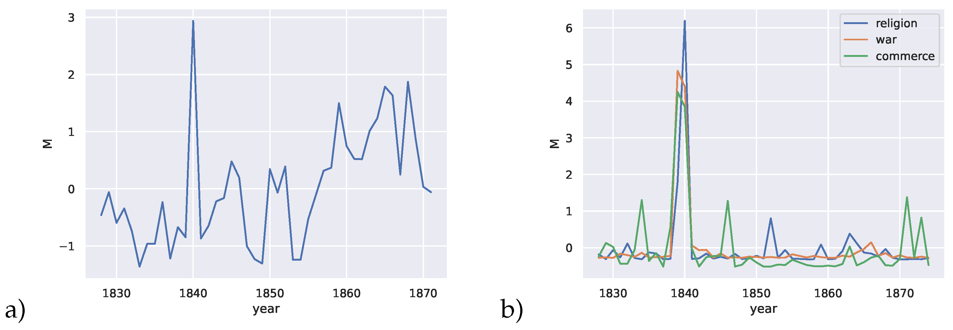
In [55], the possibility of punctuated equilibrium and criticality in language evolution was studied using a similar approach based on the divergence rate. Naively using the divergence rate on raw word frequency distributions over time, we can also obtain a measure of language change over time. In this case, the divergence rate is over a single condition (fixed topic). We show that peaks are also observed in this measure of a language dataset; see Figure 10a, which indicates that critical changes are not only common, but a natural part of the way humans solve problems in communication.
For the language example, the codebook is conditioned on a single state, which is the topic of the dataset; namely, agriculture in America. This means we only consider the distribution of words of one topic over time as the independent variable t. The divergence rate is thus applied over a single state in the language concept space.
To discover what the underlying cause of this large change could be, we clustered the words in the corpus using Word2Vec [82] and find several interesting clusters. We then chose semantically similar words from those clusters, which represent concepts in war, religion and commerce. Again, by conditioning on words from these subtopics, we use the divergence rate to obtain the changes in the probability distributions of these clusters individually in Figure 10b. We notice that peaks occur exactly in the year of the most significant peak in Figure 10a.
Investigating possible reasons why this might be the case, we looked to the history of agriculture in the United States of America. In [83], Frolik mentioned that many innovations and technologies came to bear on the American agriculture industry (such as the cast iron plow, manufacturing of drills for sowing seeds, and horse-powered machines for harvesting grain) around the years leading up to and including the 1840s, which led to a booming agricultural industry. This possibly accounts for the peak in usage of words related to commerce.
4. Methods
The measure is the sum of the distance over between probability distributions f conditioned on x at different points t and . It tracks the change in f over t. In our experiments, we used the Kullback-Leibler (KL) divergence for D.
The value of t here could be replaced by some independent variable, such as (in the case of the RD curve), size of training dataset, number of epochs (for training a model), or time. The codebook of a model f (for a discrete state space) is a distribution conditioned on each input state. For a set of models with random initializations, we normalize the distribution of the maps with respect to the inputs over all the maps. The measure over t is then obtained by taking the distance between codebooks between pairs of consecutive codebooks. Critical phase transitions are then where peaks occur along this 1-dimensional signal.
The measure is potentially non-concave and the variable t is usually sampled at discrete intervals, thus producing a piecewise linear function. Thus, to detect local maxima in the measure which represent points in t where the measure changes significantly (a critical point in t), we need a noisy peak finder, as there may be spurious local maxima which do not correspond to any critical change in behavior. To this end, we develop a discrete version of Nesterov momentum algorithm [58] in Algorithm 1.
Given a distortion measure (non-negative matrix describing costs of encoding an input state with an output state), the rate-distortion curve describes the minimum amount of information required to encode a given distribution of symbols at a level of distortion specified by the gain parameter . There is a corresponding codebook at any , which describes a distribution over all symbols X for each symbol x with which to optimally code for x. This allows us to directly use the measure, using as the independent variable t.
For the simple two-state rate-distortion example in Figure 1, we vary the distortion measure using a parameter a and find the critical value of at which the measure peaks. At all values of a, the critical value of found by the noisy peak-finder matches the analytic critical value of . Note that there is no analytic critical value of at , and thus there is a gap in the plot.
For the three-state case proposed by Berger in Figure 2 and Figure 3, the distortion matrix is held constant and we vary the probability distribution q. As an example, Figure 2 shows the marginal probability of state 2 at , and the points show where the peak-finder detects a critical change, which are visually exactly where the marginal probability goes to or emerges from 0. Figure 3 was made by plotting the measure as a heatmap against u, .
To arrive at Figure 4, we generate a random distortion matrix for a uniform distribution on k states for each trial. We vary k and plot the number of critical against k for the RD curve on this setup. We perform 10 trials to obtain this plot.
To illustrate weak universality in Figure 5, we took two probability vectors P1 and P2 drawn from the same distribution with corresponding distortion matrices D1 and D2 also drawn from the same distribution. We then plotted the critical points found by the measure on the RD curve.
To test this measure on the coding of clusters, we consider a 18-state distribution, with disjoint groups of six states that have low intra-cluster distortion, but high inter-class distortion. We then apply the noisy peak finder to the measure on the RD curve for this setup and plot some of the interesting critical codebooks in Figure 8 and the corresponding critical points on the RD curve and measure in Figure 8.
For the clique example in Figure 9, the data is binary vectors representing absence or presence of an edge in a graph, with each sample being a clique of size , where v is the number of nodes in the graph, taken to be 8 in our experiment. The distortion matrix is computed using Hamming distance. By randomly sampling a different set of training data for each trial, we obtain a codebook for each number of training samples by normalizing the . We then plot the accuracy (proportion of cliques correctly stored by the network) in green and the normalized measure in purple against the number of training samples.
In the natural image patch example in Figure 6, the data is a ternarized form of two by two pixel patches. Each pixel is normalized and then represented by two bits. If the normalized value of the pixel is greater than a threshold value , it is represented as , if it is less than , it is represented by , otherwise, it is represented by . Thus in a two by two patch, there are states. Again, the distortion matrix is the Hamming distance between two bit vectors. We obtain codebooks along the RD curve and plot points where critical transitions are found.
For the language example, the codebook is conditioned on a single variable, which is the topic of the dataset; agriculture in America. This means we only consider the distribution of words of one topic over time as the independent variable t. The measure is thus over a single state in the language concept space.
5. Discussion
In this section, we discuss implications of our criticality measure. Our experiments show that criticality in system behavior appears to be relatively common, as predicted by RD theory. In this paper, we have shown that optimization procedures can also lead to critical transitions in function behavior and that in natural processes such as language evolution, such critical changes can also occur. It could be that these processes find encodings that are close to rate-optimal, as there may be a significant discontinuous change in the rate of change of encoding cost with respect to encoding error at these points. This means that approaching this point from a higher distortion would suddenly incur a higher cost of encoding for the same distortion at this point, and approaching it from a lower distortion would result in a sudden drop in encoding fidelity for the same reduction in encoding cost.
This analysis however, only accounts for the critical points on the RD curve. The critical points of a process would depend on the details of the process itself, and we can only expect the critical points to line up with the ones on the RD curve if the process is efficient enough to follow the RD curve near its critical points. It is possible to detect these discontinuities in , though measuring it would require far more samples.
Another point that can be made is that criticality does not necessarily manifest as points, but manifolds. In Figure 3, a 1-dimensional critical manifold is observed in u. This is akin to how the boiling point of a substance is a function of pressure and temperature. Further work could involve studying the behavior of these manifolds.
Observing the codebooks at the critical points in order of increasing distortion, we find that the codebook breaks away further from encoding the distribution as the identity function. Further work could be to observe the microstructure of codebooks at the critical points to try to understand which states are chosen to reduce the cost of coding perfectly at each critical point.
There are several direct implications for critical behavior, some of which were outlined by Sims in [84]. One open question is how to apply these ideas to deep learning [85] which minimize a typically squared error loss. An insight is to choose models and normative principles that have critical signatures [65] (working memory). Given that optimal continuous codings are discrete [80,86,87,88], it is not that surprising for criticality to arise from near-optimal solutions to normative principles applied to information processing. Furthermore, it has been observed that generalization beyond overfitting a training dataset, such as that seen in grokking by large language models, is related to the double descent phenomena [28], which has been shown to be dependent on multiple factors [89]. These relationships could be further explored using the method described in this paper, by for example, estimating the of more complex distributions using [90].
Further work would involve continuous distributions which require a different treatment to obtain the RD curves and different probability distribution distance metrics. Other algorithms for mapping discrete spaces could also be analyzed with the techniques developed in this work.
6. Conclusion
Our initial hypothesis was that an information processing system which compresses and reinterprets information into a useful form usually has critical transitions in the way the information is transformed as some control parameter of the system is tweaked. This was confirmed with the use of divergence rate – the measure we developed to track the change in the maps along the control parameter – and a noisy peak finder which helped to identify the critical points. We believe this may provide fertile ground for further research into critical phenomena in other maps such as the behavior of learning algorithms.
Acknowledgments
We thank Sarah Marzen and Lav Varshney for their input on this work.
Conflicts of Interest
The authors declare no conflict of interest.
Abbreviations
The following abbreviations are used in this manuscript:
| RD | Rate-Distortion |
| Kullback-Leibler Divergence | |
| MEF | Minimum Energy Flow |
References
- Landau, L. The Theory of Phase Transitions. Nature 1936, 138, 840–841. [Google Scholar] [CrossRef]
- Anisimov, M.A. Letter to the Editor: Fifty Years of Breakthrough Discoveries in Fluid Criticality. International Journal of Thermophysics 2011, 32, 2001–2009. [Google Scholar] [CrossRef]
- Peierls, R. On Ising’s model of ferromagnetism. Mathematical Proceedings of the Cambridge Philosophical Society 1936, 32, 477–481. [Google Scholar] [CrossRef]
- Bak, P.; Chen, K. The physics of fractals. Physica D: Nonlinear Phenomena 1989, 38, 5–12. [Google Scholar] [CrossRef]
- Paczuski, M.; Maslov, S.; Bak, P. Avalanche dynamics in evolution, growth, and depinning models. Physical Review E 1996, 53, 414–443. [Google Scholar] [CrossRef]
- Watkins, N.W.; Pruessner, G.; Chapman, S.C.; Crosby, N.B.; Jensen, H.J. 25 years of self-organized criticality: concepts and controversies. Space Science Reviews 2016, 198, 3–44. [Google Scholar] [CrossRef]
- Langton, C.G. Computation at the edge of chaos: Phase transitions and emergent computation. Physica D: Nonlinear Phenomena 1990, 42, 12–37. [Google Scholar] [CrossRef]
- Prokopenko, M. Modelling complex systems and guided self-organisation. Journal & Proceedings of the Royal Society of New South Wales 2017, 150, 104–109. [Google Scholar]
- Mora, T.; Bialek, W. Are Biological Systems Poised at Criticality? Journal of Statistical Physics 2011, 144, 268–302. [Google Scholar] [CrossRef]
- Muñoz, M.A. Colloquium : Criticality and dynamical scaling in living systems. Reviews of Modern Physics 2018, 90, 031001. [Google Scholar] [CrossRef]
- Bertschinger, N.; Natschläger, T. Real-Time Computation at the Edge of Chaos in Recurrent Neural Networks. Neural Computation 2004, 16, 1413–1436. [Google Scholar] [CrossRef] [PubMed]
- Kinouchi, O.; Copelli, M. Optimal dynamical range of excitable networks at criticality. Nature Physics 2006, 2, 348–351. [Google Scholar] [CrossRef]
- Legenstein, R.; Maass, W. Edge of chaos and prediction of computational performance for neural circuit models. Neural Networks 2007, 20, 323–334. [Google Scholar] [CrossRef] [PubMed]
- Boedecker, J.; Obst, O.; Lizier, J.T.; Mayer, N.M.; Asada, M. Information processing in echo state networks at the edge of chaos. Theory in Biosciences 2012, 131, 205–213. [Google Scholar] [CrossRef]
- Hoffmann, H.; Payton, D.W. Optimization by Self-Organized Criticality. Scientific Reports 2018, 8, 2358. [Google Scholar] [CrossRef]
- Wilting, J.; Priesemann, V. Inferring collective dynamical states from widely unobserved systems. Nature Communications 2018, 9, 2325. [Google Scholar] [CrossRef]
- Avramiea, A.E.; Masood, A.; Mansvelder, H.D.; Linkenkaer-Hansen, K. Long-Range Amplitude Coupling Is Optimized for Brain Networks That Function at Criticality. The Journal of Neuroscience 2022, 42, 2221–2233. [Google Scholar] [CrossRef]
- Kelso, J.A. Phase transitions and critical behavior in human bimanual coordination. American Journal of Physiology-Regulatory, Integrative and Comparative Physiology 1984, 246, R1000–R1004. [Google Scholar] [CrossRef]
- Shew, W.L.; Plenz, D. The Functional Benefits of Criticality in the Cortex. The Neuroscientist 2013, 19, 88–100. [Google Scholar] [CrossRef]
- Tkačik, G.; Bialek, W. Information Processing in Living Systems. Annual Review of Condensed Matter Physics 2016, 7, 89–117. [Google Scholar] [CrossRef]
- Erten, E.; Lizier, J.; Piraveenan, M.; Prokopenko, M. Criticality and Information Dynamics in Epidemiological Models. Entropy 2017, 19, 194. [Google Scholar] [CrossRef]
- Cocchi, L.; Gollo, L.L.; Zalesky, A.; Breakspear, M. Criticality in the brain: A synthesis of neurobiology, models and cognition. Progress in Neurobiology 2017, 158, 132–152. [Google Scholar] [CrossRef] [PubMed]
- Zimmern, V. Why Brain Criticality Is Clinically Relevant: A Scoping Review. Frontiers in Neural Circuits 2020, 14, 54. [Google Scholar] [CrossRef] [PubMed]
- Cramer, B.; Stöckel, D.; Kreft, M.; Wibral, M.; Schemmel, J.; Meier, K.; Priesemann, V. Control of criticality and computation in spiking neuromorphic networks with plasticity. Nature Communications 2020, 11, 2853. [Google Scholar] [CrossRef]
- Heiney, K.; Huse Ramstad, O.; Fiskum, V.; Christiansen, N.; Sandvig, A.; Nichele, S.; Sandvig, I. Criticality, Connectivity, and Neural Disorder: A Multifaceted Approach to Neural Computation. Frontiers in Computational Neuroscience 2021, 15, 611183. [Google Scholar] [CrossRef]
- O’Byrne, J.; Jerbi, K. How critical is brain criticality? Trends in Neurosciences 2022, 45, 820–837. [Google Scholar] [CrossRef]
- Power, A.; Burda, Y.; Edwards, H.; Babuschkin, I.; Misra, V. Grokking: Generalization beyond overfitting on small algorithmic datasets. arXiv preprint, arXiv:2201.02177 2022.
- Liu, Z.; Kitouni, O.; Nolte, N.S.; Michaud, E.; Tegmark, M.; Williams, M. Towards understanding grokking: An effective theory of representation learning. Advances in Neural Information Processing Systems 2022, 35, 34651–34663. [Google Scholar]
- Shannon, C.E. Probability of Error for Optimal Codes in a Gaussian Channel. Bell System Technical Journal 1959, 38, 611–656. [Google Scholar] [CrossRef]
- Berger, T. Rate Distortion Theory and Data Compression. In Advances in Source Coding; Springer Vienna: Vienna, 1975; pp. 1–39. [Google Scholar] [CrossRef]
- Sterling, P.; Laughlin, S. Principles of Neural Design; The MIT Press, 2015. [CrossRef]
- Barlow, H.B. Possible Principles Underlying the Transformations of Sensory Messages. In Sensory Communication; Rosenblith, W.A., Ed.; The MIT Press, 1961; pp. 216–234. [CrossRef]
- Rose, K. Deterministic annealing for clustering, compression, classification, regression, and related optimization problems. Proceedings of the IEEE 1998, 86, 2210–2239. [Google Scholar] [CrossRef]
- Wibisono, A.; Jog, V.; Loh, P.L. Information and estimation in Fokker-Planck channels. 2017 IEEE International Symposium on Information Theory (ISIT). IEEE, 2017, pp. 2673–2677.
- Gould, S.J.; Eldredge, N. Punctuated equilibria: an alternative to phyletic gradualism. In Models in paleobiology; Freeman, Cooper, 1972.
- Wallace, R.; Wallace, D. Punctuated Equilibrium in Statistical Models of Generalized Coevolutionary Resilience: How Sudden Ecosystem Transitions Can Entrain Both Phenotype Expression and Darwinian Selection. In Transactions on Computational Systems Biology IX; Istrail, S.; Pevzner, P.; Waterman, M.S.; Priami, C., Eds.; Springer Berlin Heidelberg: Berlin, Heidelberg, 2008; Vol. 5121, pp. 23–85. Series Title: Lecture Notes in Computer Science. [CrossRef]
- King, D.M. Classification of Phase Transition Behavior in a Model of Evolutionary Dynamics. PhD thesis, University of Missouri-St. Louis, 2012.
- Wallace, R. Adaptation, Punctuation and Information: A Rate-Distortion Approach to Non-Cognitive ’Learning Plateaus’ in evolutionary processes. Acta Biotheoretica 2002, 50, 101–116. [Google Scholar] [CrossRef]
- Tlusty, T. A model for the emergence of the genetic code as a transition in a noisy information channel. Journal of Theoretical Biology 2007, 249, 331–342. [Google Scholar] [CrossRef] [PubMed]
- Tlusty, T. A rate-distortion scenario for the emergence and evolution of noisy molecular codes. Physical Review Letters 2008, 100, 048101. [Google Scholar] [CrossRef] [PubMed]
- Liuling Gong. ; Bouaynaya, N.; Schonfeld, D. Information-Theoretic Model of Evolution over Protein Communication Channel. IEEE/ACM Transactions on Computational Biology and Bioinformatics 2011, 8, 143–151. [Google Scholar] [CrossRef] [PubMed]
- Marzen, S.E.; DeDeo, S. The evolution of lossy compression. Journal of The Royal Society Interface 2017, 14, 20170166. [Google Scholar] [CrossRef] [PubMed]
- Marzen, S.; DeDeo, S. Weak universality in sensory tradeoffs. Physical Review E 2016, 94, 060101. [Google Scholar] [CrossRef]
- van der Schaaf, A.; van Hateren, J. Modelling the Power Spectra of Natural Images: Statistics and Information. Vision Research 1996, 36, 2759–2770. [Google Scholar] [CrossRef]
- Ruderman, D.L.; Bialek, W. Statistics of natural images: Scaling in the woods. Physical Review Letters 1994, 73, 814–817. [Google Scholar] [CrossRef]
- Zhaoping, L. Understanding Vision: Theory, Models, and Data, 1 ed.; Oxford University PressOxford, 2014.
- Sugar, C.A.; James, G.M. Finding the Number of Clusters in a Dataset: An Information-Theoretic Approach. Journal of the American Statistical Association 2003, 98, 750–763. [Google Scholar] [CrossRef]
- Hillar, C.J.; Tran, N.M. Robust Exponential Memory in Hopfield Networks. The Journal of Mathematical Neuroscience 2018, 8, 1. [Google Scholar] [CrossRef]
- Hillar, C.; Chan, T.; Taubman, R.; Rolnick, D. Hidden Hypergraphs, Error-Correcting Codes, and Critical Learning in Hopfield Networks. Entropy 2021, 23, 1494. [Google Scholar] [CrossRef]
- Hopfield, J.J. Neural networks and physical systems with emergent collective computational abilities. Proceedings of the National Academy of Sciences 1982, 79, 2554–2558. [Google Scholar] [CrossRef] [PubMed]
- Humayun, A.I.; Balestriero, R.; Baraniuk, R. Deep networks always grok and here is why. arXiv preprint arXiv:2402.15555 2024, arXiv:2402.15555.
- Bowern, C. Punctuated Equilibrium and Language Change. In Encyclopedia of Language & Linguistics; Elsevier, 2006; pp. 286–289. [CrossRef]
- Tadic, B.; Dankulov, M.M.; Melnik, R. The mechanisms of self-organised criticality in social processes of knowledge creation. Physical Review E 2017, 96, 032307. [Google Scholar] [CrossRef] [PubMed]
- Barron, A.T.J.; Huang, J.; Spang, R.L.; DeDeo, S. Individuals, institutions, and innovation in the debates of the French Revolution. Proceedings of the National Academy of Sciences 2018, 115, 4607–4612, Publisher: Proceedings of the National Academy of Sciences. [Google Scholar] [CrossRef] [PubMed]
- Nevalainen, T.; Säily, T.; Vartiainen, T.; Liimatta, A.; Lijffijt, J. History of English as punctuated equilibria? A meta-analysis of the rate of linguistic change in Middle English. Journal of Historical Sociolinguistics 2020, 6. Publisher: De Gruyter Mouton. [Google Scholar] [CrossRef]
- Gupta, R.; Roy, S.; Meel, K.S. Phase Transition Behavior in Knowledge Compilation. In Principles and Practice of Constraint Programming; Simonis, H., Ed.; Springer International Publishing: Cham, 2020; Vol. 12333, pp. 358–374. Series Title: Lecture Notes in Computer Science. [CrossRef]
- Seoane, L.F.; Solé, R. Criticality in Pareto Optimal Grammars? Entropy 2020, 22, 165, Number: 2 Publisher: Multidisciplinary Digital Publishing Institute. [Google Scholar] [CrossRef]
- Nesterov, Y. A method for solving the convex programming problem with convergence rate O(1/k⌃2). Proceedings of the USSR Academy of Sciences 1983, 269, 543–547. [Google Scholar]
- Cover, T.M.; Thomas, J.A. Elements of Information Theory, 2nd ed ed.; Wiley-Interscience: Hoboken, N.J, 2006. OCLC: ocm59879802.
- Davisson, L. Rate Distortion Theory: A Mathematical Basis for Data Compression. IEEE Transactions on Communications 1972, 20, 1202–1202, Conference Name: IEEE Transactions on Communications. [Google Scholar] [CrossRef]
- Fang, H.C.; Huang, C.T.; Chang, Y.W.; Wang, T.C.; Tseng, P.C.; Lian, C.J.; Chen, L.G. 81MS/s JPEG2000 single-chip encoder with rate-distortion optimization. 2004 IEEE International Solid-State Circuits Conference (IEEE Cat. No.04CH37519), 2004, pp. 328–531 Vol.1. ISSN: 0193-6530. [CrossRef]
- Choi, I.; Lee, J.; Jeon, B. Fast Coding Mode Selection With Rate-Distortion Optimization for MPEG-4 Part-10 AVC/H.264. IEEE Transactions on Circuits and Systems for Video Technology 2006, 16, 1557–1561, Conference Name: IEEE Transactions on Circuits and Systems for Video Technology. [Google Scholar] [CrossRef]
- Zarcone, R.V.; Engel, J.H.; Burc Eryilmaz, S.; Wan, W.; Kim, S.; BrightSky, M.; Lam, C.; Lung, H.L.; Olshausen, B.A.; Philip Wong, H.S. Analog Coding in Emerging Memory Systems. Scientific Reports 2020, 10, 6831. [Google Scholar] [CrossRef]
- Sims, C.R. Rate–distortion theory and human perception. Cognition 2016, 152, 181–198. [Google Scholar] [CrossRef]
- Jakob, A.M.; Gershman, S.J. Rate-distortion theory of neural coding and its implications for working memory. preprint, Neuroscience, 2022. [CrossRef]
- Wallace, R. A Rate Distortion approach to protein symmetry. Nature Precedings, 2010; 14. [Google Scholar] [CrossRef]
- Blahut, R. Computation of channel capacity and rate-distortion functions. IEEE Transactions on Information Theory 1972, 18, 460–473, Conference Name: IEEE Transactions on Information Theory. [Google Scholar] [CrossRef]
- Arimoto, S. An algorithm for computing the capacity of arbitrary discrete memoryless channels. IEEE Transactions on Information Theory 1972, 18, 14–20, Conference Name: IEEE Transactions on Information Theory. [Google Scholar] [CrossRef]
- Cox, D.A.; Little, J.; O’shea, D. Using algebraic geometry; Vol. 185, Springer Science & Business Media, 2005.
- Browder, F.E. On continuity of fixed points under deformations of continuous mappings. Summa Brasiliensis Mathematicae 1960, 4, 183–191. [Google Scholar]
- Solan, E.; Solan, O.N. Browder’s theorem through brouwer’s fixed point theorem. The American Mathematical Monthly 2023, 130, 370–374. [Google Scholar] [CrossRef]
- Sanyal, R.; Sturmfels, B.; Vinzant, C. The entropic discriminant. Advances in Mathematics 2013, 244, 678–707. [Google Scholar] [CrossRef]
- Hillar, C.; Wibisono, A. Maximum entropy distributions on graphs, 2013. Publisher: arXiv Version Number: 3. [CrossRef]
- Wang, X. A Simple Proof of Descartes’s Rule of Signs. The American Mathematical Monthly 2004, 111, 525. [Google Scholar] [CrossRef]
- Haukkanen, P.; Tossavainen, T. A generalization of Descartes’ rule of signs and fundamental theorem of algebra. Applied Mathematics and Computation 2011, 218, 1203–1207. [Google Scholar] [CrossRef]
- Berger, T. Rate-Distortion Theory. In Wiley Encyclopedia of Telecommunications; Proakis, J.G., Ed.; John Wiley & Sons, Inc.: Hoboken, NJ, USA, 2003; p. eot142. [CrossRef]
- Hillar, C.; Marzen, S. Revisiting Perceptual Distortion for Natural Images: Mean Discrete Structural Similarity Index. 2017 Data Compression Conference (DCC); IEEE: Snowbird, UT, USA, 2017; pp. 241–249. [CrossRef]
- Hillar, C.; Mehta, R.; Koepsell, K. A Hopfield recurrent neural network trained on natural images performs state-of-the-art image compression. 2014 IEEE International Conference on Image Processing (ICIP); IEEE: Paris, France, 2014; pp. 4092–4096. [Google Scholar] [CrossRef]
- Mehta, R.; Marzen, S.; Hillar, C. Exploring discrete approaches to lossy compression schemes for natural image patches. 2015 23rd European Signal Processing Conference (EUSIPCO); IEEE: Nice, 2015; pp. 2236–2240. [Google Scholar] [CrossRef]
- Hillar, C.J.; Marzen, S.E. Neural network coding of natural images with applications to pure mathematics. In Algebraic and Geometric Methods in Discrete Mathematics; American Mathematical Society, 2017; pp. 189–221.
- Del Papa, B.; Priesemann, V.; Triesch, J. Criticality meets learning: Criticality signatures in a self-organizing recurrent neural network. PLOS ONE 2017, 12, e0178683. [Google Scholar] [CrossRef]
- Mikolov, T. Efficient estimation of word representations in vector space. arXiv preprint arXiv:1301.3781 2013, arXiv:1301.3781 2013, 37813781. [Google Scholar]
- Frolik, E. The History of Agriculture in the United States Beginning With the Seventeenth Century. Transactions of the Nebraska Academy of Sciences and Affiliated Societies 1977. [Google Scholar]
- Jung, J.; Kim, J.H.J.; Matějka, F.; Sims, C.A. Discrete Actions in Information-Constrained Decision Problems. The Review of Economic Studies 2019, 86, 2643–2667. [Google Scholar] [CrossRef]
- Grohs, P.; Klotz, A.; Voigtlaender, F. Phase Transitions in Rate Distortion Theory and Deep Learning. Foundations of Computational Mathematics 2021. [Google Scholar] [CrossRef]
- Smith, J.G. The information capacity of amplitude- and variance-constrained scalar gaussian channels. Information and Control 1971, 18, 203–219. [Google Scholar] [CrossRef]
- Fix, S.L. Rate distortion functions for squared error distortion measures. Annual Allerton Conference on Communication, Control and Computing, 1978, pp. 704–711.
- Rose, K. A mapping approach to rate-distortion computation and analysis. IEEE Transactions on Information Theory 1994, 40, 1939–1952. [Google Scholar] [CrossRef]
- Schaeffer, R.; Khona, M.; Robertson, Z.; Boopathy, A.; Pistunova, K.; Rocks, J.W.; Fiete, I.R.; Koyejo, O. Double descent demystified: Identifying, interpreting & ablating the sources of a deep learning puzzle. arXiv preprint, arXiv:2303.14151 2023.
- Borade, S.; Zheng, L. Euclidean information theory. 2008 IEEE International Zurich Seminar on Communications. IEEE, 2008, pp. 14–17.
| 1 | We remark that in the literature, another equivalent definition is usually used, which is when the derivative of the RD curve has a discontinuity. |
Figure 1.
Critical RD parameters determined mathematically from the theory (algebraic) match up exactly with significant peaks in divergence rate (measured) (Left). Plotting M vs w for three different values of a shows the single peak in the divergence rate M (Right).
Figure 1.
Critical RD parameters determined mathematically from the theory (algebraic) match up exactly with significant peaks in divergence rate (measured) (Left). Plotting M vs w for three different values of a shows the single peak in the divergence rate M (Right).
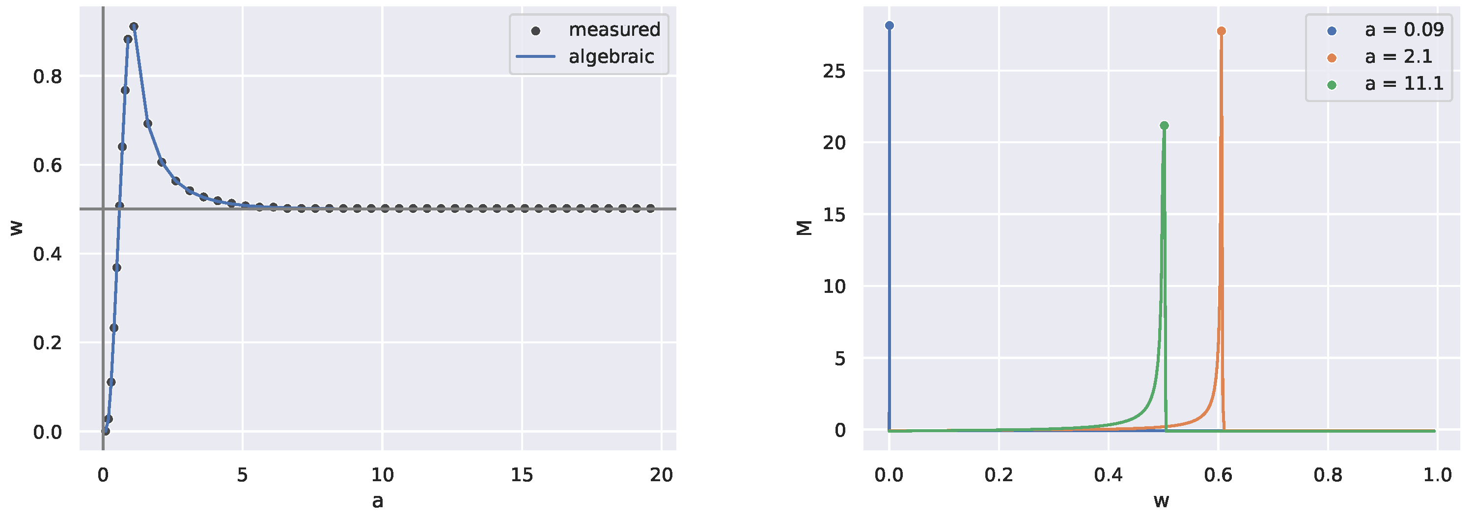
Figure 2.
Consider for a parameter u and a fixed distortion d given by (5). For each , we plot the output probabilities of the second state as a function of , determined by the exact theory. The circles were determined from finding significant peaks in divergence rate at and match the vanishing and re-emergence of state 2.
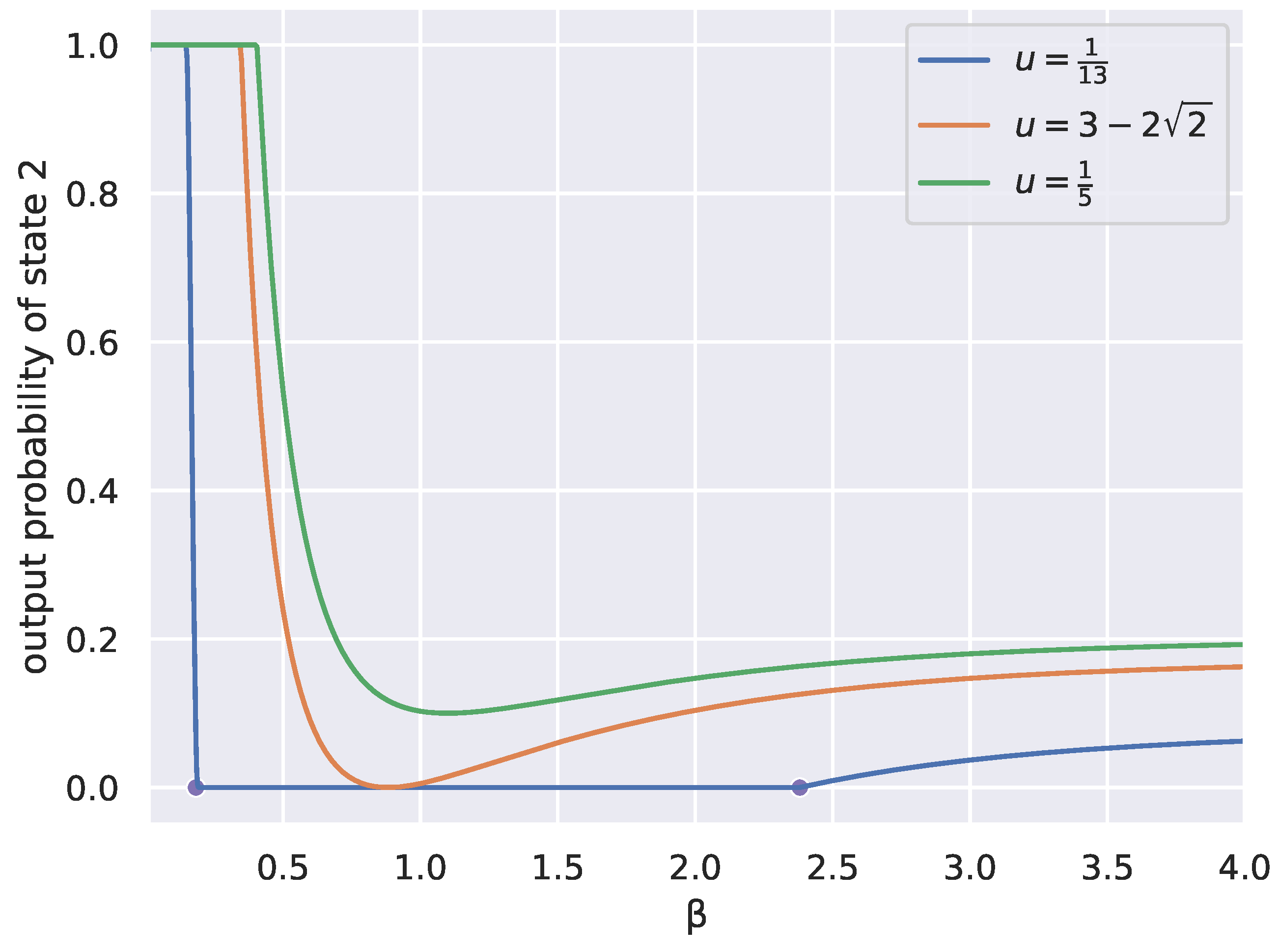
Figure 3.
We plot a heatmap of the divergence rate as a function of u and . We also plot the theoretical calculation matching the lower-right part of the curve in the heatmap in green.
Figure 3.
We plot a heatmap of the divergence rate as a function of u and . We also plot the theoretical calculation matching the lower-right part of the curve in the heatmap in green.
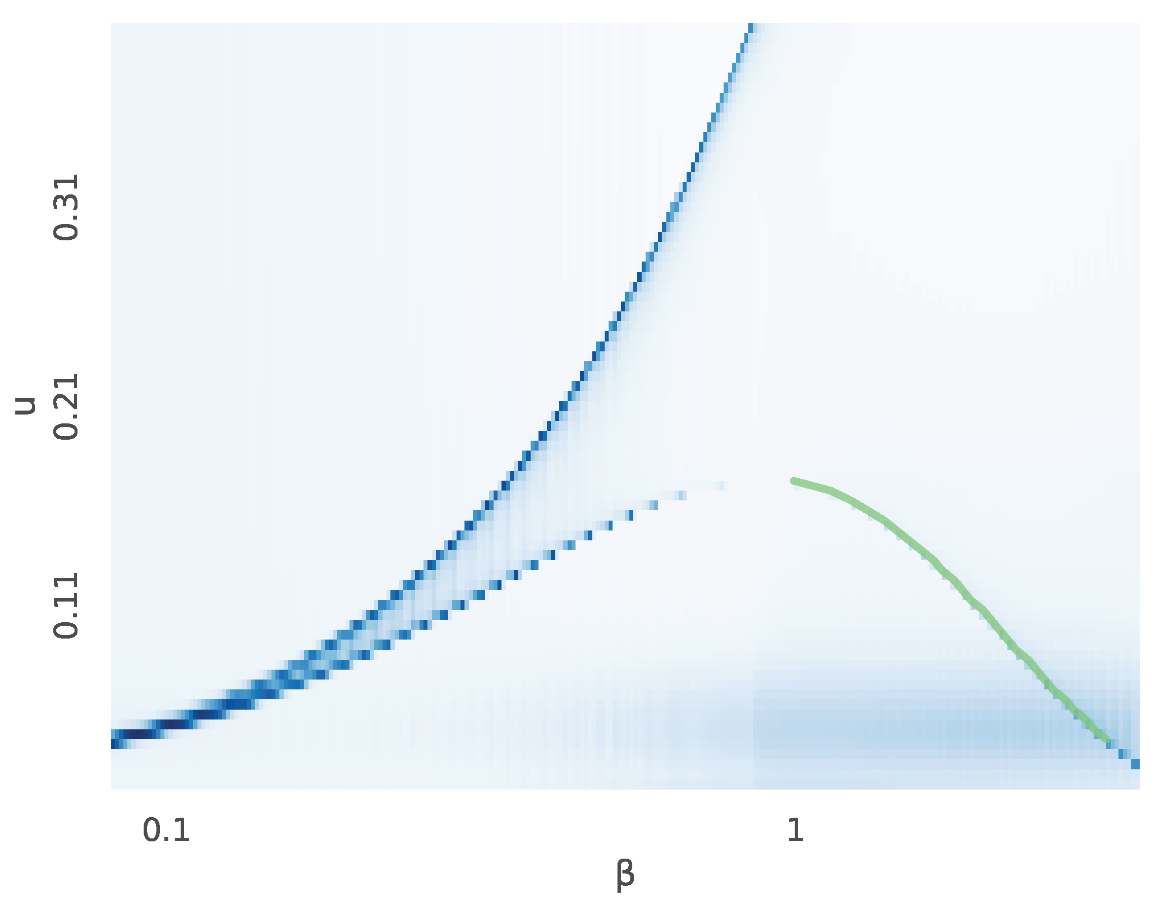
Figure 4.
The number of peaks in the divergence rate across different values of for varying numbers of states n is close to the line .
Figure 4.
The number of peaks in the divergence rate across different values of for varying numbers of states n is close to the line .
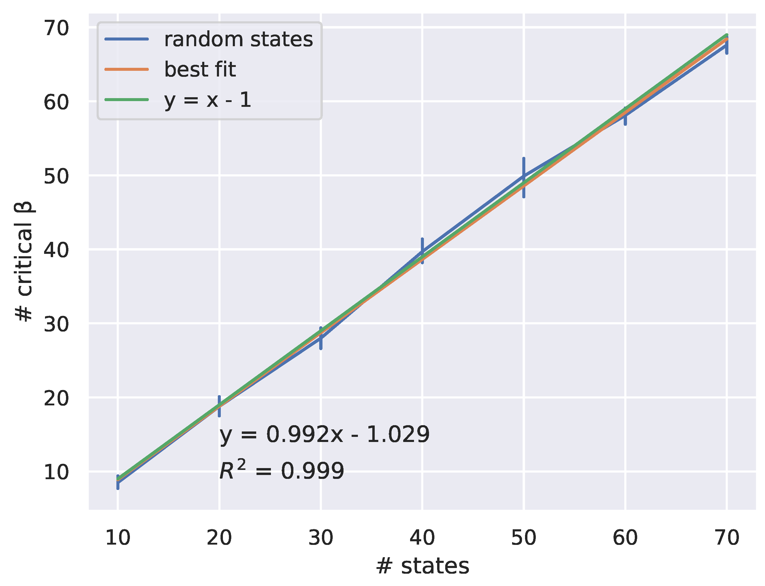
Figure 5.
Taking two random RD distributions D1 and D2 gives two RD curves which look similar, but whose critical points differ (points indicated along the curves), estimated from divergence rate maxima.
Figure 5.
Taking two random RD distributions D1 and D2 gives two RD curves which look similar, but whose critical points differ (points indicated along the curves), estimated from divergence rate maxima.
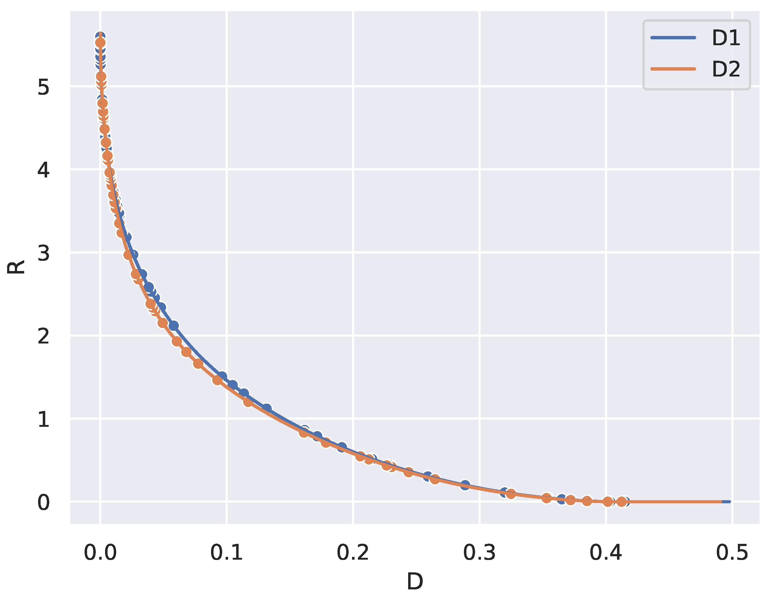
Figure 6.
RD curve and locations of critical codebooks for ON/OFF natural image patches (compare with [80]).
Figure 6.
RD curve and locations of critical codebooks for ON/OFF natural image patches (compare with [80]).
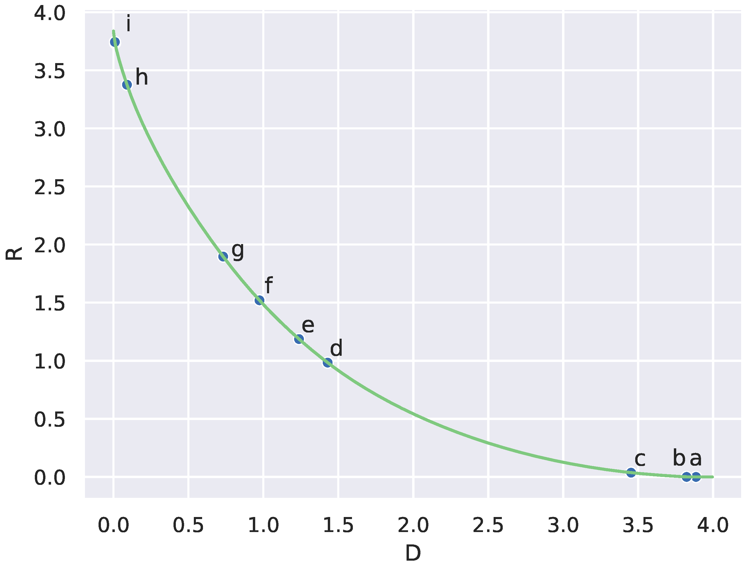
Figure 7.
Natural image patch codebooks at critical from Figure 6 estimated using divergence rate (compare with [80]). Each column represents the conditional distribution given an input state.
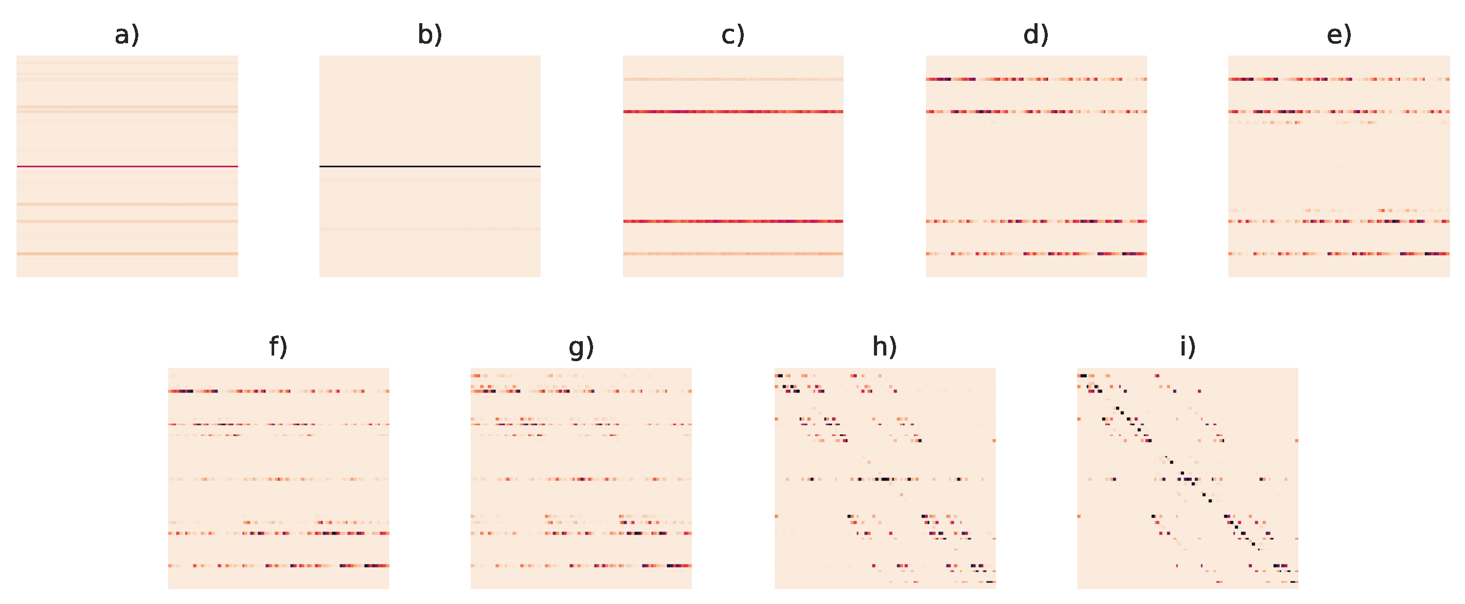
Figure 8.
Critical codebooks for clusters corresponding to critical points determined by peaks in divergence rate. Each column is the conditional distribution given an input state.
Figure 8.
Critical codebooks for clusters corresponding to critical points determined by peaks in divergence rate. Each column is the conditional distribution given an input state.

Figure 9.
Peaks in divergence rate suggest networks exhibit phase transitions along MEF learning.
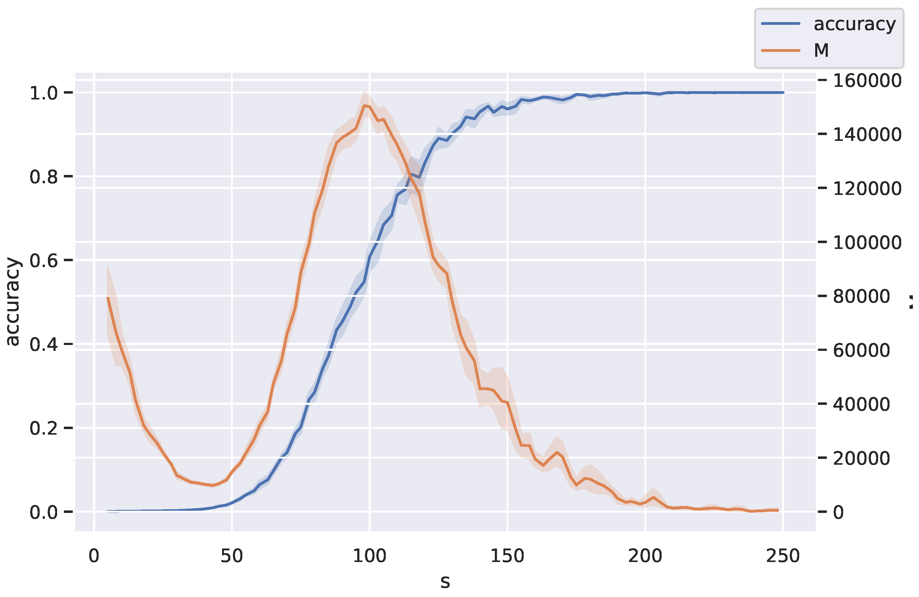
Figure 10.
a) Normalized plot of divergence rate for a horticultural journal corpus against time. b) Peaks along time in the corpus associated to the indicated words.
Figure 10.
a) Normalized plot of divergence rate for a horticultural journal corpus against time. b) Peaks along time in the corpus associated to the indicated words.
Disclaimer/Publisher’s Note: The statements, opinions and data contained in all publications are solely those of the individual author(s) and contributor(s) and not of MDPI and/or the editor(s). MDPI and/or the editor(s) disclaim responsibility for any injury to people or property resulting from any ideas, methods, instructions or products referred to in the content. |
© 2024 by the authors. Licensee MDPI, Basel, Switzerland. This article is an open access article distributed under the terms and conditions of the Creative Commons Attribution (CC BY) license (http://creativecommons.org/licenses/by/4.0/).
Copyright: This open access article is published under a Creative Commons CC BY 4.0 license, which permit the free download, distribution, and reuse, provided that the author and preprint are cited in any reuse.


