
Submitted:
11 May 2025
Posted:
13 May 2025
You are already at the latest version
Abstract
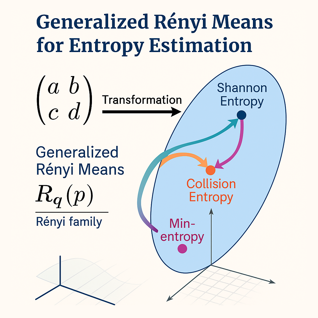
Rényi entropy is a generalization of Shannon entropy that enables the analysis of different aspects of the informative structure of probability distributions. This family of entropy measures is particularly valuable in scientific and technological contexts requiring the classification, comparison, or characterization of probability distributions, discrete stochastic processes, or discretized dynamical systems. Despite their theoretical appeal, Rényi entropies are challenging to estimate from empirical data—especially in settings involving limited samples, high dimensionality, or highly irregular behaviors. To address these difficulties, we propose a general-purpose estimation method applicable across the entire Rényi family. The method is based on affine transformations that enhance generality, robustness, and accuracy. In particular, the estimation of collision entropy achieves optimality in a single step. To help visualize and understand the effect of the transformation, we also introduce a geometric framework that represents probability distributions from the point of view of their entropic state. This provides intuitive insight into how our estimator works and why it is effective in practice.
Keywords:
estimation of Rényi entropies
1. Introduction
1.1. From Probability Theory to Information Theory
Probability theory plays a central role in modeling complex systems that operate under uncertainty. From Cardano’s early reflections on dice games of chance (De Ludo Aleae, ~1564) [1] and the correspondence between Fermat and Pascal on the problem posed by Pacioli (1654) [2], to Kolmogorov’s axiomatic formalization (1933) [3], the discipline of probability theory has gradually evolved from its heuristic origins into a mathematically rigorous and essential framework. Subsequently, information theory enabled a deeper exploration of the structure of probability distributions by using the concept of information entropy. Drawing inspiration from Boltzmann’s thermodynamic formulation, Shannon in 1948 [4] defined the entropy of a discrete probability distribution as
where denotes the probability of the event, and n is the number of possible outcomes. However, this fundamental quantity does not always distinguish between distributions with different internal structures. To address this limitation, Rényi in 1961 [5] introduced a parametric family of entropy measures, generalizing Shannon’s definition:
As , the Rényi entropy converges to the Shannon entropy, preserving theoretical consistency. Varying , the measure emphasizes different parts of the distribution, enabling finer structural analysis of probability distributions.
1.2. The Challenge of Accurate Entropy Estimation
Rényi’s axiomatic approach offered a flexible generalization with theoretical applications in communication theory [6,7], statistical mechanics [8,9], cryptography [10,11] and artificial intelligence [12,13]. However, estimating Rényi entropies from empirical data is difficult due to structural and statistical factors that compromise result reliability [14,15,16], including:
(a) Zero-frequency problem: rare events may be entirely absent from finite samples, leading to underestimated entropy—especially in heavy-tailed or sparse distributions;
(b) Paradox of data sparsity: as data become sparser in the sample space, the chance of observing all outcomes in correct relative proportions declines, paradoxically shrinking the empirical entropy even as statistical unreliability increases;
(c) Amplification of errors: Entropy’s nonlinear dependence on probabilities means that small empirical errors can be magnified, yielding high variance and instability;
(d) Curse of dimensionality: as the dimensionality increases, the event space grows exponentially, making data sparse and many outcomes rare or unobserved;
(e) Sensitivity to outliers and noise: anomalous events or random fluctuations can distort frequencies and cause erratic entropy values.
These challenges are particularly acute in small-sample regimes, high-dimensional settings, and data derived from high-entropy processes—all common in modern data analysis. As a result, even well-established estimation techniques often produce biased or unstable results.
1.3. Related Works and Previous Contributions
The estimation of members of the family of Rényi entropies—including Shannon entropy (), collision entropy (), and min-entropy ()—has been widely investigated and has garnered increasing attention due to its relevance in various applicative fields. Immediately after the invention of these indices, it was soon recognized that their naive plug-in estimators suffer from high bias and variance in small-sample or high-dimensional regimes. Later works proposed corrections and non-parametric models [17,18], though these remained limited in effectiveness. In response to these challenges, more efforts have progressively been directed toward developing increasingly sophisticated estimation methods: [10,15,16,19,20,21,22,23,24,25,26,27,28,29,30,31,32,33,34,35,36,37,38,39,40,41,42,43,44,45,46,47,48,49,50,51,52,53,54,55,56,57,58,59,60,61,62,63,64,65,66,67,68,69,70,71,72,73,74,75,76,77,78,79,80,81,82,83,84,85,86,87,88,89]. Despite these improvements, an universally recognized method capable of expressing optimal performance in any situation has not yet been achieved. Thus, in the continued absence of a definitive and unique procedure, the pursuit of a robust general-purpose estimator remains an open and central challenge in the study of Rényi entropies. It is also worth noting that, due to these difficulties, many researchers have proposed alternative indices, equipped with their customized estimators, such as Onicescu’s informational energy [90], approximate entropy [91], sample entropy [92], multiscale entropy [93], permutation entropy [94] and bubble entropy [95]. Beyond these isolated alternatives, one of the few comprehensive frameworks comparable in scope to the Rényi entropy family is the parametric family of Tsallis entropies [96], whose applicability is hindered by the lack of key properties such as additivity, scale invariance, and ease of normalization.
1.4. Motivation and Contribution of This Paper
This work is motivated by the persistent lack of a unified and widely accepted method for estimating Rényi entropies—a gap that has remained open for more than sixty years since their theoretical inception. We propose a novel method for the accurate estimation of Rényi entropies that requires minimal parameter tuning and can be used under diverse data conditions. The method effectively addresses the challenges mentioned in the previous paragraph. Empirical evidence confirms its performance in low-sample, high-dimensional, and high-entropy settings. At the core of the procedure lies an affine transformation1 applied to the empirical frequency distribution, introducing a structured geometric regularization whose overall effect is a global linear stretching. This transformation regularizes the geometry of the input space prior to the entropy computation, leading to an improved approximation of the true Rényi entropy via the Rényi mean2. This approach stems from the idea that the empirical entropies reside in a context that is different from the context of theoretical entropies and a transformation is necessary for the “translation” of these measures from one context to the other. The proposed transformation reorients and rescales the data in a principled manner, considerably reducing the estimation error for any entropy index and directly reaching the optimality for the case of (collision entropy).
2. Overview on Materials and Methods of Information Theory
2.1. Transforming a Discrete-State Stochastic Process into a Probability Distribution
Consider a discrete-state stochastic process () whose sequence of infinite samples presents values belonging to an alphabet containing q ordered symbols. Let be a d-dimensional discrete sample space resulting from the Cartesian product d times of .
and let be the cardinality of . Each elementary event , with , is uniquely identified by a vector with d coordinates (), with . According to the procedure indicated by Shannon in [4] at pages 5 and 6, the infinite sequence of samples constituting the can be transformed into occurrences of the elementary events of by progressively considering all the d-grams taken from the samples as if they were the vector coordinates of the events and counting the number of times each vector appears in the sequence. Then, according to the frequentist definition of probability, the final resulting probability distribution is expressible in set theory notation as
In the following, in the absence of ambiguity, —that is, a obtained by elaborating the data of a — will be indicated with the bold symbol and the probability of the event with .
2.2. Integer-Order Rényi -Entropies as Synthetic Indices for the Characterization of s
The family of integer-order Rényi -entropies offers synthetic indices that characterize s in terms of their informative content [5]. They are defined as:
The corresponding specific entropies are then defined as
Specific entropies are preferred over plain ones because:
(a) They range in via min-max normalization, which provides a unique bounded scale that greatly facilitates the interpretation of entropy values at any scale;
(b) They minimize the dependence on the sample space size n;
(c) They resolve doubts about the choice of the logarithm base, highlighting scale invariance;
(d) Entropies in base b are then given by .
2.3. Rényi Entropy Rates
Unlike Rényi entropies, whose utility is mainly related to the classification of s, Rényi entropy rates are important theoretical quantities useful for the characterization of s [61,72]; they are defined as
Moreover, it is known that, for strongly stationary , any Rényi entropy rate converges to the same limit of a sequence of Cesaro means of conditional entropies:
and, as conditional Rényi entropies preserve the chain rule [97,98,99], they can also be calculated as
Specific Rényi entropy rates are defined by the following min-max normalization:
with .
2.4. Relationship Between Specific Rényi Entropy Rate and Specific Rényi Entropy
2.5. Rényi Generalized Dimensions
Rényi entropies and their associated rates provide a unified framework for analyzing probability distributions and classifying stochastic processes. A closely related concept in multifractal analysis is the Rényi generalized dimension [100], defined as
where denotes a partition of the state space into d-dimensional cells of linear size , and is the probability that a trajectory of the dynamical system () crosses the i-th cell:
with denoting the number of visits in the i-th d-cell by the trajectory.
2.6. Rényi Generalized Dimension Rates
In analogy with entropy rates, we define the Rényi generalized dimension rate as
where is the Rényi entropy of order associated with the distribution induced by the partition.
Letting , the number of partition elements scales as . Since the specific Rényi entropy is defined as , the dimension rate becomes
Here, d is fixed, while q increases. To improve convergence and enable stable numerical estimation, we employ a differential formulation based on logarithmic increments:
2.7. Rényi Mutual Information
Another key quantity derived from -Rényi entropies is the -Rényi mutual information [48], defined for three random variables X, Y, and , with respective events , , and , and corresponding probability distributions , , and :
The corresponding expression in terms of specific entropy is:
2.8. Measures of Entropic Distance Between Distributions
Dissimilarity between two distributions A and B is often measured using Rényi divergences [101], of which the Kullback–Leibler divergence [102] (also known as relative entropy) is a special case. Since these divergences are not directly derived from Rényi entropies, we instead propose to measure their geometric distance in entropy space using the following formula:
where represents the number of entropy indices used to determine the state. This method provides a symmetric and broader generalization with respect to Rényi divergences, also allowing the comparison of distributions with different event-space cardinalities.
2.9. Two Fundamental Families of Structured Probability Distributions
To support controlled and interpretable experimentation, we define two fundamental families of structured probability distributions that form the basis of our experimental analysis. Designed to span the entire range of distributions over a finite alphabet, these families exhibit distinct structural properties that represent entropy extremes within the distribution space (see Figure 1 and Figure 2). They are:
- 1.
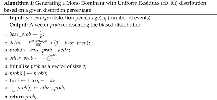
- Mono Dominant with Uniform Residues (MD_UR): This family generates distributions in which, starting from the uniform case, a single symbol progressively absorbs more probability mass by subtracting it uniformly from the other symbols. The family can be defined as:where the parameter controls the strength of the dominant symbol.
- 2.
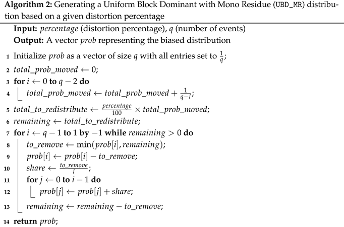
- Uniform Block Dominant with Mono Residue (UBD_MR): This family defines structured, biased distributions starting from a uniform base. Probability mass is progressively removed from the last non-zero event and equally redistributed among all preceding ones. The resulting distribution exhibits a dominant block of equal, high-probability values at the front, followed by a single lower residual value, with all subsequent entries set to zero. This construction induces a non-trivial truncation of the support and does not admit a simple closed-form expression.
For both families, explicit generation algorithms are provided to support reproducibility and controlled experimentation. These distributions define the entropic bounds that encompass all admissible shapes, from highly concentrated to nearly uniform. They are well suited to reveal how entropy estimators behave under structural constraints and will be used to benchmark performance, assess sensitivity, and identify systematic biases.
 |
 |
2.10. Ambiguity Reduction in Entropy-Based Measures
While a single entropy index provides valuable information, it may be insufficient to distinguish between probability distributions that share the same entropy value but differ in structural characteristics. This limitation can be addressed by combining multiple independent and complementary entropy indices—such as different Rényi entropies (e.g., Shannon entropy and collision entropy)—which enhance the ability to differentiate among distributions. For instance, for two distributions with identical Shannon entropy, the further observation of their collision entropy reveals structural differences that would otherwise remain hidden (see Figure 3).
2.11. Interpreting Rényi Entropies as the Negative Logarithm of Generalized Means
The generalized α-Hölder mean[103] of a discrete probability distribution over n elementary events is defined as:
This mean interpolates between classical means as varies: in fact is the harmonic mean, is the geometric mean, is the arithmetic mean, is the root mean square, is the mean considering the maximum value. Building on this idea, we define the generalized α-Rényi mean of a discrete probability distribution as:
Accordingly, the Rényi entropy of order can be expressed as:
Each order corresponds to a distinct generalized averaging scheme, providing insight into the distribution’s internal structure from complementary informational perspectives. This framework also recovers several well-known entropy measures as special cases:
Shannon entropy () from the Shannon mean:
3. Practical Implementation of Methods of Information Theory
This section addresses the transition from idealized models—based on exact knowledge of discrete probability distributions—to practical scenarios involving finite samples, where the true underlying distributions are unknown. By reformulating the theoretical framework in terms of observed relative frequencies, it enables inference and estimation of properties of the underlying generative process. This procedure is composed of three steps: (a) Determining relative frequencies from samples;
(b) Calculating apparent Rényi means/entropies of the relative frequencies;
(c) Inferring the actual Rényi means/entropies of the underlying probability distribution.
3.1. Converting a Realization into a Relative Frequency Distribution
In practical applications, the theoretical procedure described in § Section 2.1 can be adapted as follows: consider the L samples of a realization r, extracted from a represented using q ordered symbols. Each d-gram, consisting of d consecutive samples from r, is treated as the occurrence of an elementary event in the d-dimensional sample space , where each d-gram defines a unique vector in this space. For example, the first two d-grams taken from , and identify the first occurrences of two elementary events. The count of the occurrences of events is performed for all the d-grams progressively identified in the sequence of the samples of r. The absolute frequency of each elementary event is normalized by the total number of occurrences, (), yielding the corresponding relative frequency . The final resulting is expressible in set theory notation as
where represents the total number of observed d-grams. For brevity, when there is no risk of ambiguity, an RFD derived from a realization within a given sample space will be denoted simply as , and represents the relative frequency attributed to the event.
3.2. Rényi Mean and Specific Rényi Entropy of a Relative Frequency Distribution
For a relative frequency distribution, the empirical Rényi mean is defined as:
Consequently, the empirical specific Rényi entropy results
3.3. Apparent vs. Actual Specific Entropies in Controlled Probabilistic Processes
Figure 4 and Figure 5 show the result of the comparison of theoretical and empirical specific entropies for the two previously introduced limit families of discrete probability distributions, MD_UR and UBD_MR. Three theoretical indices, , , and , are placed in relationship each with its empirical counterpart, respectively , , and , calculated from relative frequencies. Each family includes 100 synthetic processes, generated by progressively deforming a fair die distribution () into a degenerate one (), with a distortion percentage increasing from to along its entropic path. For each theoretical distribution, realizations (each samples long) are produced, and event samples are drawn in a dimensional space (), resulting in a sparse data regime (data density ). As distortion grows, both true and empirical entropies decrease, but empirical estimates systematically underestimate true values, especially near uniformity. Saturation sets in beyond the threshold , highlighted in the figures by a vertical dashed line, where the empirical entropy is restricted by the limited number of observed data. Despite construction differences, both families exhibit similar transitions from uniformity to concentration, highlighting common limitations of entropy estimation under finite sampling. Thus, these models provide a controlled framework for studying the interaction between distribution structure, sparsity, and estimation reliability, providing insights for high-dimensional inference.
3.4. Determination of the Relationship Between Actual and Apparent Rényi Mean
To enable a meaningful comparison between actual Rényi mean (based on the true distribution ) and apparent Rényi mean (computed from empirical frequencies ), it is convenient to apply a min-max normalization to both quantities using their respective minimal and maximal attainable values. These transformations give two comparable quantities, both ranging in interval:
The second normalization assumes that when the true entropy is maximal—that is, when —the apparent Rényi mean reaches its minimum value of exactly . However, empirical evidence—as shown in Figure 4, Figure 5—suggests otherwise: the minimum value of the apparent Rényi mean under maximum entropy conditions can deviate from and this deviation is maximal for .
To account for this discrepancy, we introduce the term , which represents the empirical lower bound of the -Rényi mean. It is computed as the average value of the Rényi mean over multiple realizations drawn from a perfectly uniform process, governed by a perfectly uniform distribution (U)—i.e., one with maximal specific entropy—under the same sampling conditions .
This empirically refined mean minimum, specific to each triplet , is defined as:
- is the scaling factor;
- is the translation offset;
3.5. Toward Accurate Estimation of Rényi Entropies via Affine Transformations
The affine structure of (32) suggests a possible interpretation of the estimator: it maps the apparent internal state of the distribution (observed empirically from relative frequencies) into its actual internal state (in the theoretical context of probabiity distributions). The Rényi entropy itself () can thus be interpreted as an observable readout of this internal state. Based on equation (31), the estimated specific Rényi entropy is:
This expression holds for all , including limiting cases such as Shannon entropy () and min-entropy (). This approach yields a non-iterative, scalable, and theoretically grounded estimator. Its derivation is based on:
- Min-max normalization of actual and empirical Rényi means, to ensure comparability;
- A linear transformation between the two domains;
- The logarithmic relationship between Rényi entropy and Rényi mean.
By integrating these elements, the estimator provides a principled way to recover the entropy of the underlying process from observed frequencies, based on the following properties:
- 1.
- Change of paradigm: data do not need correction, but they have to be rescaled from an empirical to a theoretical context.
- 2.
- Consistency: as , we have and , ensuring that converges to the true entropy .
- 3.
- Bias and variance control: the estimator compensates for the known bias in empirical frequencies by incorporating a prior empirical mean , resulting in a lower mean squared error compared to classical estimators.
- 4.
- Computational efficiency: the formula requires only a few arithmetic operations and, optionally, a numerically precomputed lookup table for , making it suitable for large-scale inference.
The left column of Figure 6 consolidates the results previously shown in the left panels of Figure 4 and Figure 5, reorganizing the same data into separate plots by entropy type: specific Shannon entropy at the top, specific collision entropy in the middle, and specific min-entropy at the bottom. For each entropy type, the results obtained from the MD_UR and UBD_MR distribution families define a region that encloses all points achievable by applying the same procedures to any probability distribution under identical sampling conditions () and sample space structure (). The right column of Figure 6 illustrates the effect of applying formula (33) to the data, which induces a geometric transformation that diagonally stretches the region representing the relationship between the entropy of theoretical and empirical distributions. In the specific case of collision entropy, this transformation causes the curves associated with all distribution families—from MD_UR to UBD_MR—to nearly coincide with the diagonal line (see central panel in Figure 6). As a result, this transformation alone completes the estimation procedure for specific collision entropy. In contrast, the estimation of other Rényi entropies, such as Shannon and min-entropy, requires an additional adjustment step to reach comparable accuracy.
As a result, the specific collision entropy emerges as the most coherent index. Moreover, its optimal estimation can be performed with a single transformation. For this reason, it will serve as the horizontal reference axis in subsequent diagrams, facilitating comparative assessments of the estimators of other entropies. Using this approach, the data from Figure 6 can be recomposed by plotting the specific collision entropy on the X-axis and mapping on the left Y-axis and on the right Y-axis of the diagram, respectively. The outcome of this new composition is shown in Figure 7.
3.6. A Second Transformation for More Accurate Estimation of Entropies: Orthogonal Stretch
While the diagonal stretch is sufficient for accurately estimating the specific collision entropy, it proves inadequate for other Rényi entropies. As illustrated in Figure 7, this affine transformation alone fails to fully map the region derived from empirical data onto the corresponding region defined by theoretical probability distributions. To overcome this limitation, a second transformation—orthogonal to the direction associated with the collision mean—is required to complete the geometric alignment. A detailed analysis of this additional step, which represents a further advancement toward accurate Rényi entropy estimation, lies beyond the scope of the present work, which primarily serves as an introduction to this novel approach.
3.7. A Practical Example of Applying the First Order Affine Transformation
In this example, we demonstrate how the entropic state of a can be recovered from a set of short realizations sampled from the process defined by the original . The recovery is carried out by applying the previously described first-order affine transformation to the generalized means of empirical data distributions. Its procedure consists of the following steps:
- 1.
- Choice of the stochastic process: In this case, without loss of generality, and following the foundational approach adopted by early pioneers of probability theory (e.g., Cardano, Galileo, Pascal, Fermat, Huygens, Bernoulli, de Moivre, Newton), we consider a memoryless stochastic process generated by repeated rolls of a six-sided die subject to a specific probability distribution. The key advantage of using memoryless processes is that their entropic state remains invariant under changes in the dimensionality of the sample space used for statistical analysis.
- 2.
- Choice of the theoretical : We select a distribution whose entropic characteristics lie far from the regions typically covered by empirical distributions derived from small samples, thereby making the recovery task more challenging, for instance:
- 3.
- Choice of the composition of the entropic space: We consider a three dimensional entropic space. The entropies are: specific Shannon entropy (), specific collision entropy (), and specific min-entropy (). A generic three-dimensional point is projected onto two two-dimensional points: , located above the diagonal in the collision entropy-Shannon entropy plane (blue zone), and , located beneath the diagonal in the collision entropy-min-entropy plane (red zone). The value of is shared between the two projections.
- 4.
- Visualization of theoretical, empirical, and stretched contexts: To clearly distinguish the regions concerning the states of theoretical probability distributions, of their derived empirical distributions, and of the states resulting after the application of the first-order affine transformation, the diagram includes the curves generated by the elaborations over MD_UR and UBD_MR families, along with the curves relative to the corresponding realizations and their stretched versions.
- 5.
- Determination of the entropic state points of the theoretical distribution T: These points describe the entropic state of the initial distribution and represent the target of the estimation process:
- 6.
- Generation of realizations: A set of realizations is generated from the process by applying a random number generator to the previously defined probability distribution T. A large number of realizations helps reduce the deviation of the final estimation from the target value. Each realization consists of a sequence of samples.
- 7.
- Choice of the the parameters of the sample space Ω: To significantly reduce the density of data, we select a sample space with the same alphabet of the process and dimension . The total number of elementary events is .
- 8.
- Embedding data into the sample space to derive relative frequencies: Consequently, the number of elementary events that occur in is . This leads to a very sparse data regime, with a density .
- 9.
- Calculation of their center of gravity S: For each realization, we compute the Rényi means and their logarithmic mapping in entropy plane; the results are then averaged:
- 10.
- Calculation of their center of gravity E: The affine transformation is applied to the Rényi means of the empirical data and the entropic state points of the translated Rényi means are derived; the results are then averaged:
- 11.
- Evaluation of the distance between E and T: The estimation method is satisfying when point E results coincident or very near to point T
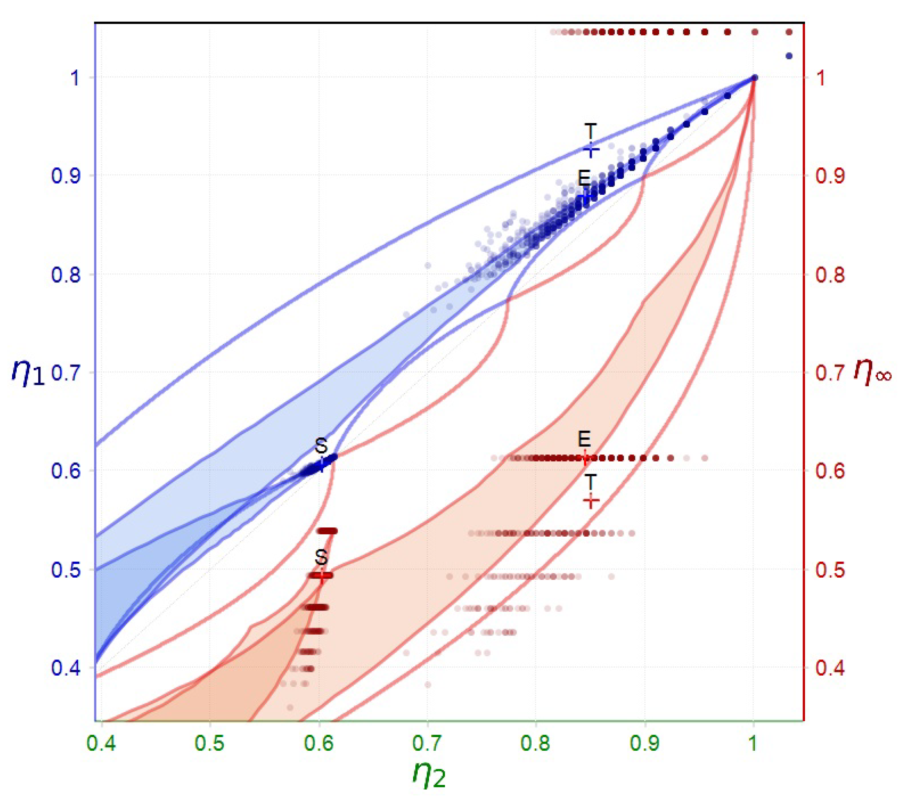
Figure 8 illustrates the effect of the previous steps.
4. Discussion
4.1. Considerations on the Example Presented in § 3.7
The example in § 3.7 illustrates a typical scenario where the entropic state of a theoretical distribution T significantly diverges from the empirical state S, derived from relative frequencies. Directly using values from S to estimate T would thus lead to substantial errors. Applying the affine transformation (31) to the Rényi generalized means computed from data yields entropy estimates defining a new state E, much closer to T. The collision entropy of E closely matches T, whereas the Shannon and min-entropy estimates show larger discrepancies, highlighting the need for further adjustments. Moreover, empirical points appearing clustered become more dispersed after transformation, indicating an increase in variance. Given that the value of in this example is computed from a great number fo realizations, applying it to a smaller set (e.g., realizations) might produce state points exceeding , particularly for min-entropy.
4.2. Considerations Concerning Algorithms for Generating MD_UR and UBD_MR Families of s
To explore entropy trends in controlled distributions, we developed two algorithms: one for Mono Dominant with Uniform Residues (MD_UR) and another for Uniform Block Dominant with Mono Residue (UBD_MR), both derived from a uniform baseline by applying increasing distortion percentages. Algorithm 1 (MD_UR) is straightforward, with linear complexity , involving a single pass over events. Algorithm 2 (UBD_MR), however, redistributes probability from the tail to the head using nested loops and conditional logic, resulting in quadratic complexity . Thus, steering distributions toward Algorithm 1’s path is computationally simpler than compressing them via Algorithm 2, reflecting intrinsic asymmetries in entropy landscapes that could impact the modeling of natural probabilistic processes.
4.3. Data Contextualization vs. Data Correction in Entropy Estimation Methods
Another insight is a relativistic reinterpretation of relative frequencies in entropy estimation. Instead of viewing these frequencies as biased or erroneous, we suggest considering them as geometrically constrained observations. Limited dataset size naturally compresses empirical frequencies within the entropy state space. The affine transformation of Rényi generalized means thus acts not as traditional correction but as geometric re-contextualization, stretching empirical observations to align them with the theoretical entropy structure. This interpretation parallels general relativity’s insight that mass shapes spacetime: data mass similarly shapes observable entropy space. Small datasets produce compressed entropy states, which expand toward theoretical configurations as data mass increases. Figure 7 clearly visualizes this phenomenon, showing initial empirical compression and subsequent geometric expansion via affine transformation and logarithmic mapping.
5. Conclusion
In a broad sense, this work aims to contribute to answer to Hilbert’s Sixth Problem by addressing the longstanding challenge of rigorously bridging axiomatic foundations and empirical methodologies. It proposes a novel entropy estimator, grounded in a structured affine transformation of empirical frequency distributions, effectively translating formal definitions of Rényi entropy into practical, statistically robust and computationally efficient estimation methods. The paper introduces three core innovations: (1) the use of specific entropies , enabling clear geometric interpretations; (2) the definition of two structured probability distribution families—Mono Dominant with Uniform Residues (MD_UR) and Uniform Block Dominant with Mono Residue (UBD_MR); and (3) a general estimation framework applicable across varying datasets, data types, and dimensions, capable of accurately estimating Shannon, collision, and min-entropy. Among these, collision entropy stands out because of its simplicity of estimation via affine stretching. However, relying solely on collision entropy can obscure critical nuances. Thus, the proposed approach naturally encourages the complementary use of multiple entropy indices (collision, Shannon, and min-entropy), enriching the characterization of uncertainty. Furthermore, this framework offers rigorous epistemological insights by precisely quantifying how empirical data contribute to our understanding of underlying realities.
6. Future Work
The findings of this study suggest several future research directions:
- Improved transformation models: Develop secondary orthogonal transformations to refine entropy estimation, especially min-entropy, through adaptive corrections.
- Analytical characterization and simplification: Investigating analytical approximations or tight bounds for empirical Rényi means , reducing computational complexity.
- Variance control and confidence estimation: Enhancing robustness by exploring variance control methods, including smoothing kernels, shrinkage techniques, or deriving confidence intervals analytically.
- Extension to real-world data: Validation of the estimator on real datasets, particularly in cybersecurity, neuroscience, and computational biology, to test practical effectiveness.
- Generalization to other information functionals: Extending the affine estimation framework to broader information-theoretic measures, expanding its theoretical and practical scope.
- Integration into statistical and machine learning workflows: Exploring applications of entropy estimation within machine learning as feature transformations, loss functions, or regularizers to innovate data-driven modeling.
Funding
This research received no external funding. Commercial licensing of the entropy estimation algorithms described in this work can be arranged by contacting the author.
Conflicts of Interest
The author declares no conflicts of interest.
Abbreviations
The following abbreviations are used in this manuscript:
| Set of q ordered symbols (alphabet) | |
| Stationary, infinite length, discrete-state stochastic process whose samples | |
| belong to | |
| r | Physical realization (data sequence of finite length) taken from a |
| L | Number of samples constituting r |
| Set of physical realizations | |
| Arithmetic mean of calculated over | |
| Sample space resulting from the Cartesian product d times of | |
| d | Dimension of |
| Cardinality of | |
| Number of occurrences of elementary events of observed during the | |
| evolution of r | |
| Data density in the sample space | |
| Discrete probability distribution | |
| MD_UR | Mono Dominant (with Uniform Residues) family of s |
| UBD_MR | Uniform block dominant (with Mono Residue) family of s |
| Relative frequency distribution | |
| obtained from a whose infinite d-grams are considered coordinates | |
| of occurred elementary events of | |
| obtained from a realization r whose finite d-grams are considered | |
| coordinates of occurred elementary events of | |
| Order of a Rényi mean or of a Rényi entropy | |
| -Rényi mean of a | |
| -Rényi mean of a | |
| Estimated -Rényi mean of a | |
| -Rényi entropy of a | |
| -Rényi entropy of a | |
| Specific -Rényi entropy of a | |
| Specific -Rényi entropy of an | |
| Estimated specific Rényi -entropy of a | |
| Specific Rényi -entropy rate of a | |
| Specific Rényi -entropy rate of r | |
| Estimated specific Rényi -entropy rate of a | |
| Dynamical system | |
| Partition of the state space into d-dimensional cells of linear size | |
| Probability that a trajectory of the crosses the i-th cell | |
| Rényi generalized dimension of order | |
| Rényi Generalized Dimension Rate of order of the | |
| -Rényi mutual information | |
| Specific -Rényi mutual information |
| 1 |
An affine transformation is a mapping of the form , where A is a linear operator (e.g., a matrix) and B is a fixed vector. It preserves points, straight lines, and planes, and includes operations such as scaling, rotation, translation, and shear. |
| 2 | The Rényi mean of order of a probability distribution is a generalized averaging operator defined as . It forms the basis of Rényi entropy, which is defined as . |
References
- Cardano, G. Liber de Ludo Aleae (The Book on the Game of DiceGames of Chance); 1564. Published posthumously in 1663.
- Pascal, B.; de Fermat, P. Correspondence on the Problem of Points; Original correspondence, Toulouse and Paris, 1654. Reprinted and translated in various historical anthologies on the foundations of probability theory.
- Kolmogorov, A. Foundations of the theory of probability, 1950 ed.; Chelsea Publishing Co.: New York, 1933. [Google Scholar]
- Shannon, C. A mathematical theory of communication. The Bell System Technical Journal 1948, 27, 379–423. [Google Scholar] [CrossRef]
- Rényi, A. On measures of entropy and information. In Proceedings of the Proceedings of the Fourth Berkeley Symposium on Mathematical Statistics and Probability, Volume 1: Contributions to the Theory of Statistics, Berkeley, CA, USA, 1961; pp.547–561.
- Arikan, E. An inequality on guessing and its application to sequential decoding. In Proceedings of the Proceedings of 1995 IEEE International Symposium on Information Theory, 1995, pp. 322–. [CrossRef]
- Csiszár, I. Generalized cutoff rates and Rényi’s information measures. IEEE Transactions on information theory 1995, 41, 26–34. [Google Scholar] [CrossRef]
- Beck, C. Generalised information and entropy measures in physics. Contemporary Physics 2009, 50, 495–510. [Google Scholar] [CrossRef]
- Fuentes, J.; Gonçalves, J. Rényi Entropy in Statistical Mechanics. Entropy 2022, 24. [Google Scholar] [CrossRef]
- Cachin, C. Smooth entropy and Rényi entropy. In Proceedings of the International Conference on the Theory and Applications of Cryptographic Techniques. Springer; 1997; pp. 193–208. [Google Scholar]
- Boztas, S. On Rényi entropies and their applications to guessing attacks in cryptography. IEICE Transactions on Fundamentals of Electronics, Communications and Computer Sciences 2014, 97, 2542–2548. [Google Scholar] [CrossRef]
- Badhe, S.S.; Shirbahadurkar, S.D.; Gulhane, S.R. Renyi entropy and deep learning-based approach for accent classification. Multimedia Tools and Applications 2022, pp. 1–33.
- Sepúlveda-Fontaine, S.A.; Amigó, J.M. Applications of Entropy in Data Analysis and Machine Learning: A Review. Entropy 2024, 26. [Google Scholar] [CrossRef] [PubMed]
- Pál, D.; Póczos, B.; Szepesvári, C. Estimation of Rényi entropy and mutual information based on generalized nearest-neighbor graphs. Advances in neural information processing systems 2010, 23. [Google Scholar]
- Acharya, J.; Orlitsky, A.; Suresh, A.; Tyagi, H. The Complexity of Estimating Rényi Entropy. In Proceedings of the The twenty-sixth annual ACM-SIAM Symposium on Discrete Algorithms, SODA 2015, San Diego, CA, USA, January 4-6 2015. SIAM, SIAM, 2015; pp. 1855–1869. [CrossRef]
- Skorski, M. Practical Estimation of Renyi Entropy, 2020, [arXiv:cs.DS/2002.09264]. arXiv:cs.DS/2002.09264].
- Miller, G.A. Note on the bias of information estimates. Information Theory in Psychology, 1955; II-B, 95–100. [Google Scholar]
- Vasicek, O.A. A Test for Normality Based on Sample Entropy. Journal of the Royal Statistical Society: Series B (Methodological) 1976, 38, 54–59. [Google Scholar] [CrossRef]
- Basharin, G.P. On a statistical estimate for the entropy of a sequence of independent random variables. Theory Probab. Appl. 1959, 4, 333–336. [Google Scholar] [CrossRef]
- Good, I. Maximum entropy for hypothesis formulation, especially for multidimensional contingency tables. Ann. Math. Statist. 1963, 34, 911–934. [Google Scholar] [CrossRef]
- Harris, B. The statistical estimation of entropy in the non-parametric case. Mathematics Research Center – Technical Summary Report 1975.
- Grassberger, P.; Procaccia, I. Estimation of the Kolmogorov entropy from a chaotic signal. Phys. Rev. A 1983, 28, 2591–2593. [Google Scholar] [CrossRef]
- Akaike, H. Prediction and entropy. In Selected Papers of Hirotugu Akaike; Springer, 1985; pp. 387–410.
- Kozachenko, L.F.; Leonenko, N.N. Sample Estimate of the Entropy of a Random Vector. Problemy Peredachi Informatsii 1987, 23:2, 95––101.
- Grassberger, P. Finite sample corrections to entropy and dimension estimates. Physics Letters A 1988, 128, 369–373. [Google Scholar] [CrossRef]
- Joe, H. Estimation of Entropy and Other Functionals of a Multivariate Density. Annals of the Institute of Statistical Mathematics 1989, 41, 683–697. [Google Scholar] [CrossRef]
- Hall, P.; Morton, S. On the estimation of entropy. Annals of the Institute of Statistical Mathematics 1993, 45, 69–88. [Google Scholar] [CrossRef]
- Wolpert, D.; Wolf, D. Estimating functions of probability distributions from a finite set of samples. Phys. Rev. E 1995, 52, 6841–6854. [Google Scholar] [CrossRef] [PubMed]
- Pöschel, T.; Ebeling, W.; Rosé, H. Guessing probability distributions from small samples. Journal of Statistical Physics 1995, 80, 1443–1452. [Google Scholar] [CrossRef]
- Schürmann, T.; Grassberger, P. Entropy estimation of symbol sequences. Chaos: An Interdisciplinary Journal of Nonlinear Science 1996, 6, 414–427. [Google Scholar] [CrossRef]
- Paluš, M. Coarse-grained entropy rates for characterization of complex time series. Physica D: Nonlinear Phenomena 1996, 93, 64–77. [Google Scholar] [CrossRef]
- Panzeri, S.; Treves, A. Analytical estimates of limited sampling biases in different information measures. Network: Computation in Neural Systems 1996, 7, 87–107. [Google Scholar] [CrossRef]
- Beirlant, J.; Dudewicz, E.; Györfi, L.; Denes, I. Nonparametric entropy estimation. An overview. 1997, Vol. 6, pp. 17–39.
- Schmitt, A.; Herzel, H. Estimating the Entropy of DNA Sequences. Journal of theoretical biology 1997, 188, 369–77. [Google Scholar] [CrossRef]
- Strong, S.P.; Koberle, R.; de Ruyter van Steveninck, R.R.; Bialek, W. Entropy and Information in Neural Spike Trains. Phys. Rev. Lett. 1998, 80, 197–200. [Google Scholar] [CrossRef]
- Porta, A.; Baselli, G.; Liberati, D.; Montano, N.; Cogliati, C.; Gnecchi-Ruscone, T.; Malliani, A.; Cerutti, S. Measuring regularity by means of a corrected conditional entropy in sympathetic outflow. Biological cybernetics 1998, 78, 71–8. [Google Scholar] [CrossRef] [PubMed]
- Holste, D.; Große, I.; Herzel, H. Bayes’ estimators of generalized entropies. Journal of Physics A: Mathematical and General 1998, 31, 2551–2566. [Google Scholar] [CrossRef]
- Chen, S.; Goodman, J. An empirical study of smoothing techniques for language modeling. Computer Speech & Language 1999, 13, 359–394. [Google Scholar]
- de Wit, T.D. When do finite sample effects significantly affect entropy estimates? The European Physical Journal B - Condensed Matter and Complex Systems 1999, 11, 513–516. [Google Scholar] [CrossRef]
- Rached, Z.; Alajaji, F.; Campbell, L.L. Rényi’s entropy rate for discrete Markov sources. In Proceedings of the Proceedings of the CISS, 1999, Vol. 99, pp. 17–19.
- Antos, A.; Kontoyiannis, I. Convergence properties of functional estimates for discrete distributions. Random Structures & Algorithms 2001, 19, 163–193. [Google Scholar] [CrossRef]
- Nemenman, I.; Shafee, F.; Bialek, W. Entropy and inference, revisited. In T. G. Dietterich, S. Becker, and Z. Ghahramani, editors, Advances in Neural Information Processing Systems 2002, 14, 471–478. [Google Scholar]
- Chao, A.; Shen, T.J. Non parametric estimation of Shannon’s index of diversity when there are unseen species. Environ. Ecol. Stat. 2003, 10, 429–443. [Google Scholar] [CrossRef]
- Grassberger, P. Entropy estimates from insufficient samples. arXiv2003, physics/0307138v2 2003.
- Paninski, L. Estimation of entropy and mutual information. Neural Computation 2003, 15, 1191–1253. [Google Scholar] [CrossRef]
- Wyner, A. ; D., F. On the lower limits of entropy estimation. IEEE Transactions on Information Theory - TIT.
- Amigó, J.M.; Szczepański, J.; Wajnryb, E.; Sanchez-Vives, M.V. Estimating the Entropy Rate of Spike Trains via Lempel-Ziv Complexity. Neural Computation 2004, 16, 717–736. [Google Scholar] [CrossRef]
- Kraskov, A.; Stögbauer, H.; Grassberger, P. Estimating mutual information. Phys. Rev. E 2004, 69, 066138. [Google Scholar] [CrossRef] [PubMed]
- Paninski, L. Estimating entropy on m bins given fewer than m samples. IEEE Transactions on Information Theory 2004, 50, 2200–2203. [Google Scholar] [CrossRef]
- Pöschel, T.; Ebeling, W.; Frömmel, C.; Ramirez, R. Correction algorithm for finite sample statistics. The European physical journal. E, Soft matter 2004, 12, 531–41. [Google Scholar] [CrossRef] [PubMed]
- Schürmann, T. Bias analysis in entropy estimation. Journal of Physics A: Mathematical and General 2004, 37, L295. [Google Scholar] [CrossRef]
- Ciuperca, G.; Girardin, V. On the estimation of the entropy rate of finite Markov chains. In Proceedings of the Proceedings of the international symposium on applied stochastic models and data analysis, 2005, pp.1109–1117.
- Szczepański, J.; Wajnryb, E.; Amigó, J.M. Variance Estimators for the Lempel-Ziv Entropy Rate Estimator. Chaos: An Interdisciplinary Journal of Nonlinear Science 2006, 16, 043102. [Google Scholar] [CrossRef]
- Hlaváčková-Schindler, K.; Paluš, M.; Vejmelka, M.; Bhattacharya, J. Causality detection based on information-theoretic approaches in time series analysis. Physics Reports 2007, 441, 1–46. [Google Scholar] [CrossRef]
- Kybic, J. High-Dimensional Entropy Estimation for Finite Accuracy Data: R-NN Entropy Estimator. In Proceedings of the Information Processing in Medical Imaging; Karssemeijer, N.; Lelieveldt, B., Eds., Berlin, Heidelberg; 2007; pp. 569–580. [Google Scholar]
- Vu, V.; Yu, B.; Kass, R. Coverage-adjusted entropy estimation. Statistics in Medicine 2007, 26, 4039–4060. [Google Scholar] [CrossRef]
- Bonachela, J.; Hinrichsen, H.; Muñoz, M. Entropy estimates of small data sets. Journal of Physics A: Mathematical and Theoretical 2008, 41, 9. [Google Scholar] [CrossRef]
- Grassberger, P. Entropy Estimates from Insufficient Samplings, 2008, [arXiv:physics.data-an/physics/0307138].
- Hausser, J.; Strimmer, K. Entropy inference and the James-Stein estimator, with application to nonlinear gene association networks. J. Mach. Learn. Res. 2009, 10, 1469–1484. [Google Scholar]
- Lesne, A.; Blanc, J.; Pezard, L. Entropy estimation of very short symbolic sequences. Physical Review E 2009, 79, 046208. [Google Scholar] [CrossRef]
- Golshani, L.; Pasha, E.; Yari, G. Some properties of Rényi entropy and Rényi entropy rate. Information Sciences 2009, 179, 2426–2433. [Google Scholar] [CrossRef]
- Xu, D.; Erdogmuns, D. , Divergence and Their Nonparametric Estimators. In Information Theoretic Learning: Renyi’s Entropy and Kernel Perspectives; Springer New York: New York, NY, 2010; pp. 47–102. [Google Scholar] [CrossRef]
- Källberg, D.; Leonenko, N.; Seleznjev, O. Statistical Inference for Rényi Entropy Functionals. arXiv preprint arXiv:1103.4977 2011.
- Nemenman, I. Coincidences and Estimation of Entropies of Random Variables with Large Cardinalities. Entropy 2011, 13, 2013–2023. [Google Scholar] [CrossRef]
- Vinck, M.; Battaglia, F.; Balakirsky, V.; Vinck, A.; Pennartz, C. Estimation of the entropy based on its polynomial representation. Phys. Rev. E 2012, 85, 051139. [Google Scholar] [CrossRef] [PubMed]
- Boucheron, S.; Lugosi, G.; Massart, P. Concentration Inequalities: A Nonasymptotic Theory of Independence; Vol. 14, Oxford Series in Probability and Statistics, Oxford University Press: Oxford, UK, 2013. Focuses on concentration inequalities with applications in probability, statistics, and learning theory.
- Zhang, Z.; Grabchak, M. Bias Adjustment for a Nonparametric Entropy Estimator. Entropy 2013, 15, 1999–2011. [Google Scholar] [CrossRef]
- Valiant, G.; Valiant, P. Estimating the Unseen: Improved Estimators for Entropy and Other Properties. J. ACM 2017, 64. [Google Scholar] [CrossRef]
- Li, L.; Titov, I.; Sporleder, C. Improved estimation of entropy for evaluation of word sense induction. Computational Linguistics 2014, 40, 671–685. [Google Scholar] [CrossRef]
- Archer, E.; Park, I.; Pillow, J. Bayesian entropy estimation for countable discrete distributions. The Journal of Machine Learning Research 2014, 15, 2833–2868. [Google Scholar]
- Schürmann, T. A Note on Entropy Estimation. Neural Comput. 2015, 27, 2097–2106. [Google Scholar] [CrossRef]
- Kamath, S.; Verdú, S. Estimation of entropy rate and Rényi entropy rate for Markov chains. In Proceedings of the 2016 IEEE International Symposium on Information Theory (ISIT); 2016; pp. 685–689. [Google Scholar] [CrossRef]
- Skorski, M. Improved estimation of collision entropy in high and low-entropy regimes and applications to anomaly detection. Cryptology ePrint Archive, Paper 2016/1035, 2016.
- Acharya, J.; Orlitsky, A.; Suresh, A.; Tyagi, H. Estimating Rényi entropy of discrete distributions. IEEE Transactions on Information Theory 2017, 63, 38–56. [Google Scholar] [CrossRef]
- de Oliveira, H.; Ospina, R. A Note on the Shannon Entropy of Short Sequences 2018. [CrossRef]
- Berrett, T.; Samworth, R.; Yuan, M. Efficient multivariate entropy estimation via k-nearest neighbour distances. The Annals of Statistics 2019, 47, 288–318. [Google Scholar] [CrossRef]
- Verdú, S. Empirical estimation of information measures: a literature guide. Entropy 2019, 21, 720. [Google Scholar] [CrossRef] [PubMed]
- Goldfeld, Z.; Greenewald, K.; Niles-Weed, J.; Polyanskiy, Y. Convergence of smoothed empirical measures with applications to entropy estimation. IEEE Transactions on Information Theory 2020, 66, 4368–4391. [Google Scholar] [CrossRef]
- Kim, Y.; Guyot, C.; Kim, Y. On the efficient estimation of Min-entropy. IEEE Transactions on Information Forensics and Security 2021, 16, 3013–3025. [Google Scholar] [CrossRef]
- Contreras Rodríguez, L.; Madarro-Capó, E.; Legón-Pérez, C.; Rojas, O.; Sosa-Gómez, G. Selecting an effective entropy estimator for short sequences of bits and bytes with maximum entropy. Entropy 2021, 23. [Google Scholar] [CrossRef]
- Ribeiro, M.; Henriques, T.; Castro, L.; Souto, A.; Antunes, L.; Costa-Santos, C.; Teixeira, A. The entropy universe. Entropy 2021, 23. [Google Scholar] [CrossRef] [PubMed]
- Subramanian, S.; Hsieh, M.H. Quantum algorithm for estimating alpha-Rényi entropies of quantum states. Physical Review A 2021, 104, 022428. [Google Scholar] [CrossRef]
- Grassberger, P. On Generalized Schürmann Entropy Estimators. Entropy 2022, 24. [Google Scholar] [CrossRef] [PubMed]
- Skorski, M. Towards More Efficient Rényi Entropy Estimation. Entropy 2023, 25, 185. [Google Scholar] [CrossRef]
- Gecchele, A. Collision Entropy Estimation in a One-Line Formula. Cryptology ePrint Archive, Paper 2023/927 2023.
- Al-Labadi, L.; Chu, Z.; Xu, Y. Advancements in Rényi entropy and divergence estimation for model assessment. Computational Statistics 2024, pp. 1–18.
- Álvarez Chaves, M.; Gupta, H.V.; Ehret, U.; Guthke, A. On the Accurate Estimation of Information-Theoretic Quantities from Multi-Dimensional Sample Data. Entropy 2024, 26, 387. [Google Scholar] [CrossRef]
- Pinchas, A.; Ben-Gal, I.; Painsky, A. A Comparative Analysis of Discrete Entropy Estimators for Large-Alphabet Problems. Entropy 2024, 26. [Google Scholar] [CrossRef]
- De Gregorio, J.; Sánchez, D.; Toral, R. Entropy Estimators for Markovian Sequences: A Comparative Analysis. Entropy 2024, 26. [Google Scholar] [CrossRef] [PubMed]
- Onicescu, O. Energie informationelle. Comptes Rendues l’Academie des Sciences 1966, 263. [Google Scholar]
- Pincus, S. Approximate entropy (ApEn) as a complexity measure. Chaos: An Interdisciplinary Journal of Nonlinear Science 1995, 5, 110–117. [Google Scholar] [CrossRef]
- Richman, J.S.; Moorman, J.R. Physiological time-series analysis using approximate entropy and sample entropy. American Journal of Physiology-Heart and Circulatory Physiology 2000, 278, H2039–H2049. [Google Scholar] [CrossRef]
- Costa, M.; Goldberger, A.L.; Peng, C.K. Multiscale Entropy Analysis of Complex Physiologic Time Series. Physical Review Letters 2002, 89, 068102. [Google Scholar] [CrossRef]
- Bandt, C.; Pompe, B. Permutation entropy: a natural complexity measure for time series. Phys. Rev. Lett. 2002, 88, 174102. [Google Scholar] [CrossRef] [PubMed]
- Manis, G.; Aktaruzzaman, M.; Sassi, R. Bubble entropy: An entropy almost free of parameters. IEEE Transactions on Biomedical Engineering 2017, 64, 2711–2718. [Google Scholar] [CrossRef]
- Tsallis, C. Possible generalization of Boltzmann-Gibbs statistics. Journal of Statistical Physics 1988, 52, 479–487. [Google Scholar] [CrossRef]
- Golshani, L.; Pasha, E. Rényi entropy rate for Gaussian processes. Information Sciences 2010, 180, 1486–1491. [Google Scholar] [CrossRef]
- Teixeira, A.; Matos, A.; Antunes, L. Conditional Rényi Entropies. IEEE Transactions on Information Theory 2012, 58, 4273–4277. [Google Scholar] [CrossRef]
- Fehr, S.; Berens, S. On the Conditional Rényi Entropy. IEEE Transactions on Information Theory 2014, 60, 6801–6810. [Google Scholar] [CrossRef]
- Grassberger, P. Generalized dimensions of strange attractors. Physics Letters A 1983, 97, 227–230. [Google Scholar] [CrossRef]
- Van Erven, T.; Harremos, P. Rényi divergence and Kullback-Leibler divergence. IEEE Transactions on Information Theory 2014, 60, 3797–3820. [Google Scholar] [CrossRef]
- Kullback, S.; Leibler, R. On Information and Sufficiency. The Annals of Mathematical Statistics 1951, 22, 79–86. [Google Scholar] [CrossRef]
- Hölder, O. Ueber einen Mittelwertsatz. Mathematische Annalen 1889, 34, 511–518. [Google Scholar]
Figure 1.
Differences between the "Mono Dominant with Uniform Residues" () family of theoretical probability distributions (left) and the "Uniform Block Dominant with Mono Residue" () family of theoretical probability distributions (right). Above: evolution of the probability mass varying the bias for the two opposite cases. Below: the corresponding evolution of specific Shannon entropy (in blue), collision entropy (in green) and min-entropy (in red).
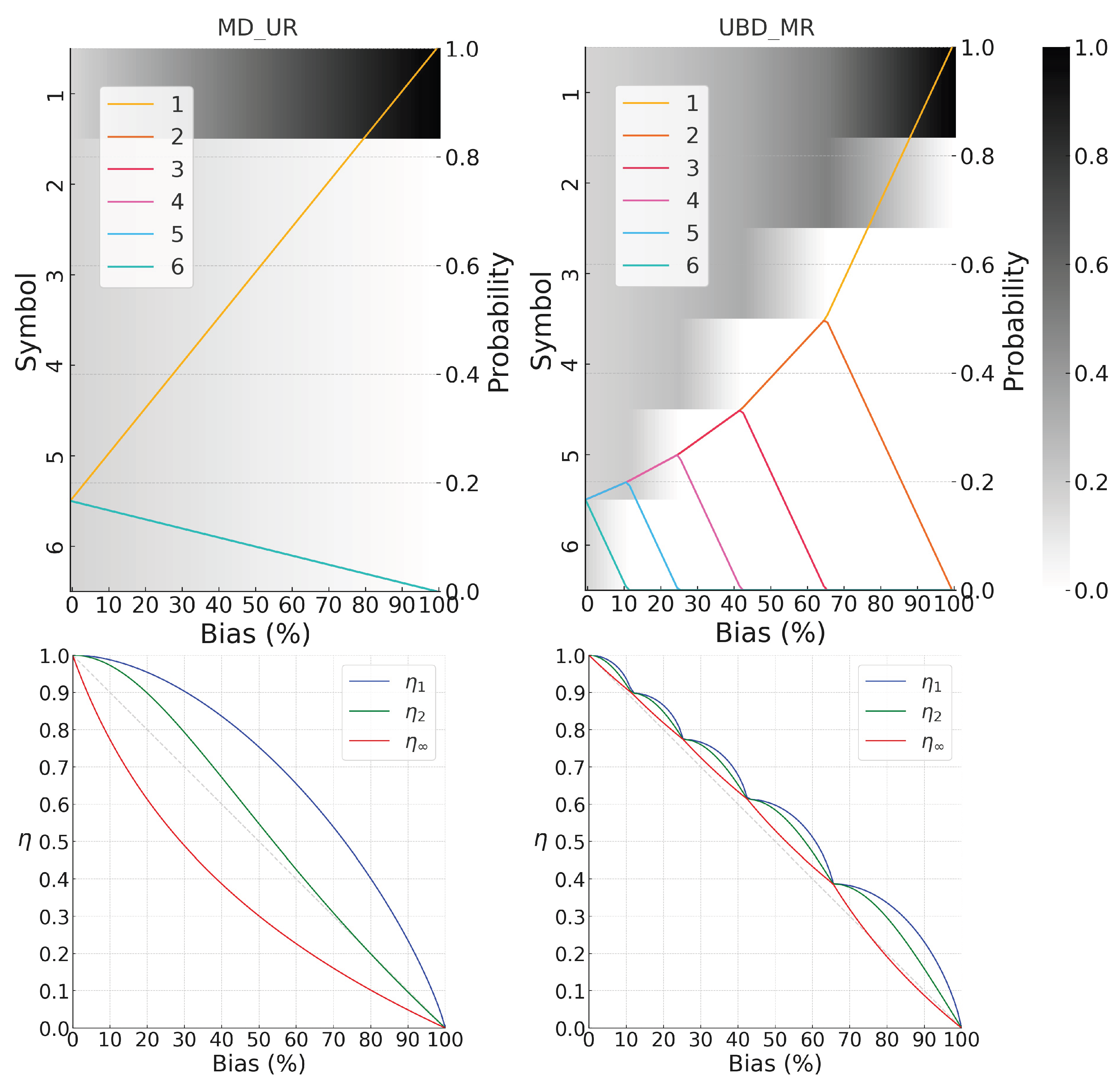
Figure 2.
Localization of the possible state points (in terms of entropies) of any theoretical probability distribution associated with a stochastic process with and arbitrary dimension d. In light blue, the region of state points ; in orange, the region of state points . The regions are bounded by the state points generated by the MD_UR and UBD_MR families of probability distributions.
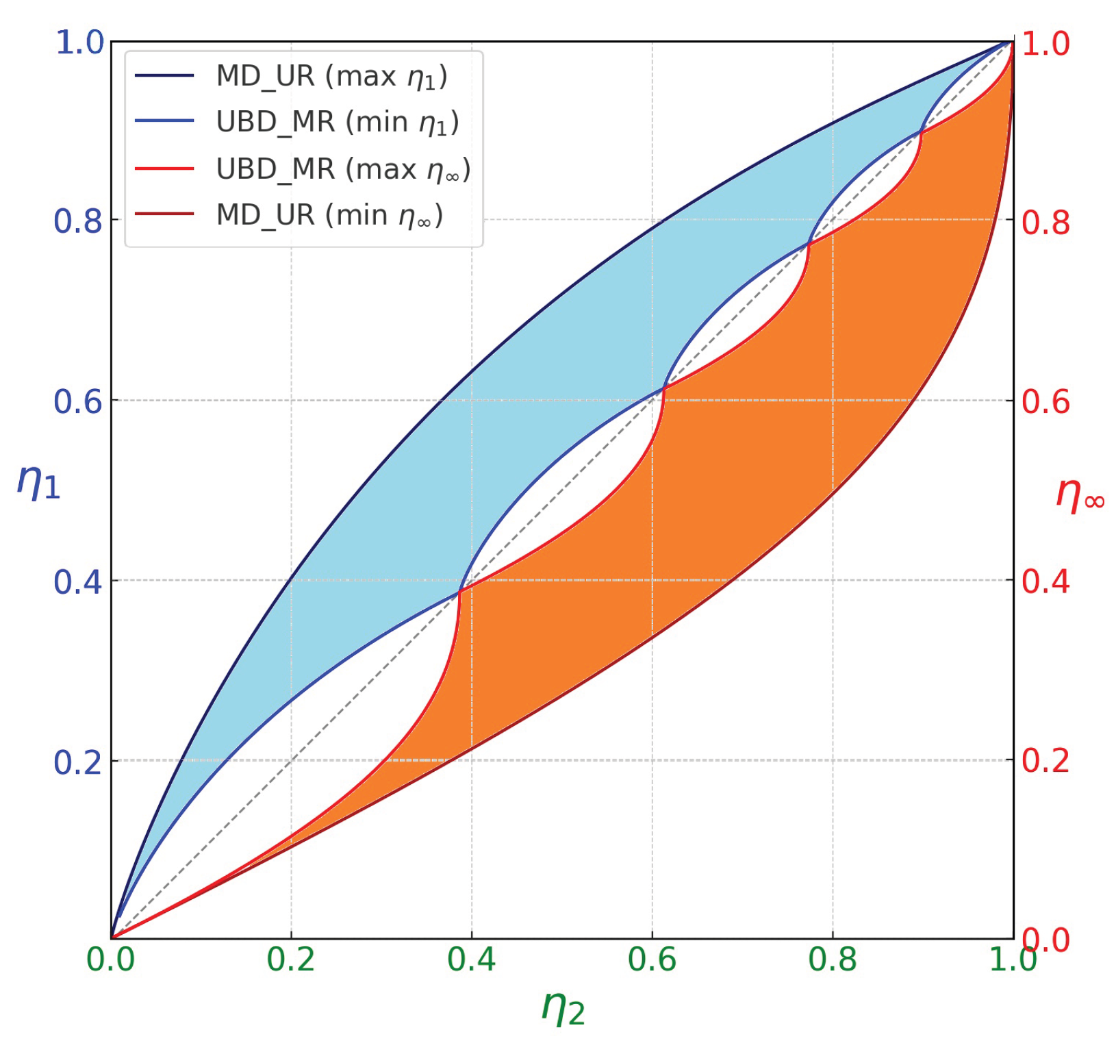
Figure 3.
Example of two distinct probability distributions, and , both defined over an alphabet of size , that share the same specific Shannon entropy () but differ in specific collision entropy (). A comparison based solely on Shannon entropy fails to distinguish them. However, their differing structures become evident when analyzing the entropy pairs and , which occupy distinct positions in the entropy plane.
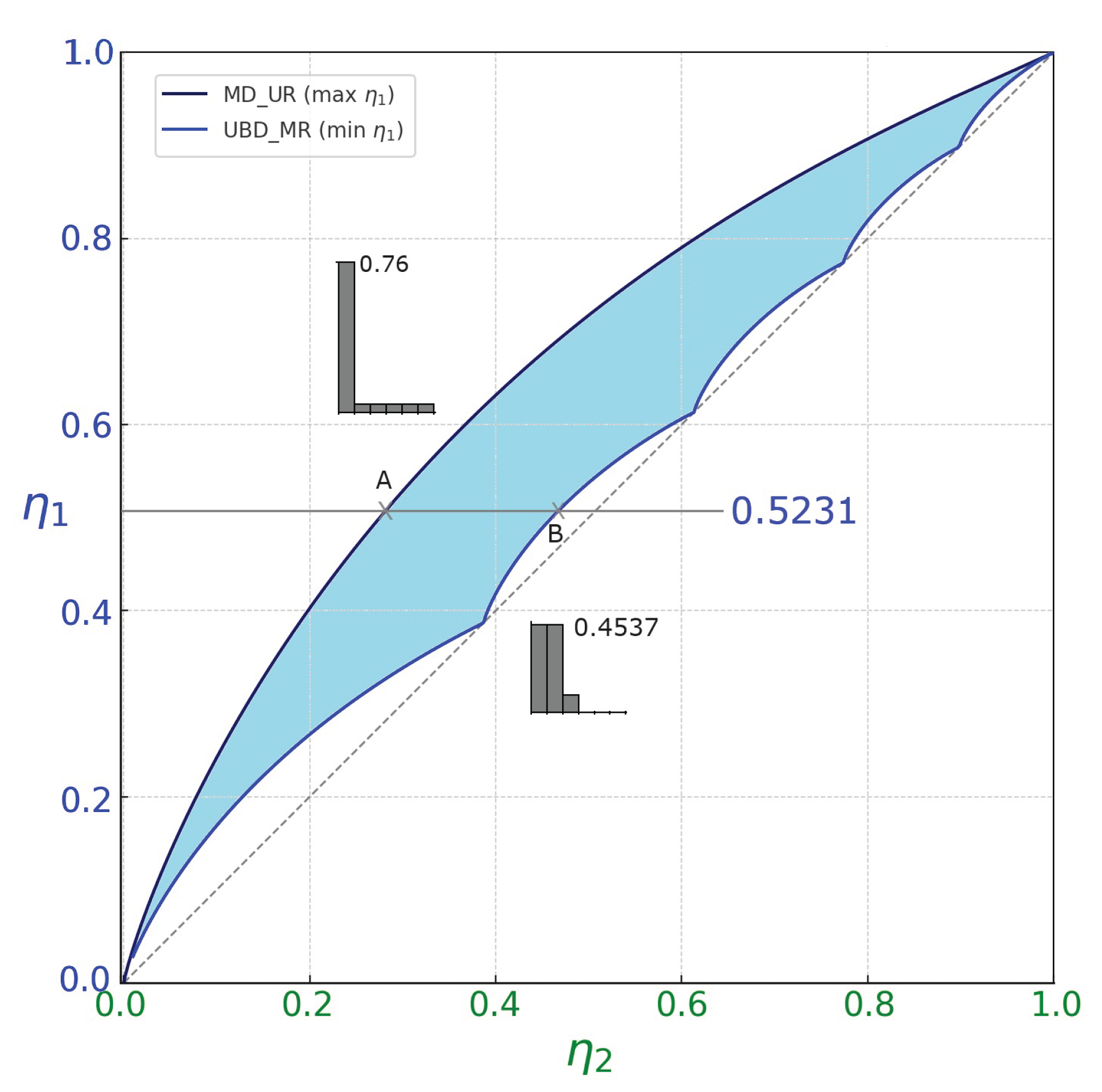
Figure 4.
Apparent vs. actual specific entropies for the MD_UR family of probability distributions.
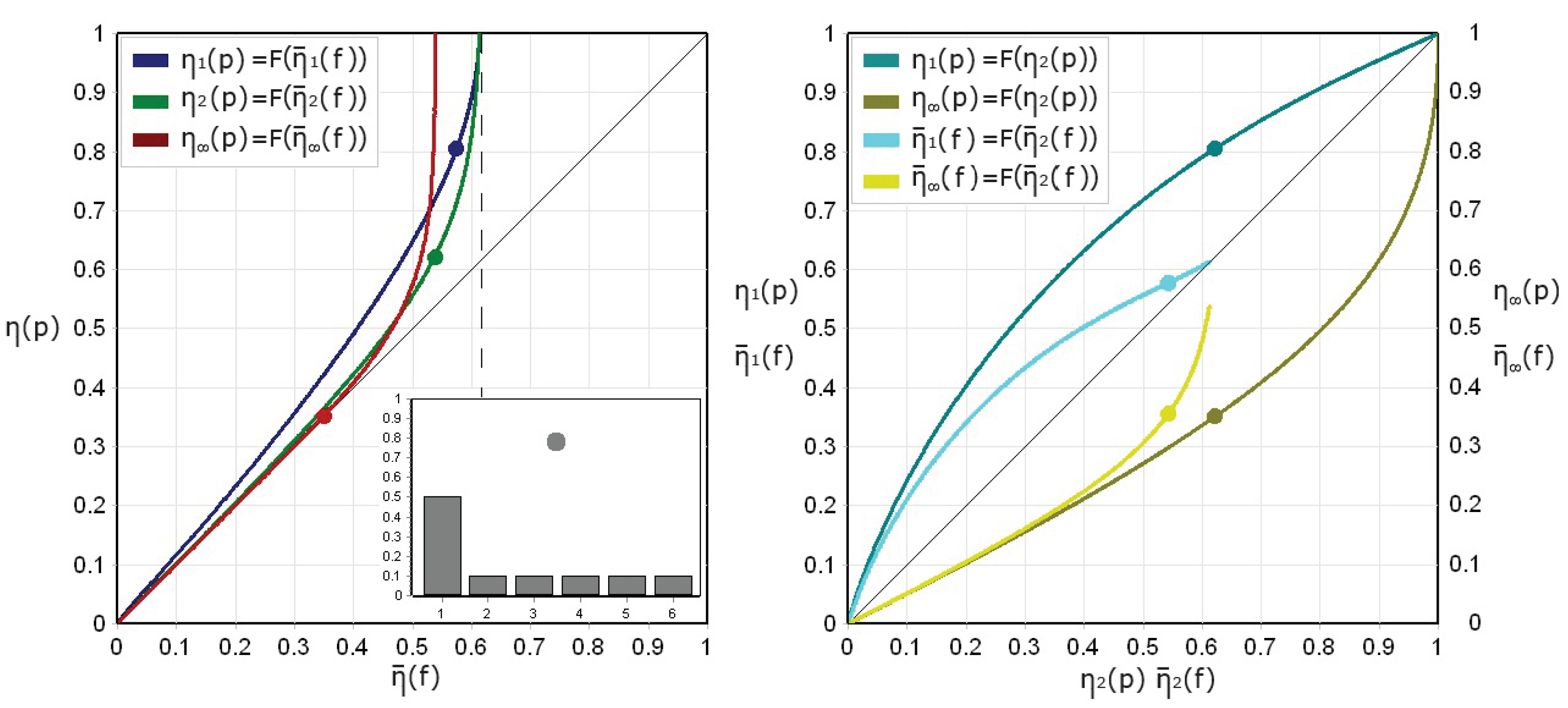
Figure 5.
Apparent vs. actual specific entropies for the UBD_MR family of probability distributions.
Figure 5.
Apparent vs. actual specific entropies for the UBD_MR family of probability distributions.
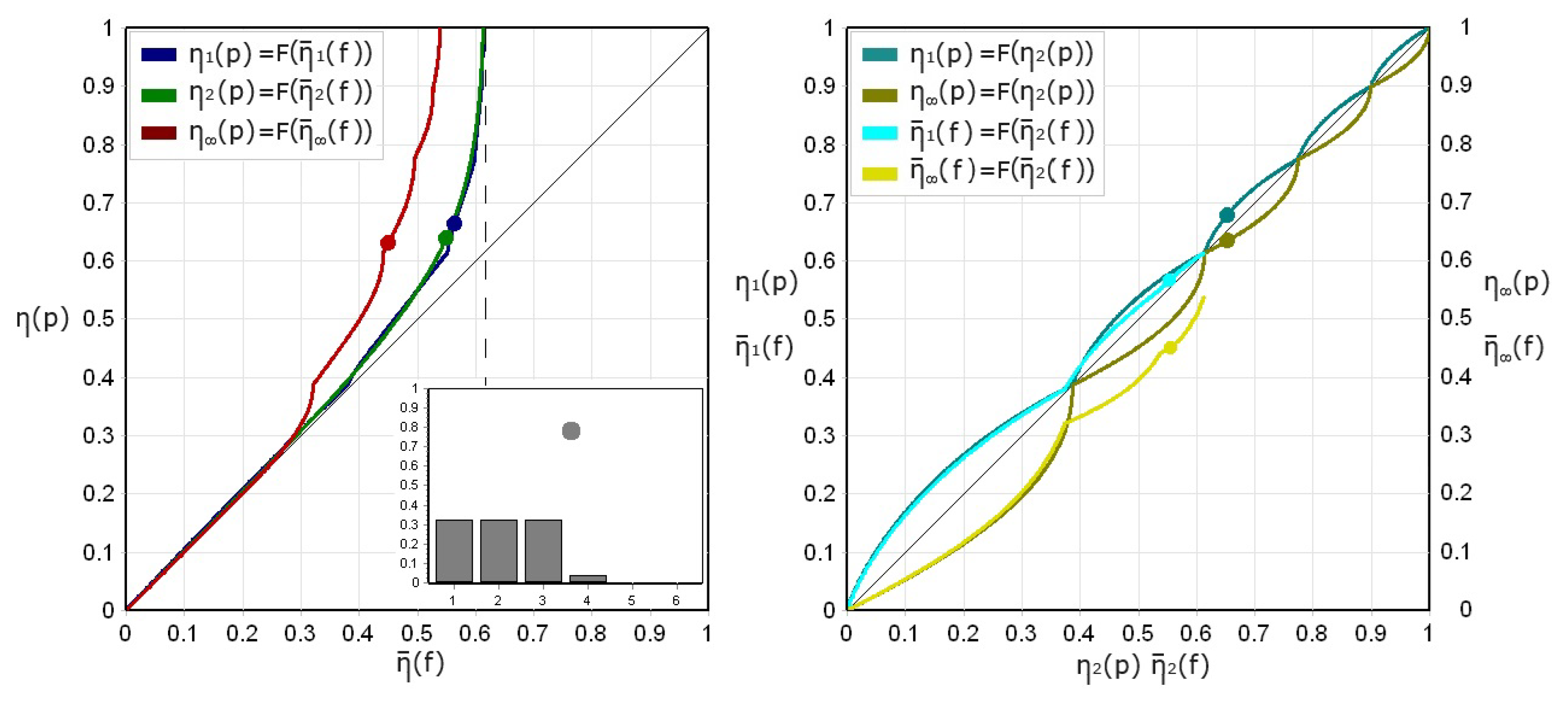
Figure 6.
Left column: Relationship between apparent specific entropies and true specific entropies for processes generated by distributions bounded by the MD_UR and UBD_MR families. Results from previous figures (Figure 4 and Figure 5) are reorganized here by entropy type: in blue, in green, and in red. Right column: Effect of the transformation described by Equation (33).
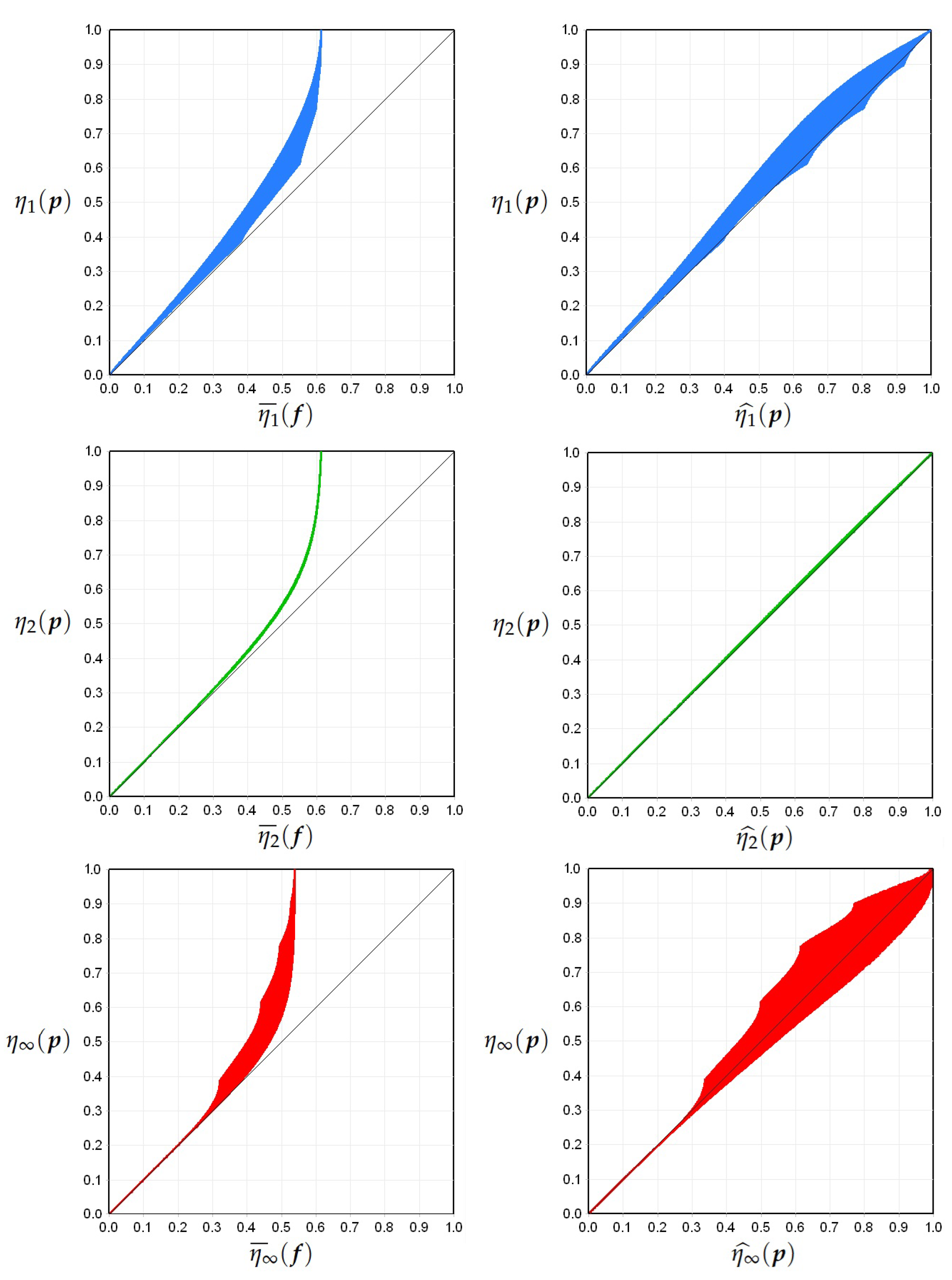
Figure 7.
Left: representation of the regions associated to the relative frequency distributions generated using realizations with 254 samples and whose data are inserted in a 5-dimensional sample space (the same parameters of the previous figures): in blue and in red. The observed contraction relative to the theoretical bounds with respect to the theoretical bounds arises because of the limited amount of data. Right: effect of the affine transformation on the reduced regions: the stretched regions and touch the maximum entropy vertex in , but yet cannot completely overlap the original theoretical region.
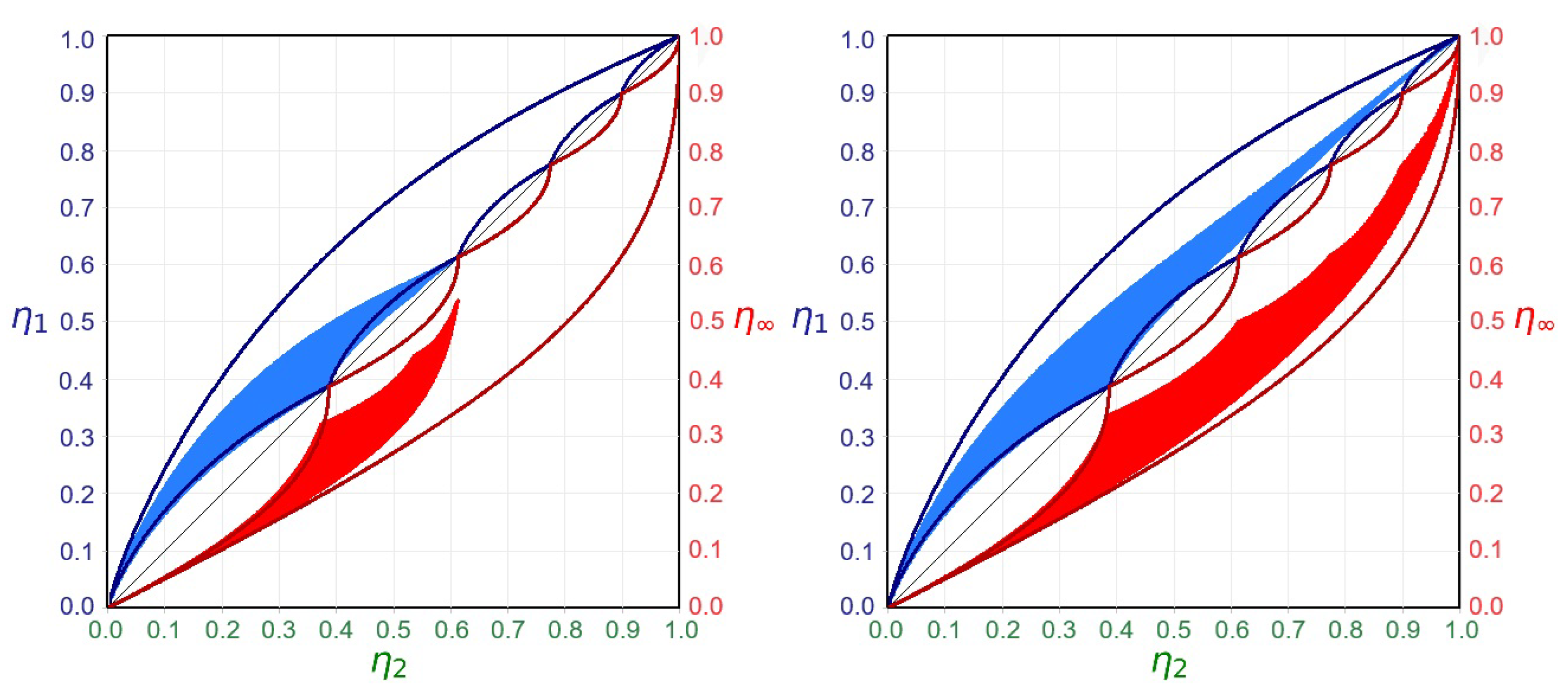
Figure 8.
Final diagram of the example described in § Section 3.7. Specifically: (a) the light blue and light red regions represent the stretched domains obtained by applying the affine transformation to the compressed regions corresponding to empirical relative frequency distributions; (b) point T: the entropic state of the original probability distribution of the process; (c) point S: the average entropic state computed from 1,000 empirical relative frequency distributions; (d) point E: the center of gravity of the points resulting from the affine transformation applied to the Rényi means of the data.
Disclaimer/Publisher’s Note: The statements, opinions and data contained in all publications are solely those of the individual author(s) and contributor(s) and not of MDPI and/or the editor(s). MDPI and/or the editor(s) disclaim responsibility for any injury to people or property resulting from any ideas, methods, instructions or products referred to in the content. |
© 2025 by the authors. Licensee MDPI, Basel, Switzerland. This article is an open access article distributed under the terms and conditions of the Creative Commons Attribution (CC BY) license (http://creativecommons.org/licenses/by/4.0/).
Copyright: This open access article is published under a Creative Commons CC BY 4.0 license, which permit the free download, distribution, and reuse, provided that the author and preprint are cited in any reuse.


