
Submitted:
07 November 2024
Posted:
11 November 2024
You are already at the latest version
Abstract
During switching and impulse actions in electrical systems, transient electromagnetic processes occur. This leads to dangerous current surges and overvoltages, which pose a significant danger to the equipment, and also reduce the reliability of the protection used. The simulation time of such processes is significantly increased for complex electromagnetic devices. Modern requests from design engineers require an increasing the speed of real-time simulation. The use of spectral methods will significantly speed up the calculation of transient processes and ensure high accuracy. At present, we are not aware of any publications showing the use of spectral methods for calculating transient processes in electromagnetic devices containing ferromagnetic cores. The purpose of the work is to develop a highly efficient method for calculating electromagnetic transients in magnetoelectric circuits for replacing a coil on a ferromagnetic core connected to a voltage source. The method is based on the use of nonlinear magnetoelectric schemes for replacing electromagnetic devices and a spectral method for representing solution functions by orthogonal polynomials. At the same time, a schematic model for the use of the spectral method was developed. Results. Methods for calculating transient processes in magnetoelectric circuits based on approximation of solution functions by series of algebraic polynomials, as well as Chebyshev, Hermite, and Legendre polynomials have been developed and investigated. The proposed method has made it possible to transform integro-differential equations of state describing transient processes in magnetoelectric circuits into linear algebraic equations for depicting solution functions. The developed schemat-ic model simplifies the use of the calculation method. Images of the true functions of electric and magnetic currents are interpreted as direct currents in the proposed substitution scheme. Based on the described methods, a computer program has been developed to simulate transient processes in a magnetoelectric circuit. The comparison of methods made it possible to choose the optimal type of polynomial. The advantage of the presented method over other known methods is the reduction in the simulation time of electromagnetic transients (for the examples considered, more than 12 times faster than in the implicit Euler calculation) while ensuring the same accuracy. The calculation of the process in the circuit over a long time interval showed a decrease and stabilization of errors, which indicates the prospects of using the proposed methods for the calculation of more complex electromagnetic devices (for example, transformers).
Keywords:
1. Introduction
2. Basics of Transformations for Obtaining Magnetoelectric Equivalent Circuits
- -
- equivalent magneto-electric circuits of power transformers are very complicated;
- -
- transients in these transformers have very long time, and with rapidly changing components of processes;
- -
- the time of simulating transients is significant, which is undesirable.
- -
- To speed up the simulating process, it is proposed to use orthogonal polynomials.
3. Basics of Using Orthogonal Polynomials to Integrate Differential Equations
Generation of Matrix Equations
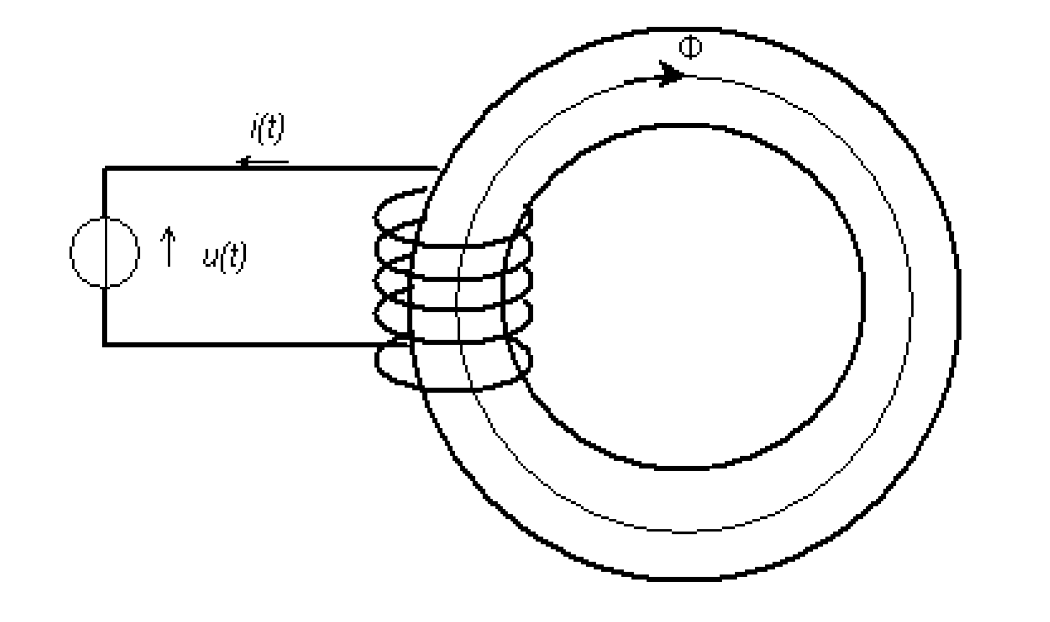
4. Using Orthogonal Polynomials to Calculate Transients in a Ferromagnetic Core Coil
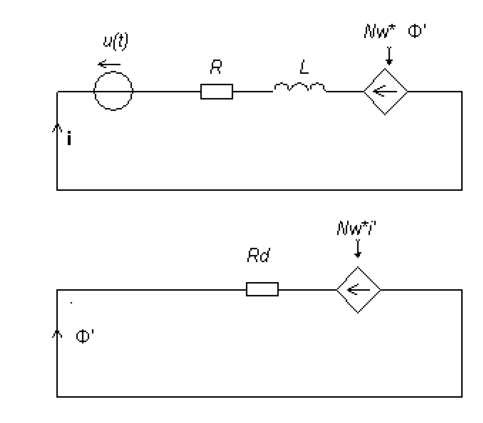
4.1. General Equations

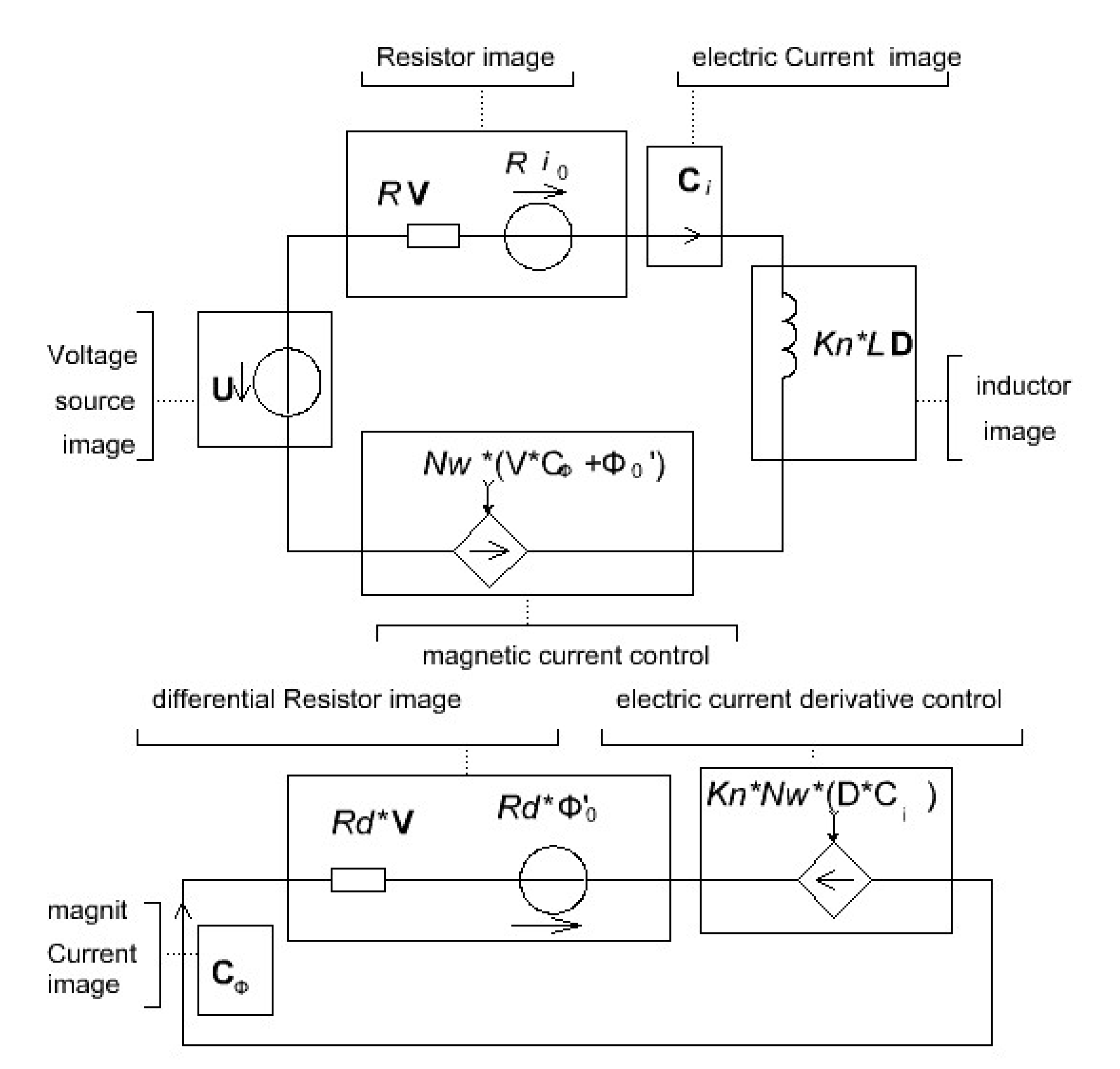
4.2. Schematic Interpretation of the Method of Numerical Calculation of Transients in Magnetoelectric Circuits
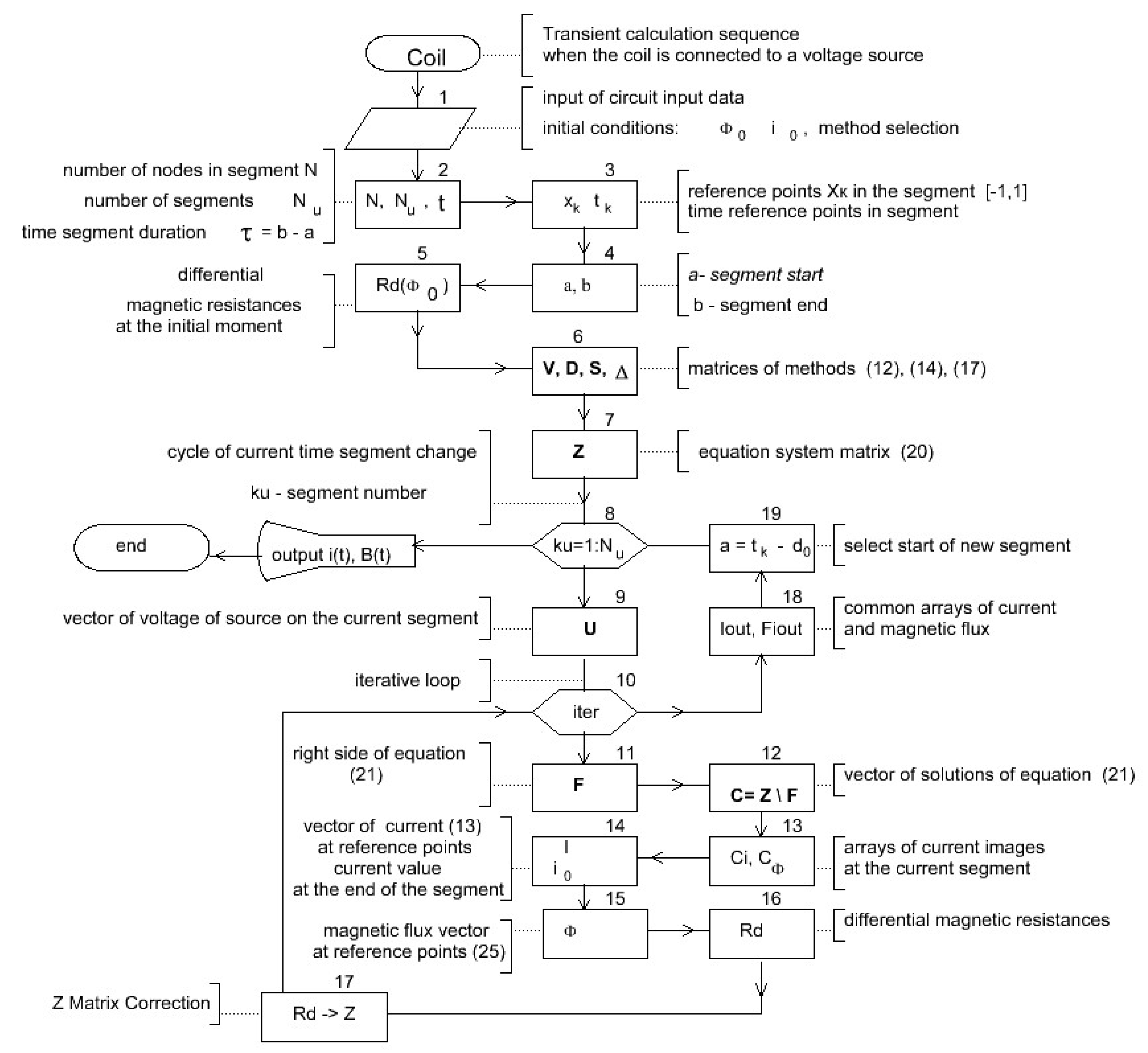
4.3. Calculation Algorithm, Programs and Simulation Results
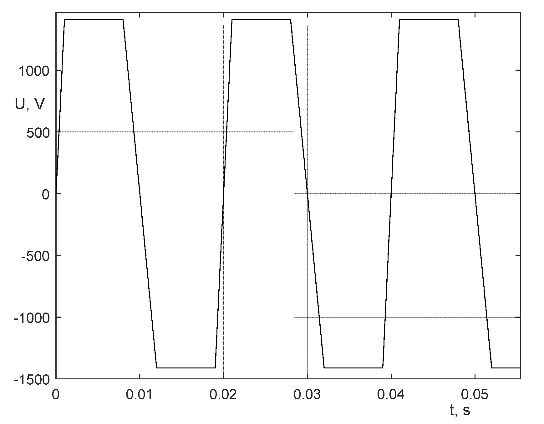
- Input of initial data (start time tbegin and end time of simulation tend, time segment dimension τ, electric circuit parameters R, L, e(t), core coil parameters S, l, magnetization curve B (H), initial conditions Φ0, i0) is performed. The orthogonal polynomial type is selected.
- It is set: the number N of reference points on a segment without a zero point (7 points are recommended for each segment), the length of the time segment, the segments number Nu is calculated over the entire time investigated interval.
- To calculate the coefficients of orthogonal polynomials the positions of the reference points xk on interval [-1, 1] of one segment (the position of the reference points on all segments is the same) are set. In the paper [10] it is shown that the reference points can be set uniformly, and also thickened to the ends of the segment or to the middle of the segment.
- The segment is specified in the interval [a, b] on the timeline, where a and b are the start and end times of the segment, with τ=b-a. Corresponding to the locations of the reference points xk on [-1, 1] the reference points tk on the time interval [a, b] are calculated using the formula
- 5.
- The initial differential magnetic resistance of the Rd0 of magnetic branch is calculated from the initial value of the magnetic flux Φ0 of the ferromagnetic.
- 6.
- The values of matrices V, D, S, Δ for the left part of the Equation (21) are calculated.
- 7.
- It is filled in matrix Z, in which the initial differential magnetic resistance Rd0 is used.
- 8.
- Current calculations for each segment on time interval [a, b] are cyclically performed (items 8-18). Segment numbers are cyclically changed from 1 up to Nu. When the ku cycle parameter changes, it is performed the following acts :
- 9.
- The values of the source voltage vector U at all points of the segment are calculated.
- 10.
- Iterative cycle (items 10-16) of current calculation for reference points of the current segment is performed. The iterative cycle is necessary to clarify the value of the differential magnetic resistance Rd, since this value depends on the value of the magnetic flux.
- 11.
- The matrix Z containing the value of the magnetic resistance Rd is clarified. The vector of the right parts F of the system (23) is calculated.
- 12.
- System of algebraic equations is solved and vector of polynomial coefficients C=Z-1·F is determined.
- 13.
- The vectors of polynomial coefficients Ci , CΦ for each current are distinguished.
- 14.
- Vectors of values of all currents (including magnetic currents) are calculated based on values of vectors Ci, CΦ according to (13).
- 15.
- A vector of magnetic flux values at reference points is calculated using the formula (25) for calculation of integral.
- 16.
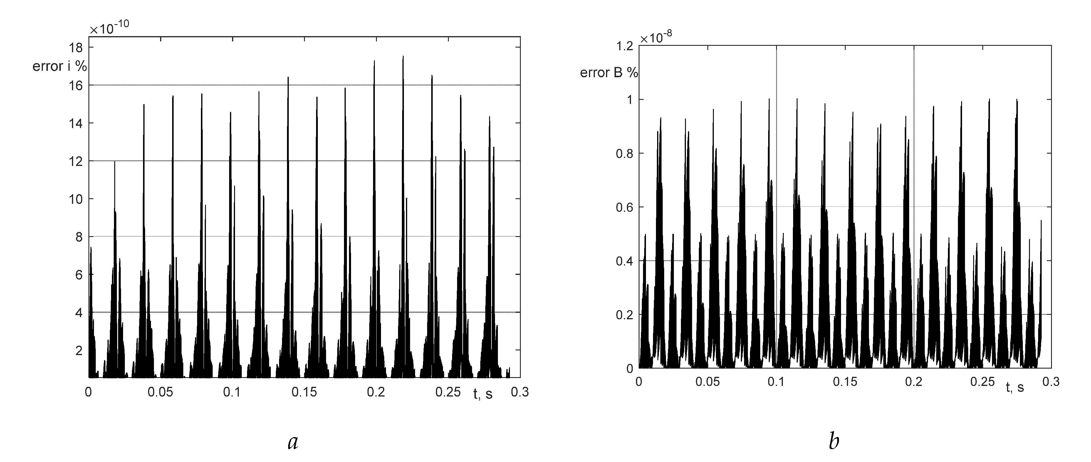
- The differential magnetic resistance Rd of the branch is calculated from the values of the magnetic flux according to the magnetization curve of the ferromagnetic, using the function of approximation by splines of the magnetization curve. The end condition of the iteration loop is checked. The iteration cycle (items 10-16) ends if the values of magnetic resistance of adjacent iteration cycles do not exceed the specified error, otherwise we return to item 10.
- 17.
- The last current and magnetic flux values on the current segment will become the initial current and magnetic flux values for the next segment when the iterative cycle is terminated.
- 18.
- Current and magnetic flux values are stored in arrays for output at the end of calculation.
- 19.
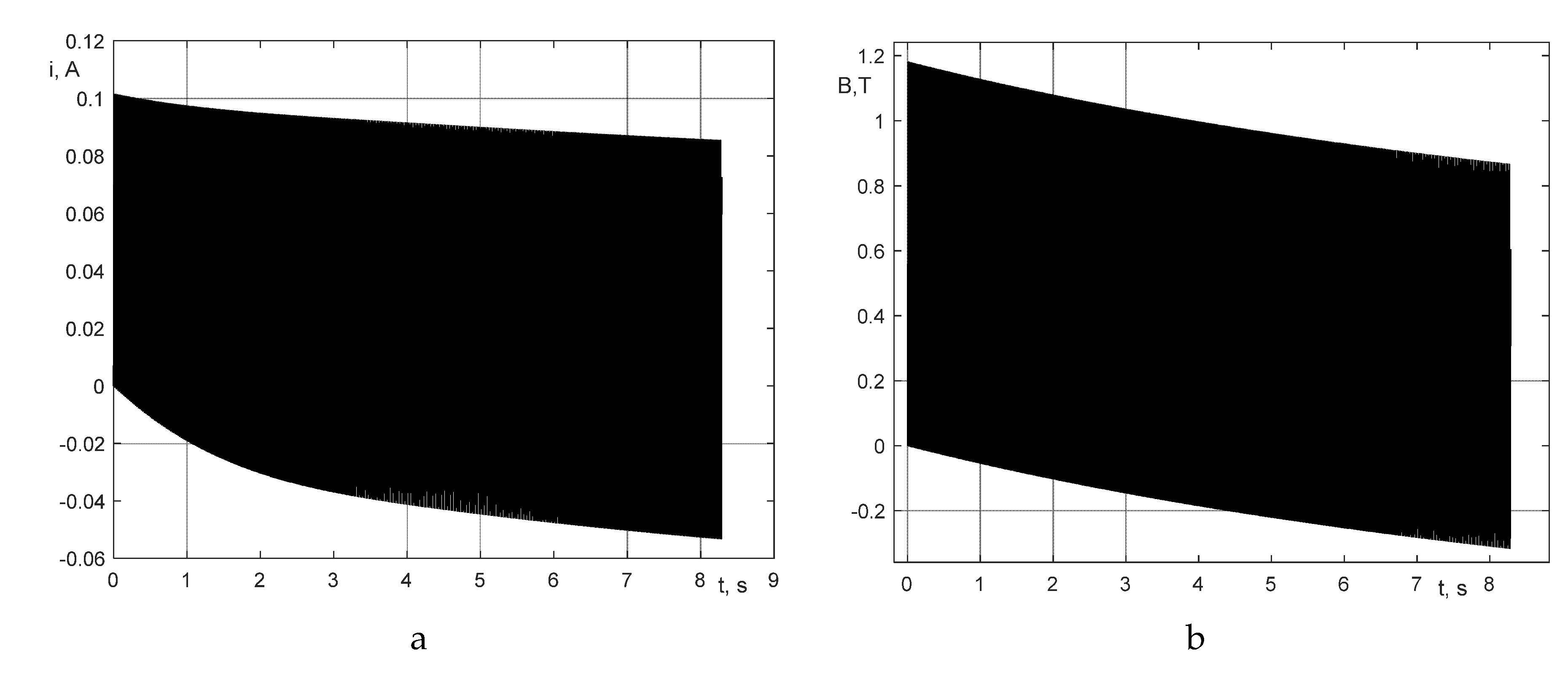
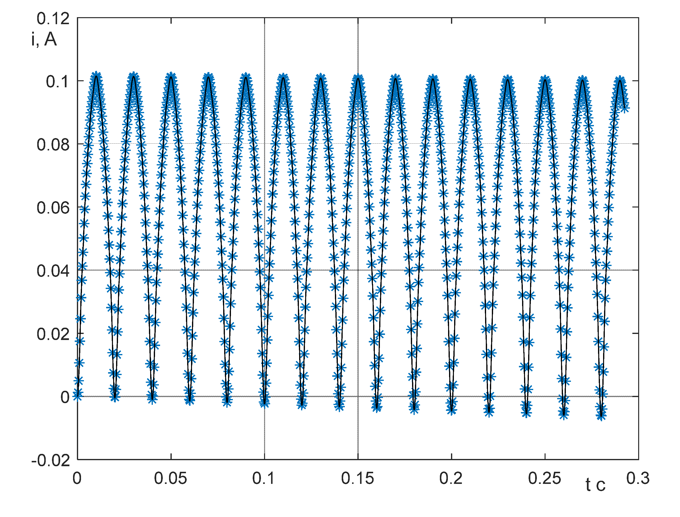
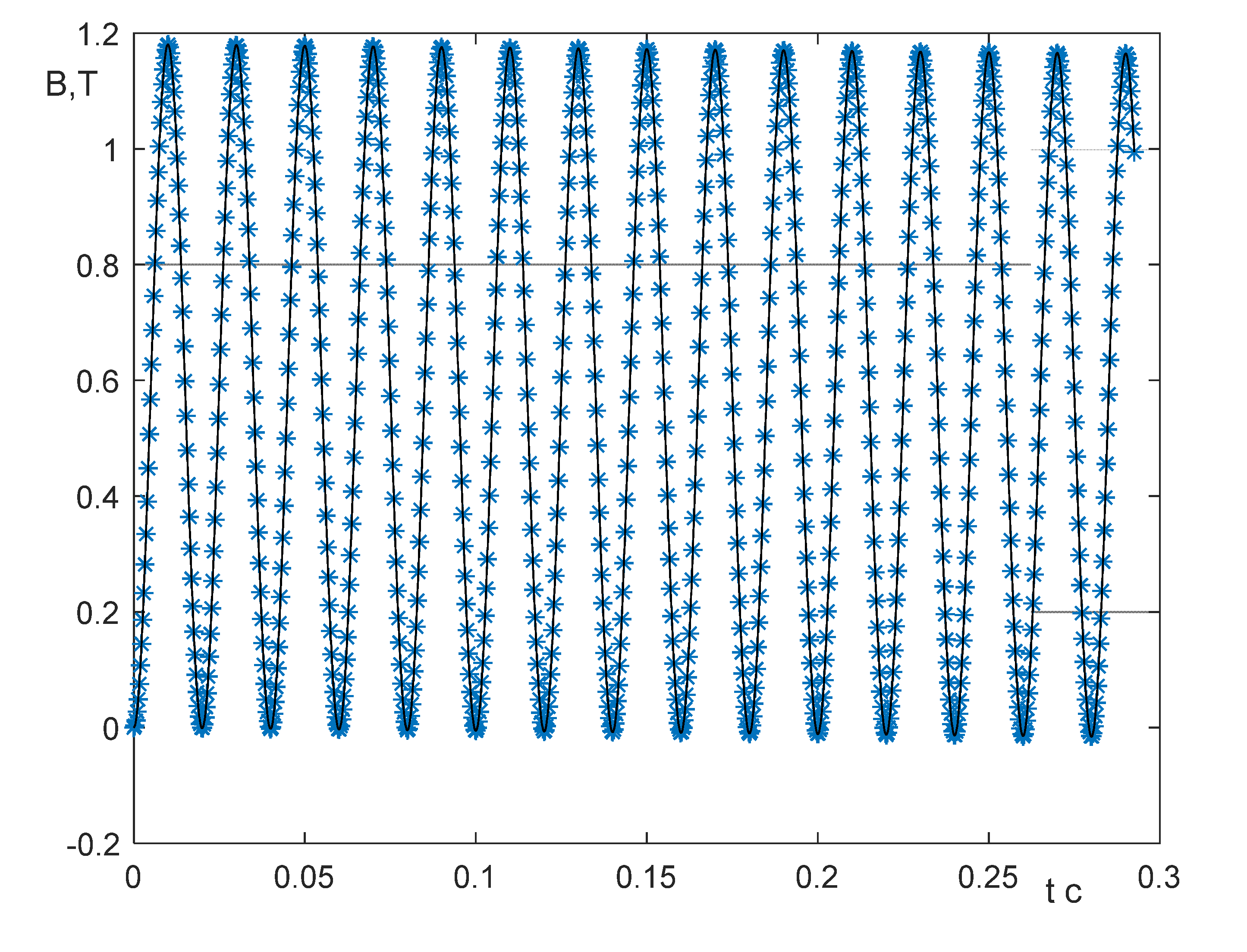
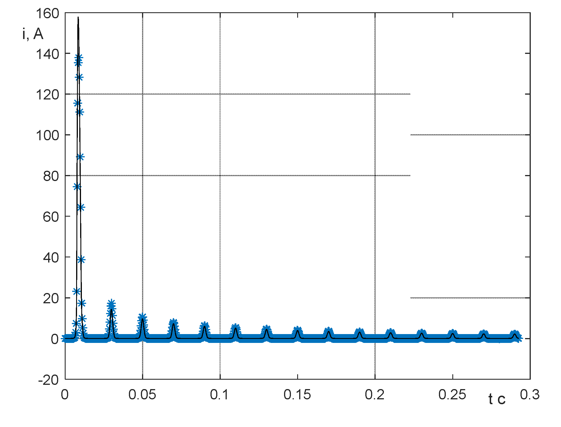
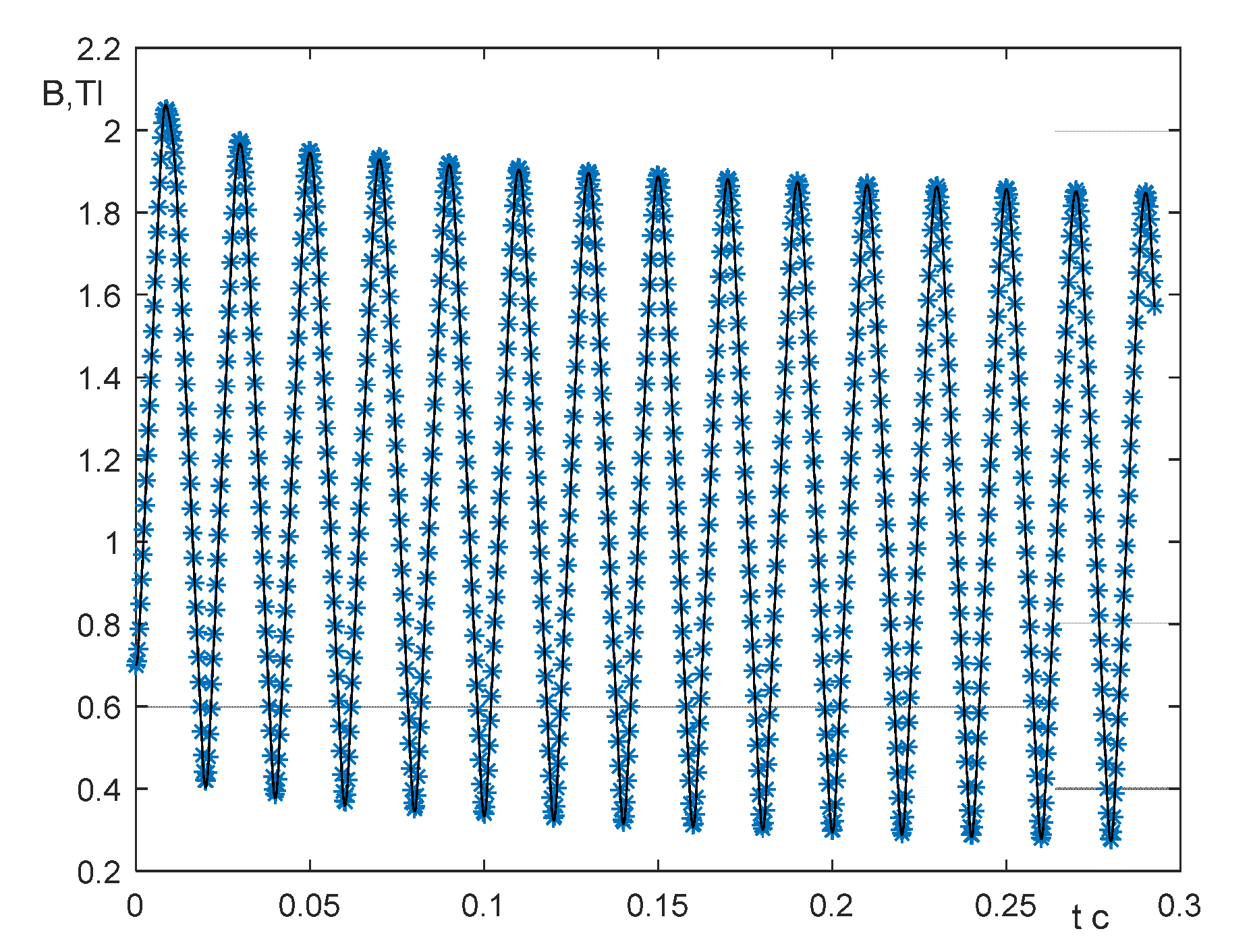
- The graphs of the transient in the time area are generated.
5. Discussion
6. Conclusions
References
- Shakirov M.A. Analysis of non-uniformity of distribution of magnetic loadings and losses in transformers based on magnetoelectric equivalent circuits. Elektrichestvo [Electricity]. 2005.11. 15-27. (In Russian).
- Lipman A.A. “Electric” and “magnetic” circuits of the electromagnetic circuit. Elektrichestvo [Electricity]. 1974, 7, pp. 65-68. (In Russian).
- J.C. Butcher (2015) Runge–Kutta Methods for Ordinary Differential Equations. © Springer International Publishing Switzerland 2015 M. Al-Baali et al. (eds.), Numerical Analysis and Optimization, Springer Proceedings in Mathematics & Statistics 134. [CrossRef]
- Epperson, James F., (2013). An introduction to numerical methods and analysis / James F. Epperson, Mathematical Reviews. — Second edition. pages cm Includes bibliographical references and index. ISBN 978-1-118-36759-9 (hardback).
- Carl de Boor. A Practical Guide to Splines. Textbook © 1978. – 304 с. https://link.springer9780.
- Tykhovod S. M. Computer modulation system of dynamic processes in nonlinear magnetoelectric circuits. Tekhnchna elektrodinamka. [Technical electrodynamics]. 2008. 3, 16-23. (In Russian).
- Epperson, James F., (2013). An introduction to numerical methods and analysis / James F. Epperson, Mathematical Reviews. — Second edition. pages cm Includes bibliographical references and index. ISBN 978-1-118-36759-9 (hardback).
- John, P. Boyd (2000) Chebyshev and Fourier Spectral Methods. University of Michigan Ann Arbor, Michigan 48109-2143 email: jpboyd@engin.umich.edu http://www-personal.engin.umich.edu/∼jpboyd/ DOVER Publications, Inc. 31 East 2nd Street Mineola, New York 11501 594 с.
- Lloyd, N. Trefethen (2000) Spectral Methods in MATLAB. SIAM, - 181 с https://riin.info/compress-pdf.html.
- Sergii Tykhovod and Ihor Orlovskyi Development and Research of Method in the Calculation of Transients in Electrical Circuits Based on Polynomials. Energies 2022, 15, 8550. 1–17. [CrossRef]
- Bateman, H. , Erdelyi A.(1955) Higher transcendental functions. Volume 2. New York, Toronto, London, 296 p.
- Ansys, engineering Simulation Software. https://www.ansys.com/.
- COMSOL - Software for Multiphysics Simulation. https://www.comsol.com/.
- Tykhovod S. M. Computer analysis of magnetic fields by the method of contour fluxes. Elektrotekhnka ta elektroenergetika. [Electrical engineering & power engineering]. 2002. 2. 49-52.
- MathWorks - Maker of MATLAB and Simulink. https://www.mathworks.
- Program for calculation of transient in the inductance coil by spectral method. - [Electronic resource]. - access mode: https://drive.google.com/file/d/1LgildZrro5FuHvvEBxaexBtnS38rwqJv/view?
- Program for calculating the transient in the inductance coil by the Euler method. - [Electronic resource]. - access mode: https://drive.google.com/file/d/1zJcrYYZstZEHuWnQqySdHXUW3ul_LW2V/view?
- Program for calculation of transient in the inductance coil by spectral method (trapezoidal voltage). - [Electronic resource]. - access mode: https://drive.google.com/file/d/1M76sBYLmGe9SgxCuTJm8FFy_FOurg2D1/view?
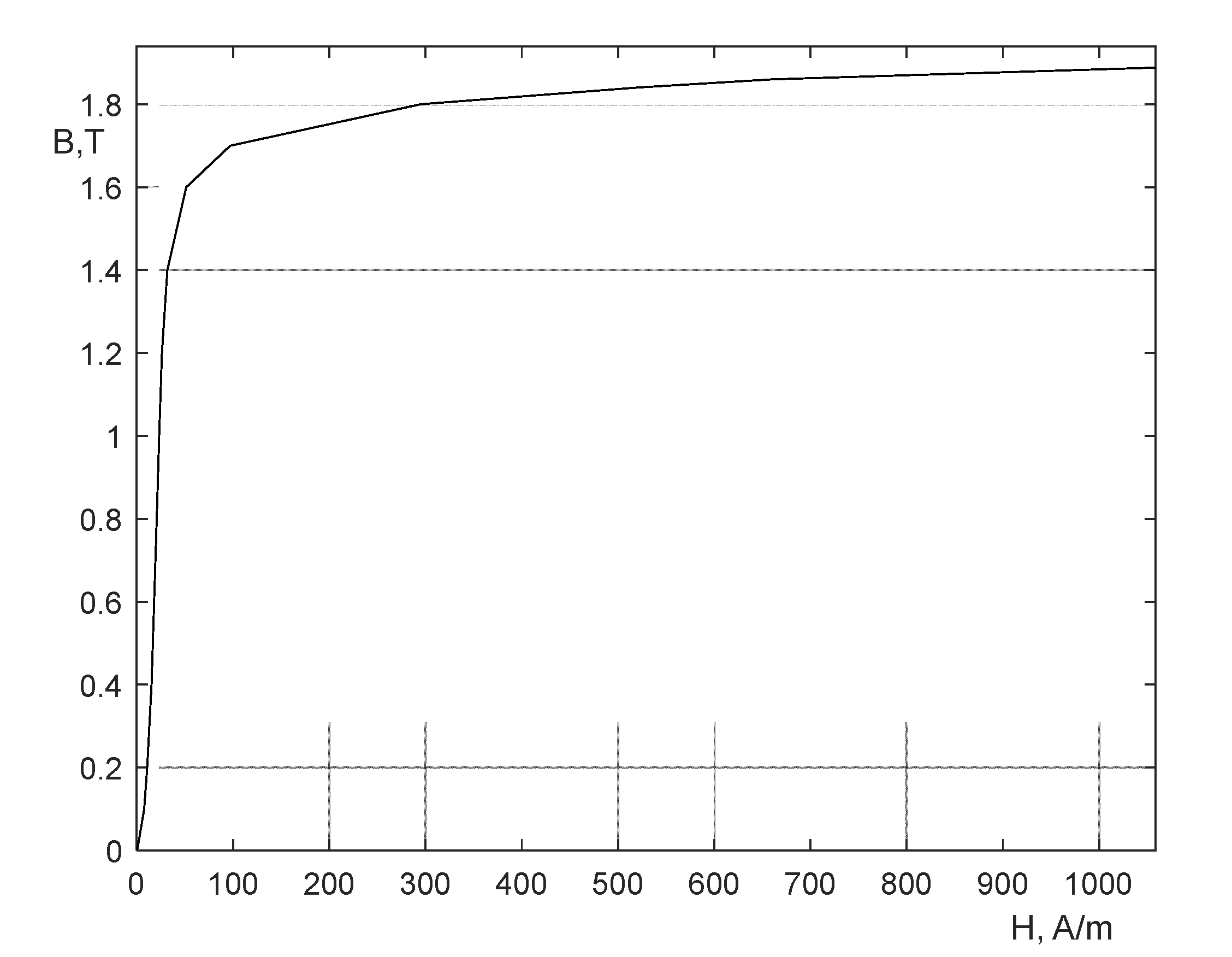

| H (A/m) | 0 | 1 | 7,58 | 10,8 | 15,2 | 20,8 | 23,2 | 26,2 | 31,9 | 51,4 | 97,3 | 520,7 | 1218 | 1,25*105 |
| B (T) | 0 | 0,0096 | 0,1 | 0,2 | 0,4 | 0,8 | 1,0 | 1,2 | 1,4 | 1,6 | 1,7 | 1,8, | 1,84 | 2 |
| ID | Δ % | Algebraic polynomials |
Chebyshev polynomials |
Legendre polynomials |
Hermite polynomials |
||||||||
| B0,T | zeros | max | uniform | zeros | max | uniform | zeros | max | uniform | zeros | max | uniform | |
| 0 | Δi | 0.0036 | 0.0036 | 0.0035 | 0.0036 | 0.0022 | 0.0033 | 0.0036 | 0.0309 | 0.0789 | 0.0480 | 0.0414 | 0.0397 |
| ΔB | 0.0034 | 0.00346 | 0.00347 | 0.0034 | 0.0035 | 0.0035 | 0.0034 | 0.0039 | 0.0049 | 0.0035 | 0.0034 | 0.0035 | |
| 0,7 | Δi | 0.1018 | 0.1032 | 0.1087 | 0.1018 | 0.1031 | 0.1085 | 0.1018 | 0.1209 | 0.1964 | 0.111 | 0.1117 | 0.1159 |
| ΔB | 0.0092 | 0.0093 | 0.0092 | 0.0092 | 0.0093 | 0.0092 | 0.0092 | 0.0085 | 0.0203 | 0.0099 | 0.0093 | 0.0092 | |
| Δ % | Algebraic polynomials |
Chebyshev polynomials |
Legendre polynomials |
Hermite polynomials |
||||||||
| zeros | max | uniform | zeros | max | uniform | zeros | max | uniform | zeros | max | uniform | |
| Δi | 1.0325 | 1.0458 | 1.1012 | 1.0324 | 1.0457 | 1.1012 | 1.0323 | 1.0451 | 1.1007 | 1.0553 | 1.0539 | 1.583 |
| ΔB | 0.280 | 0.2841 | 0.294 | 0.2807 | 0.284 | 0.2944 | 0.2792 | 0.2436 | 0.29632 | 1.0371 | 0.7169 | 2.962 |
Disclaimer/Publisher’s Note: The statements, opinions and data contained in all publications are solely those of the individual author(s) and contributor(s) and not of MDPI and/or the editor(s). MDPI and/or the editor(s) disclaim responsibility for any injury to people or property resulting from any ideas, methods, instructions or products referred to in the content. |
© 2024 by the authors. Licensee MDPI, Basel, Switzerland. This article is an open access article distributed under the terms and conditions of the Creative Commons Attribution (CC BY) license (http://creativecommons.org/licenses/by/4.0/).


