
Submitted:
07 November 2024
Posted:
08 November 2024
You are already at the latest version
Abstract
The connectivity reliability of public transport depends on a number of factors, including public transport routes, the connections between them, their frequency, their availability, and the availability of public transport and infrastructure. A shortest path algorithm is used to find up to "k" paths connecting each Origin-Destination pair in space-time, taking into account the schedules and a constraint on the maximum tolerable waiting time. For each path, four reliability indicators are proposed, as well as an approachability indicator, related to the level of transport supply. Thanks to two sets of equations, these indicators are also computed on the origin-destination and network levels. This enables fleet managers to evaluate and compare strategies for improving the connectivity reliability and the transport supply, such as increasing the number of public transport routes, reducing route length or increasing frequency. From an application on the bus network of a city in Brittany in France, we show how to understand and use these indicators.
Keywords:
Reliability
; Dynamic Connectivity
; Public Transport Network
; “k” shortest paths algorithm
; {time x space}
; Assessment
1. Introduction
In the following, we will talk more specifically about buses, but the equations and reasoning apply to all types of public transport. For users, the reliability of public transport and the level of transport supply are essential. Fleet managers evaluate various reliability factors and the transport supply. A number of studies (Section 2, State of the art) have analyzed many dimensions of reliability; generally, only the shortest path linking an origin to a destination is considered, although all the paths connecting origins to destinations contribute to reliability. Our contribution (summarized in Section 3) consists in characterizing the contribution to reliability of “k” paths for each Origin-Destination (OD) pair; these paths are found, at every departure time, thanks to a “k” shortest paths algorithm [1]; this algorithm is implemented in the space-time, taking into account timetables and a limit on the maximum tolerable waiting time (Appendix A). We provide fleet managers with a set of indicators (Section 4), useful for identifying the most disadvantaged Origin-Destination pairs, and on the basis of which service improvement projects can be compared. In Section 5, equations provide the contribution of the various paths to reliability and unreliability (defined here as one minus reliability). An application (Section 6) to the bus network of a city in Brittany shows how to understand and use these indicators; the impact of node closure is shown in Appendix C.
2. State of the Art
Wakabayashi and Iida defined reliability as ‘‘the probability of a device performing its purpose adequately for the period intended under the operating conditions encountered’’ [2] – applied to transport networks, it is, according to Nicholson, “the probability that a trip can be successfully finished within a specified time interval”[3]. Reliability is generally used to describe the stability, certainty, and predictability of travel conditions [4].
Understanding the causes and consequences of unreliability, assessing reliability, possibly model it, proposing its enhancement, are useful for developing networks and allocating capacity, for the appraisal of transportation projects, for passenger route choice, as well as for diagnosing critical locations in transportation infrastructure.
In a public transportation network, the main causes of unreliability are, according to Mahdavi et al. [5], failure on physical infrastructure or on fleet service and uncertainty on travel demand and travel time.
2.1. Failure in the Connection Between Origin and Destinations
Bell and Iida defined connectivity reliability as the probability of having a connection between a pair of nodes when one or more links are removed [6]. Similar definitions are proposed in [7,8,9]. Kim gave flow reliability, and topological reliability indicators, based on the supply at the OD level and the bus route level [10].
Vulnerability, the opposite of reliability, is addressed in [11,12,13,14,15,16]; Cats and Jenelius established a vulnerability curve showing the relationship between network performance and the degradation of route or link capacities [17]; for a rail network, Liu [18,19] determined the economic value of reserve capacity and determined its impact for enhancing reliability and robustness: the disturbances cause train delays as well as cancellations. Taylor and D’Este developed a method for diagnosing critical points in transportation infrastructure [20].
However, only one path per OD pair is considered, whereas all paths would have to be considered, for determining whether or not the failure of a link or of a public transport vehicle leads to a disconnection of the OD pair.
2.2. Uncertainty on Travel Time or Travel Demand
A trip may not be completed on time due to an increase in travel time. Indicators measuring the variability of travel time distribution define travel time reliability, which intervenes in the overall reliability at (at least) three levels:
- To suggest ways of enhancing overall reliability. Muñoz, after analyzing the sources of irregularity, proposed to regularize headways, thereby improving reliability [24]. Artan and Sahin developed a stochastic model, to be used in the timetable design phase, to prevent the impact of cumulative delays on reliability [25].
- To offer passengers the most reliable routes. Waiting time reliability has an impact on the passenger route choice- this was evaluated by Shelat [26]; Khani developed a stochastic algorithm capable of proposing the most reliable route (in terms of time) [27] - in addition, proposed backup itineraries are proposed by Redmond [28].
Excessive passenger demand may also prevent a trip from being completed in time. To reduce this negative effect, Liu optimized the reserve capacity [19]. A number of works, initially carried out for road networks, could be adapted to public transportation networks: Clark and Walting modeled network travel time reliability based on daily demand variability [29]; Chen [30], and Yang [31] defined capacity reliability as the probability that a network can meet a certain traffic demand at a required level of service, while taking into account drivers’ route choice behavior.
All this argues in favor of introducing a stochastic term into the shortest-path algorithm - we have not yet introduced it in the work presented here.
2.3. Reliability and Accessibility
According to Kim and Song, accessibility refers to the ease with which passengers can make their journeys between the network’s origin and destination stations [32].
Travel time reliability and accessibility are closely related concepts [20]; Bimpou and Ferguson integrated day-to-day travel time reliability into the measurement of accessibility [33].
Connectivity reliability and accessibility are also closely related. Kim and Song combined accessibility and topological reliability in a single indicator [34]. Taylor proposed an approachability index, equal to the ratio between the Euclidean distance between an Origin and a Destination and the actual length of the path connecting Origin and Destination [35]. This indicator, valid for a single path, is here generalized for an OD connected by several paths.
3. Research Contribution
The various paths that exist between an origin and a destination contribute to the transport supply and reliability - we clarify and characterize these contributions here; this should help fleet managers to improve service, and passengers to use the service.
- Relation between the reliability logarithm of a path and its length. The Shannon information of an event, measuring its amount of uncertainty, is the absolute value of the logarithm of its probability [36]. Applied to the event “no failure on the path”, it is the absolute value of the logarithm of the path reliability. It appears to be the product of the path length and the failure rate (which is the opposite of the logarithm of the reliability of a unit-length element). Provided that only one path per OD is considered, this extends to the geometric mean of path reliability for all connected ODs, which is therefore related to the average path length.
- Concept of “OD length”, based on the OD reliability logarithm. When an OD pair is connected by several paths in space or time, the previous relation holds when replacing the path length by an “OD length”, defined so that the product of this length and the failure rate is equal to the absolute value of the OD reliability logarithm. The OD length is less than the shortest path length- the reduction in length quantifies the contribution of alternative paths.
- Independence and equivalence degrees. For each path linking a given OD, the “independence coefficient” quantifies the genuinely new part of the path in relation to previous paths. The coefficient equals 1 when the path is entirely distinct from previous paths and is lower when there are overlaps; the “equivalence degree” of a path, relative to the first (shortest) path, combines its independence degree and its lengthening relative to the shortest path. The sum of the equivalence degrees over the different paths directly appears in the equation giving the OD unreliability.
- Approachability indicator, characterizing the transport supply, useful for service improvement decisions and comparisons between projects.
4. Power Indicators of Reliability and Transport Supply
A path φ(ω) effectively connects an OD ω when all its elements operate. Let us consider the case where all elements have the same operating probability p. The elements of a path being disjoint, the events corresponding to the fact that an element operates, are independent. The reliability of path φ , denoted is then the product of the probabilities of these events:
where N(φ(ω)) is the number of elements of the path φ(ω).
Let us assume that the number of failures of an element is distributed according to a Poisson distribution with a parameter λ (the failure rate); the probability of the event ” zero failure” is e-λ, i.e., p=e-λ , or λ =-Log(p).
The reciprocal function of Equation (1) relates the number of elements to reliability:
 The absolute value of the logarithm of the probability of an event, which measures its uncertainty, is known as its Shannon’s information [36]. According to Equation (2), path φ(ω) has a Shannon information equal to the product of its number of elements and the failure rate.
Let us consider the set (ai) of elements in the network. When elements ai have different operating probabilities p(ai) ,all strictly less than 1, let us consider the most reliable element, called a0, and define p such that p=p(a0). We can say that the reliability of any element ai is the same as that of ri independent elements (with ri≥1) similar to a0, provided that:
 Thus the element ai “counts” for ri elements. Equations (1) and (2) remain valid if replacing N(φ(ω)) by the following new count of elements:
In the following, for sake of simplicity, we will continue to refer to N(φ(ω)) instead of the new count.
Thus the element ai “counts” for ri elements. Equations (1) and (2) remain valid if replacing N(φ(ω)) by the following new count of elements:
In the following, for sake of simplicity, we will continue to refer to N(φ(ω)) instead of the new count.
Let φ1(ω) be, among all paths linking ω, the shortest one (i.e., with the smallest number of elements); it is also the most reliable.
Let NCOD be the number of connected ODs of the network. Applying Equation (2) to the shortest path φ1(ω) of each connected OD ω, then taking the arithmetic average, we obtain as the first member of the new equation, the arithmetic average of the numbers of elements N(φ1(ω)), and in the 2nd member the arithmetic average of the logarithms of R(φ1(ω)), that is to say the logarithm of the geometric average (denoted ) of the R(φ1(ω)):
, in the first member, does not depend on p. Note that, in addition to , we need to count the unconnected ODs.
When an estimation of the traffic demand per OD is available, we replace in Equation (5), the coefficient 1/NCOD by the proportion of the demand of OD ω; the result becomes the arithmetic mean (over travellers) of the numbers of elements of the shortest paths.
Different indicators are built according to whether we consider a path as a set of buses, stops, links or kilometers. Let us note pbus, pstop, plink, plength the probabilities that a bus, a stop, a link or “a kilometer” are operating These probabilities replace the probability “p” used in Equations (1)–(5).
Five indicators are proposed for any path φ:
- Bus Availability Reliability:
- 2.
- Bus Stop Reliability
- 3.
- Link Reliability
- 4.
- Travel Length Reliability
For some types of failure, the average failure rate is constant by length unit, which implies an exponential distribution of failures; Then the operating probability of link ai, of length Li,, is linked to the failure rate on this link, denoted λi, by the equation:
As above, for sake of simplicity, we consider that the failure rate by unit length is the same for all links i.e., λi= λ whatever “i”. The corresponding operating probability per length unit is plength , such that
 Let L(φ) be the length of path φ. The travel length reliability for path φ is:
- 5.
- Reliability Standard Indicator of transport supply.
The reliability of an OD pair obviously decreases as the Euclidean distance between origin and destination increases. To focus on the quality of transport supply, and compare ODs independently of their Euclidean distance, we propose an indicator equal, for a path φ(ω), to the ratio between the actual length of the path and the Euclidean distance of ω.- exactly the inverse of the approachability index proposed by [35] Michael Taylor (2010). The Euclidean distance is denoted Dmin(ω); let us define Lstandard(ai, ω) the standard length of element ai for OD ω, equal to the ratio Lstandard(ai)/Dmin(ω); let us define, the sinuosity of path φ(ω) (denoted Lstandard (φ(ω))) by the ratio L(φ(ω))/Dmin(ω). The sinuosity of the path would be minimal and equal to 1 for a perfectly straight path. An indicator, called “standard indicator” is defined by replacing, in Equation (11), the length by the standard length and the probability p by a value pstandard, to be specified later:
Let be the average, over all connected ODs, of sinuosity L(φ1(ω))/Dmin(ω) of the first paths (the less sinuous, also, the shortest) connecting the ODs. For improving the equity of transport supply, the bus fleet manager should improve the service on ODs (or nodes) where the standard indicator is low.
Selecting the value of pstandard
We propose two adjustments for pstandard (described in Appendix B) for two different purposes:
A low standard indicator may be due to topological constraints on the road network (sinuosity, one-way roads), poor bus line design (long, winding bus lines), or poor bus linee supply (insufficient number of lines and line-to-line connections, insufficient service frequency). Comparing the value of this indicator with that of the bus reliability indicator (which is only sensitive to the third cause) can help discriminate the cause. To facilitate comparison between the two indicators, pstandard is adjusted so as to obtain, on average over the shortest paths, the same value for both indicators.
To enable comparisons between two service improvement projects: increasing frequency and creating a more direct route.
5. Contribution to Reliability and Unreliability of a Path
Paths are found thanks to an algorithm, (see Appendix A) giving, for a given departure time, up to k paths by OD pair, taking into account the timetables and a constraint on the maximum admissible waiting time.
5.1. Summary
- The reliability of an OD is computed from the reliability of the various paths linking it, thanks to the inclusion/exclusion principle (Equation (13)).
- The absolute logarithm of OD reliability, divided by the failure rate, defines the “OD number of elements”, smaller than, or equal to the number of elements of the shortest path linking the OD (Equation (14)).
- The absolute logarithm of the geometric mean of OD reliability (over all connected OD pairs), divided by the failure rate, is the arithmetic mean of the “OD numbers of elements” (Equation (15)); it is smaller than or equal to the mean of the numbers of elements of the shortest paths, the reduction in number of elements giving the contribution of alternative paths to reliability.
- Contribution of alternative paths is also equivalent to a decrease in the failure rate.
- OD unreliability, defined here as “One minus reliability”, is expressed, thanks to the chain rule in probability, as the product of the contributions of the paths linking the OD (Equations (19) and (26)); this reveals two characteristics of each path: its degrees of independence (Equation (21)), and of equivalence (Equation (23)). The sum of the equivalence degrees, over all paths linking an OD, quantifies the contribution of alternative paths to unreliability (Equation (27)); these sums per OD are used in (Equation (28)), which gives the unreliability logarithm for all connected ODs.
5.2. Equations on Reliability
Let M be the number of elements of the network, and ai be an element. Let xi be such that xi =1, with the probability p, when element ai operates - otherwise xi =0, with the probability 1- p. A state of the network is described by a vector {x1… xi …xM}. The number of such states is 2M; the set of such states is denoted S. The event “path φj is operating” (respectively “is off”) corresponds to a subset Sj of S (respectively to its complement ). The probability of Sj is the path reliability R(φj(ω)).
When k paths {φj (ω), j=1,k} link an OD ω, the reliability R(ω) is the probability that at least one path is operating: it is equal to the probability of the union of subsets Sj. Such a probability (without double counting) is given by an equation due to de Moivre known as the inclusion-exclusion principle [37]:
Let us apply, like in Equation (2), the reciprocal function of reliability, i.e., the function Log(.)/Log(p) on R(ω); the result, denoted N’(ω,p), defines the “OD number of elements” for OD ω, , which generalizes at the OD level the number of element of a path:

From Equations (2) and (14); it comes that the reliability provided by the k paths is equal to that which would result from a single path with a number of elements N’(ω,p). As R(ω) greater than the reliability of the shortest path R(φ1), and as the function (-Log(.) is decreasing), then N’(ω,p) is less than N(φ1);
With the length reliability indicator, N’(ω,plength) is called “OD number of elements” of ω . According to Equation (14), the Shannon information of ω is the product of N’(ω,p) and failure rate (which is the information of an element).
Let Rgeometric(p) be the geometric mean (over all connected ODs) of the R(ω). Rgeometric(p) is necessary greater than .
In line with Equation (5), applying Equation (14) for all connected ODs, then taking the arithmetic mean, we obtain:
where is the arithmetic mean of the N’(ω,p) and is the geometric mean of the R(ω).
is smaller than because is greater than .
The contribution of alternative paths is equivalent to reducing the mean of the numbers of elements from to .
Equation (15) applies to all five indicators, replacing, p by pbus, pstop, plink, plength, pstandard. Note that for the standard indicator, is the “average sinuosity” of the network; it indicates the level of the transport supply on the network and is used to compare different networks or different improvement levels on the same network.
In the case where only two paths connect ω, the equation giving N’(ω, p) is simple; we demonstrated (but the demonstration is not included here) that N’(ω, p ) is a decreasing function of p.
In the case where all paths share a common part, the contribution of this part to N’(ω, p) remains equal to its number of elements - there is no reduction on these common elements. In the case of two paths, we demonstrated (the demonstration is not included here) that, when p tends to 1, N’(ω, p), decreases to the number of elements of the common part - thus to zero when paths are disjoint.
These properties spreads over to the arithmetic mean . Plotting on the same figure and ) embodies the contribution of alternative paths. The following figure displays the evolution of and according to p in the case of the travel length reliability (defined in Equation (11)); the “OD number of elements” is then the “ OD length”; it was computed for the bus network of Rennes in Britanny ( see Section 6).
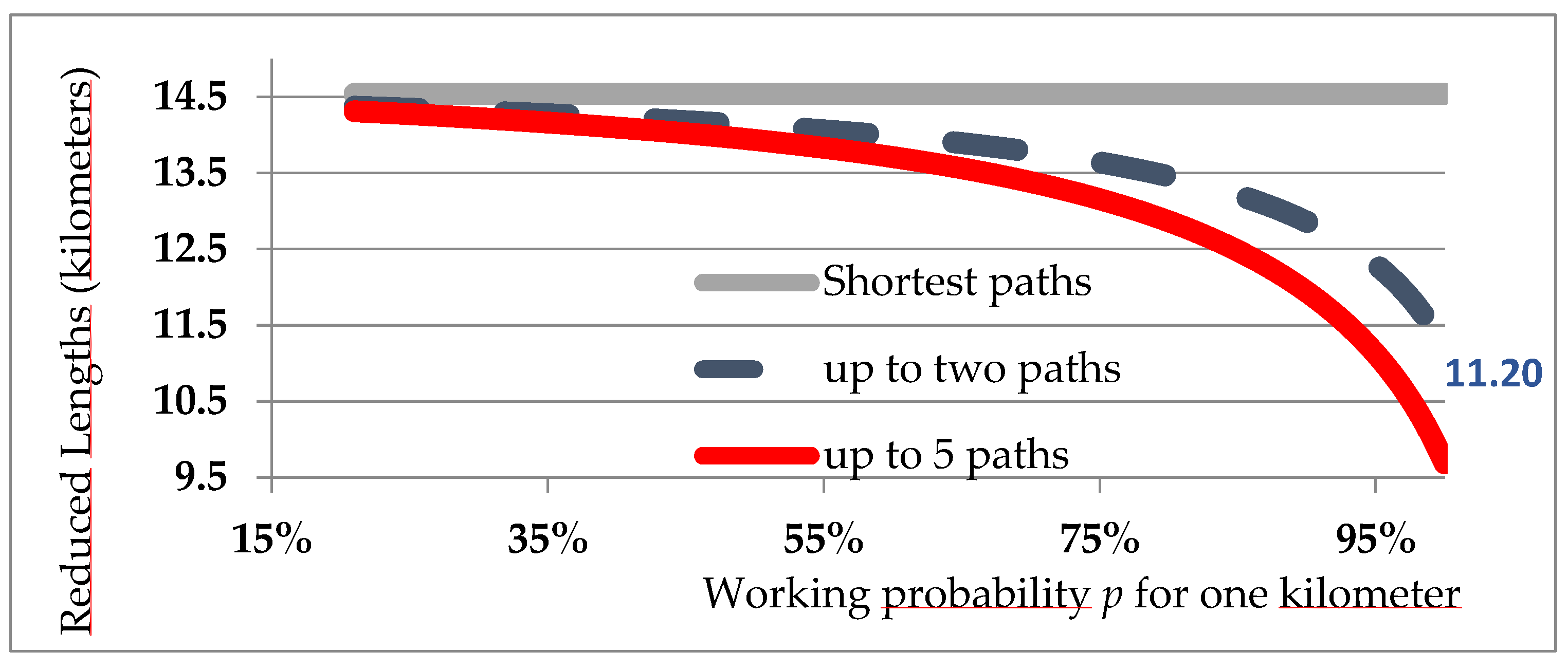
Figure 1.
Average of “OD lengths” on the Rennes bus network according to the operating probability.
The arithmetic average of the shortest paths lengths ( =14.5 kilometers) is displayed by the green horizontal straight line. , the average of the “lengths” of the OD pairs, is displayed by the blue dashed curve (up to two paths) or the red curve (up to five paths). In the case “up to two paths, when p ten. ds to 1, ) tends to 11.2 kilometers which is the average lengths of overlaps - note that for ODs connected by a single path, the entire length of the path is counted as overlap.
When p tends to zero, tends to (no reduction).
Remark.
It’s also interesting to analyze reliability at the level of an individual node (or set of nodes).For a given node, let us define “node reliability” as the average (either geometric or arithmetic) of the R(ω) for all ODs whose origin or destination is that node. Equations (5) and (15) generalize easily to the node level.
5.3. Interpretation of the Increase in Reliability due to Alternative Paths
For a single OD ω, the contribution of the alternative paths is equivalent to an increase of the operating probability p up to a greater probability p’ –or equivalently to a reduction of the failure rate-Log(p) to –Log(p’). The equivalent operating probability p’ with which the reliability of the only shortest path φ1 would become R(ω) is such (after rewriting of Equation (2)) that:
For the whole set of connected ODs, in line with Equation (5), the value p’ which convenes is such that:
N(φ1)= Log’(R(ω))/Log(p’)
5.4. Equations on Unreliability
In this subsection, unreliability, i.e., the quantity “1-reliability”, is decomposed into a product of factors, each of which is related to the unreliability of a path. This decomposition shows the impact of any path.
The event “path j is off” corresponds to the set . An OD is disconnected when the 1st, 2nd, ... kth paths are simultaneously off; this corresponds to the set . The probability of this set is referred as “unreliability”, denoted V(ω), and is equal to 1-R(ω).
Using the chain rule of probability that combines conditional probabilities [38], the unreliability of OD is factored as:
The jth factor of the product, , is equal to =V(φj (ω)) only when the path φj(ω) is disjoint from all previous paths, since in this case the condition” the previous paths do not operate”, is independent of whether φj (ω) operates or not. Otherwise, . The full demonstration is not given here. Intuitively, the condition means that, whatever z (1≤z≤j-1), path z doesn’t operate; now, the more overlaps there are between paths z and j, the more likely it is that the element of z that doesn’t operate belongs to path j, so there is an increase in the probability that path j doesn’t operate.
Let us write this jth factor as:
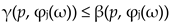
β(p,φj(ω)) is equal to 1 when path φj(ω) is disjoint from all previous paths (independence), less than 1 otherwise. - Recall that )
In order to compare the contribution φj(ω) with that of φ1(ω) let us write:
The denominator of the equation of γ is related to (instead of for β). As the most reliable (thus the least vulnerable) path has been put first, thus:
As the conditional probability is itself a probability distribution, the complement (with respect to value 1) of this jth factor is . This last term corresponds to the increase in reliability for ω when moving from j-1 to j paths - it combines terms already calculated when applying the inclusion/exclusion principle (Equation (13))
Let us note α(p, (ω)) the following ratio:
We can also write:
In information theory, the logarithm in basis 2 of α(p, φ j(ω)) is known as the “pointwise mutual information” between the events: and Sj [39].
Let α(p, φ 1(ω))= β(p, φ 1(ω))= γ(p, φ 1(ω))=1 (whatever p is). The new factorization of V(ω) is:
α(p, φ j(ω)), β(p, φ j(ω)) and γ(p, φ j(ω)) are called “independence coefficient”, “independence degree” and “equivalent degree”.
The inequality β(p,φ j(ω))≤ α(p,φ j(ω)) is obtained by studying Equation (26); β is an increasing function of α.
When path φj is disjoint from the previous paths; the event Sj is independent of then, the condition “|Sj” of Equation (25) has no impact on proba , then α(p, φ j(ω))=1.
Otherwise, the path φj(ω) has a common part with a previous path. α(p, φ j(ω)) and β(p, φ j(ω)) are smaller than 1; we demonstrated in the case j=2, (but the demonstration is not included here), that they decrease when the overlap between φ j and the previous path increases. When path φ j includes a previous path φ j’, φ j does not contribute to unreliability (nore reliability); indeed, in this case thus then:
implying that the jth factor of Equation (19) or Equation (26) equals 1; then α(p, φ j(ω)) = β(p, φj(ω))=0.
In the case j=2 we demonstrated (the demonstration is not included here), that, when p increases from 0 to 1, α and β decrease, from 1 to the proportion, in path φ1, of the number of elements which do not belong to path φ2.
By applying the logarithm function to both members of Equation (26), and replacing 1-R(φ1(ω)) by V(φ 1(ω)) and 1-R(φ j(ω)) by V(φ j(ω)), it comes:
The numbering of the paths 2…k has an impact on the factorization in Equations (24) and (25) and thus on the coefficients α, β, γ, which are therefore not unique; however, when the purpose is to evaluate the gain due an additional path, this new path is in all cases the last one, so the coefficients α, β, γ, for this last path are not disputable. Fortunately, the sum (from 1 to k) of the equivalence degrees γ does not depend on the numbering of paths 2...k: indeed, according to Equation (27), this sum is the ratio Log(V(ω))/Log(V(φ1(ω))). This sum is necessarily less than (or equal to) k. It is as if there were, for ω, only Ʃj=1..k γ(p, φ j(ω)) paths independent and equivalent to φ1.
The geometric mean of the unreliability is obtained by multiplying the products of factors of Equation (26) whatever ω (ω between 1 and NCOD), then taking the NCOD root; its logarithm is obtained by the following equation:
The average (over connected ODs) of the sums (from 1 to k) of the equivalence degrees is the average of the ratios Log(V(ω))/Log(V(φ1(ω))); This average, always between 1 and k, characterizes the impact of alternative paths: it is close to 1 when there are few alternative paths, or when these paths largely overlap, or are much longer than the shortest path.
When the traffic demand per OD is known, unreliability is calculated per user; Equation (28) gives the arithmetic mean of the logarithms of unreliability per user, provided that the coefficient 1/NCOD is replaced by the proportion of the OD demand ω.
6. Results: Application on a City in Brittany
Greater Rennes area in Brittany, France includes 43 communes, served by 148 bus lines; there are 707 bus stops, 680 of which were taken into account here; each bus stop is considered here as as both an origin and a destination, giving 680*679 ODs; the network is represented here.
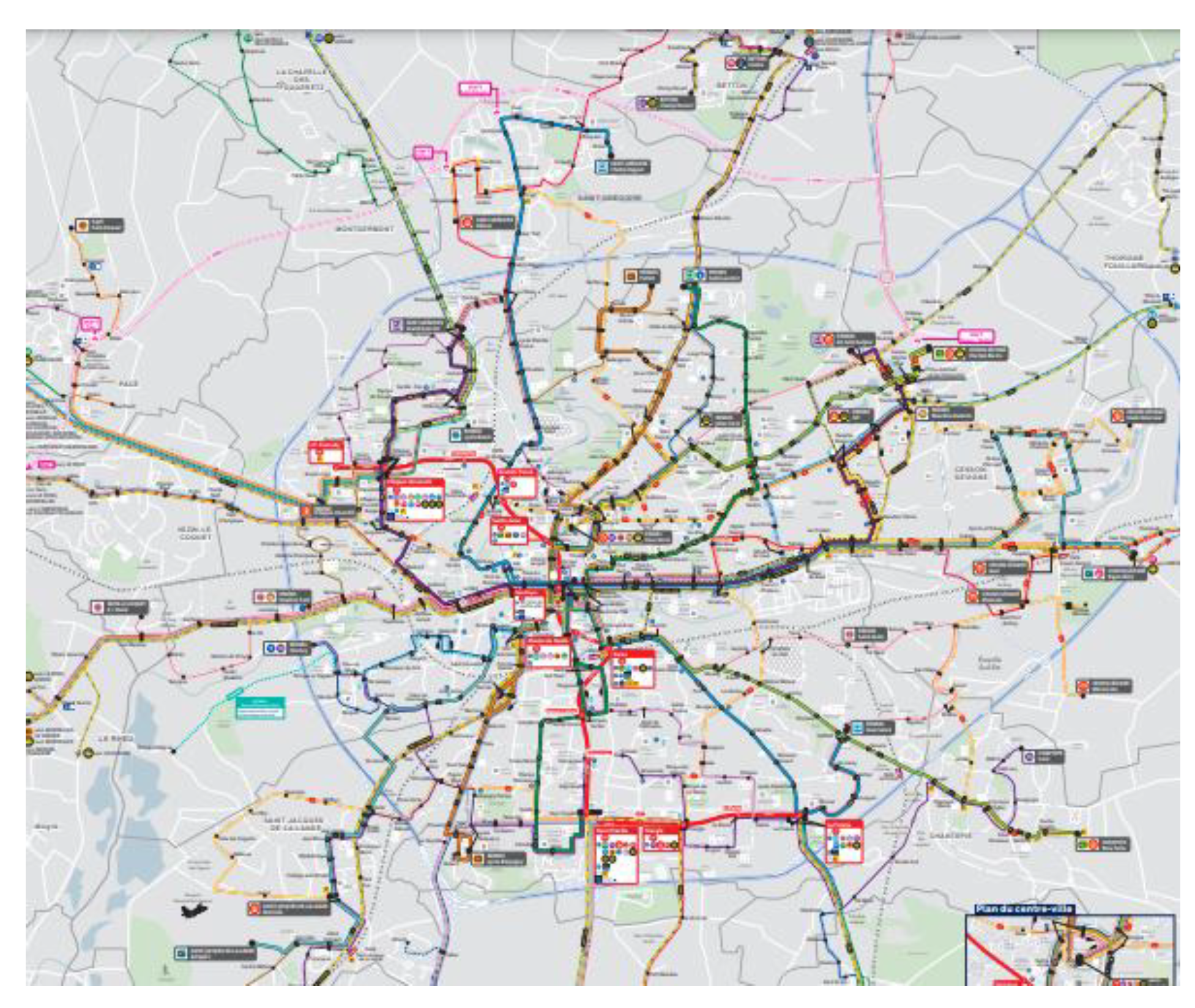
Figure 2.
Map of the Greater Rennes area bus network (extracted from https://www.star.fr).
Figure 2.
Map of the Greater Rennes area bus network (extracted from https://www.star.fr).
The algorithm searched for a maximum of k=5 paths per OD; The criterion to be minimized was the number of connections between buses; the maximum waiting time allowed was one hour; for a user departure time of 8:00, 90.6% of ODs were connected. This might seem low, but it is not unusual for some nodes not to be connected at certain times of the day. An average of 2.48 paths were found per connected OD - here, paths that are identical in space, simply shifted in time, have been eliminated (see Appendix A).
6.1. Reliability due to the Shortest Path and to Alternative Paths for Four Indicators
When several paths connect the same OD, the path placed first (the shortest) depends on the indicator: for the link, bus, length or standard indicators, it is respectively the path with the fewest links, buses taken in succession, the shortest path in length (which is also the least sinuous).
plength was arbitrarily set to 96%, which corresponds to a failure rate λ per kilometer equal to 0.383 (i.e., Log(0.96)= -0.383=- λ ).With the length reliability indicator, the arithmetic mean of the reliability of the shortest paths was 0.581; to facilitate comparisons between indicators (see Appendix B, Equation (29)), Plink , Pbus and Pstandard were chosen to obtain the same average reliability; this occurred for Plink=97.1% , Pbus =83.1% and Pstandard =70.8%. This does not imply that, after inclusion of alternative paths, average reliabilities remain equal, because the gain in reliability due to alternative paths depends on the indicator chosen.

Table 1.
Reliability and Standard Indicators for four indicators (shortest paths and all paths) (no initial/final walks).
Table 1.
Reliability and Standard Indicators for four indicators (shortest paths and all paths) (no initial/final walks).
| Link plink=97.1% |
Bus pbus=80.3% |
Length plength=96% | Standard pstandard=70.8% |
|
| 0.581 | 0.581 | 0.581 | 0.581 | |
| Rarithmetic | 0.680 | 0.673 | 0.674 | 0.680 |
| (*) | 19.40 | 2.53 | 14.54 | 1.65 |
| Average of Average (**) | 23.24 | 2.95 | 15.55 (kms) | 1.71 |
| (***) | 14.09 | 1.89 | 10.91 | 1.22 |
| β | 1.532 | 1.432 | 1.466 | 1.467 |
| γ | 1. 423 | 1.367 | 1.424 | 1.417 |
(*) average, over all connected ODs, of the numbers of elements of the shortest paths, (**) average, over all connected ODs, of the average numbers of path elements per OD, (***) average, over all connected ODs, of the “OD numbers of elements.”.
The average length of the shortest paths is 14.54 kilometers; the average sinuosity for the less sinuous (shortest) paths per OD is 1.65 (see heading “ ” above).
The average, over all connected ODs, of the average numbers of path elements for the OD, is higher than the average on the shortest paths alone (heading ) - alternative paths having a higher number of elements than the shortest paths.
The improvement provided by the alternative paths is equivalent to a reduction in length from =14.54 kilometers (average length of the shortest paths) to 10.91 kilometers ( the average of “OD length”) and a reduction in sinuosity from =1.65 (shortest paths) to =1.22.
The overlaps between the 2.48 paths per connected OD, lead to an average sum of independence degrees between 1.43 and 1.53 (according to the indicator), as if there were, between 1.43 and 1.53 independent (i.e., disjoint) paths per connected OD. The average sum of equivalence degrees is between 1.37 and 1.42, as if there were, on average per OD, between 1.37 and 1.42 paths independent and equivalent to the first (shortest) one.
6.2. Gain When Initial and/or Final Walks Are Allowed
Allowing initial or final walks (here up to 400 meters), increases the percentage of connected ODs (from 90.6% to 90.6% to 96.9%)%; and increases the number of paths per connected OD (from 2.48 to 3.92).
The average, over all connected ODs, of the average numbers of path elements per OD is necessarily higher than the average of the “OD numbers of elements” -see Table 2.
6.3. Reliability Along Bus Line #9
The network is structured around nodes where many bus lines connect. Users entering the network at these nodes are favoured in terms of the bus reliability indicator. Conversely, the closure of such a node has a major negative impact on both the number of connected ODSs and the reliability of those still connected (this point is developed in Appendix C). A study of the evolution of reliability along a bus line (the 8.3 kilometer- long line # 9), shows how to understand and use the various indicators.
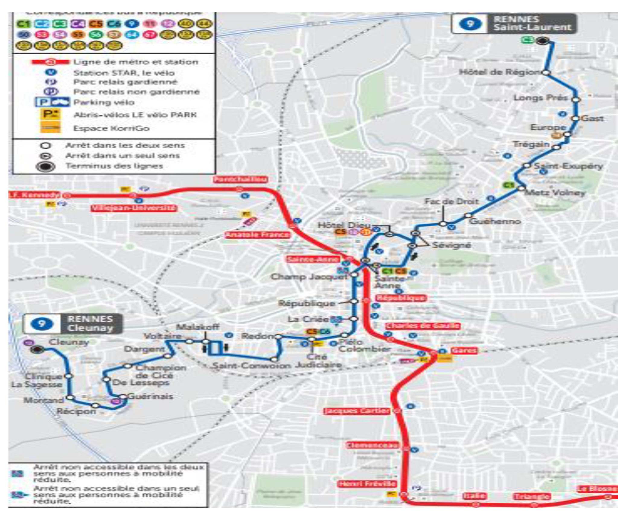
Figure 3.
Line #9 (in blue) in Rennes, from Cleunay to Saint-Laurent (extracted from https://www.star.fr).
Figure 3.
Line #9 (in blue) in Rennes, from Cleunay to Saint-Laurent (extracted from https://www.star.fr).
The node reliability is the arithmetic average of the reliability of ODs that have this node as origin or destination. The reliability of successive bus stops along bus line # 9 is shown in Figure 4 for four reliability indicators.
When a node (a bus stop) is served by very many lines, the shortest paths from this node to very many destinations consist in a single bus. These shortest paths have a single element for bus reliability, resulting in a high bus reliability indicator (shortest paths only). This is particularly the case at “République”, with 19 bus lines. The other bus stops on line #9 generally have a bus reliability (shortest paths only) of just over 0.6, (at pbus =80%), slightly higher than the average bus reliability (shortest paths only) for the whole network (0.581); this is due to the fact that the density of bus lines is higher in the city (where line #9 is located) than in the rest of Greater Rennes.
The increase in bus reliability between the curves (Bus 80% shortest path) and (Bus 80% all paths) is due to alternative paths. The existence of alternative paths is favored when several lines serve a bus stop, implying several ways to reach it. For such nodes, the bus reliability indicator (all paths) is high. This is the case at “Cité Judiciaire” and “Hôtel Dieu”, served by 5 lines as shown in Figure 3.
The standard indicator is close to the bus reliability indicator, firstly because it has been calibrated to be equal to it, on average over the network, and secondly because, for an OD, a good (respectively bad) offer generally allows more direct (respectively less direct) paths, which results in a high (respectively low) standard indicator, as it is the case for the bus reliability indicator. We note that, at République, the standard indicator is not as high as bus reliability, perhaps because the paths are not as direct, due to the presence of the river “La Vilaine” which imposes topological constraints on the road network
Length reliability is greater than 0.736, higher than that of the Rennes network (0.674). Indeed, as line#9 is more central than average, the paths to or from a node on this line are shorter than average. This is particularly true for nodes that are central to line#9.
7. Limitations and Future Work
This work has a number of limitations, which can be overcome in future research.
- Regarding the shortest path algorithm. The introduction of a stochastic term in the travel time would make the connections between buses more realistic. On the other hand, certain paths should be eliminated when they include irrelevant detours, whose sole purpose is to circumvent the maximum waiting time constraint, by replacing part of the waiting time with unnecessary travel time on these detours. This could be avoided by calculating the shortest paths in space (without time constraints) - these paths have no detours - and then proposing the elimination of paths in space-time that are much longer than the shortest paths
- Regarding the network reliability. The geometric average of ODs reliability over-weights ODs with very low reliability; conversely, the geometric average of ODs unreliability over-weights ODs with very high reliability. this argues in favour of replacing geometric averages with arithmetic averages.
- Regarding the ODs with the poorest service. Our approach doesn’t tell us why certain ODs aren’t connected at a given time. An additional tool is needed to propose either an increase in frequencies, the creation of a new line or the extension of an existing line.
8. Conclusions
In this paper, we investigated the connectivity reliability in a public transportation network, by examining, on the basis of real lines and schedules, the {space-time} paths that connect origins and destinations. A shortest path algorithm provides, for each Origin-Destination pair, up to ‘k’ paths in the space-time domain. The reliability of a path is a power function of the reliability of its elements. The length of a path appears equal to the opposite of the logarithm of the path reliability, divided by the failure rate (which is the opposite of the logarithm of the reliability of a path element). The “OD number of elements” or the “OD length”, a new concept, is defined as the opposite of the OD reliability logarithm, divided by the failure rate. When several paths connect an OD, the OD length is less than the length of the shortest path –the reduction in length characterizing the contribution of alternative paths. This extends to the average length over all connected ODs, provided the geometric average is taken into account.
The “standard indicator” is based on the ratio {actual number of kilometers/Euclidean distance} of a path, i.e., its sinuosity. For an OD, the more alternative paths there are in time or space, the higher the standard indicator, the less “OD sinuosity”- This new concept makes it possible to compare the equity of transport supply on different ODs, whatever their Euclidean length, or even to compare different networks. Service improvement projects can be compared on the basis of their performance against this indicator. Fleet managers could define an expected quality of service per OD by a threshold on “OD sinuosity”, and select the project that leads to the largest number of ODs below this threshold (or to the largest number of users concerned, when the demand per OD is known).
Depending on the type of failure, reliability depends on the availability of links, buses, bus stops, or of the successive kilometers of the path. Then, the shortest path is either the shortest path in terms of number of links, buses, stops or length.
In Greater Rennes area (Brittany) the shortest paths connecting the ODs have an average length of 14.54 kilometers. The increased reliability obtained with the alternative paths is that which would have been obtained with a single path reduced in average, to a length of 10.91 kilometers (calculated with a reliability probability of 0.96 per kilometer). While the actual average sinuosity of the shortest paths is equal to 1.65, it is reduced to 1.22 with the alternative paths.
Unreliability is defined here as one minus reliability. The geometric mean of OD unreliability is decomposed into a product of factors, each factor being the unreliability contributed by a path in an OD. This is valid even when paths overlap, thanks to a new concept, the “degree of independence” (between 0 and 1 for each path), which measures the overlap between paths. The more overlaps there are, the lower the degree of independence. The “degree of equivalence”, combines the degree of independence with the possibly lower reliability of the alternative path (compared with the shortest path). In the application, there were, in average, 2.48 paths (including overlaps) per connected OD, but the sums of the degrees of equivalence, was only, in average 1.42.
Author Contributions
Conceptualization and methodology (N.B), reliability indicators (N.B.; T.C. and S.M.H.M-M and MA); software (N.B. and M.A.) ; link with probability and information theory S.M.H M-M; writing, N.B. ; data collection, N.B. ; data processing , M.A.; supervision, T.C.. All authors have read and agreed to the published version of the manuscript:
Acknowledgments
Authors thank KEOLIS-Rennes for the data of the STAR network
Conflicts of Interest
The authors declare no conflicts of unterest.
Nomenclature
| α(p, φj(ω)): | Independence coefficient of the jth path φj of the OD ω at probability p. |
| β(p, φ j(ω)) : | Independence degree of the jth path φj of the OD pair ω at probability p. |
| γ(p, φ j(ω)) : | Equivalence degree of path φj relative to the shortest path φ1(ω). |
| λ: | Failure rate per unit length, (=-logarithm of the operating probability). |
| λi: | Failure rate per unit length for link ai. |
| φ j(ω) : | jth path connecting the Origin-Destination (OD) pair ω. |
| ω: | An Origin-Destination pair. |
| : | Average number of links (over all ODs) of the shortest paths. |
| ai: | One element of path φ. |
| : | Average number of successive buses (over all ODs) of the shortest paths. |
| Dmin(ω) : | Euclidean distance between the origin and destination of ω. |
| L(ai), L(φ) : | Lengths of element ai, length of path φ. |
| Lstandard(ai, ω): | Length of element ai divided by the Euclidean distance Dmin(ω). |
| Lstandard (φ(ω)) : | Length of path φ(ω), divided by the Euclidean distance Dmin(ω). |
| L’(ω, φ): | “Length” of OD pair ω, at probability level p. |
| : | Average number of kilometers (over all ODs) of the shortest paths. |
| M: | Number of elements of the network. |
| N(φ) : | Number of elements of path φ. |
| N’(ω,p): | “OD number” of elements for OD ω. |
| : | Average number of elements (over all ODs) of the shortest paths. |
| : | Average of “OD numbers” of elements (over all ODs), at probability p. |
| NCOD: | Number of connected Origin-Destination pairs. |
| : | Average number of bus stops (over all ODs) of the shortest paths. |
| p, p (ai) : | Operating probability; operating probability for element ai. |
| pbus,pstop, plink: | Operating probability for a bus, a bus stop, a link. |
| plength : | Operating probability per unit of length. |
| pstandard: | Chosen parameter for the standard indicator. |
| ri: | Count for element ai, when its operating probability differs from p. |
| R(φ), R(ω): | Reliability for path φ, for an Origin-Destination pair ω. |
| Rarithmetic (p): | Arithmetic mean of OD reliability (over connected ODs) at probability p. |
| Rgeometric (p): | Geometric mean of OD reliability (over connected ODs) at probability p. |
| : | Geometric mean (over all connected ODs) of the shortest path reliability. |
| : | Arithmetic mean (over connected ODs) of the shortest path reliability. |
| Rbus, Rlink Rstop: | Reliability indicators based on buses, links or stops availability per path. |
| Rlength: | Reliability indicator based on the length of a link. |
| Rstandard: | Approachability indicator based on the path sinuosity. |
| Sj , : | Sets of network states such that path φj is operating (resp. not). |
| : | Average sinuosity (over all ODs) of the shortest paths. |
| V(φ), V(ω) : | Unreliability (i.e., One minus Reliability) of path φ or of the OD pair ω. |
| Vgeometric(p) : | Geometric mean of unreliability (over connected ODs) at probability p. |
Appendix A : k Shortest Paths Algorithm in a Public Transportation NetworkA
The algorithm is based on the Dijkstra algorithm [40], and provides the shortest paths from an origin to all destinations for a given departure time. To take account bus schedules, the network is modeled in space-time by nodes and links, each node or link being time-stamped and having topological coordinates. Origins and destinations are nodes in space; the departure time is assigned to origins. Each time, throughout the day, that a bus arrives at (or departs from) a stop, a node is created in space-time; Links between these nodes model the bus moving. Other links, modeling waiting time, connect the various nodes in {space x time corresponding to a bus stop. Initial walk links are optionally created between the origin and each nearby bus stop (whose Euclidean distance is less than a certain threshold); final walk links are also optionally created between each bus stop and nearby destinations.
To obtain the k shortest paths, we created k occurrences (i.e., duplicate k times) of most of nodes and links. The label-setting used in the Dijsktra algorithm is modified accordingly, and a loop prevention module is added.
During the step-by-step creation, by the algorithm, of a path from the origin to a destination, at a certain time, the possibility of continuing the path by connecting to another bus line is subject to the following conditions:
- Waiting time must be positive, and below a predefined threshold. This threshold applies either to the total waiting time since the origin of the path, or to the local waiting time, at every bus stop - this second option was taken here in the numerical application.
- Only the first available bus on each line is considered- There is no point in waiting for taking the second bus,
- When two bus lines share a common trunk, a user doesn’t alternate between the two lines. Alternation is avoided by rejecting the further creation of a path that is spatially identical to a previously found path. Note that this rejection implies rejecting paths that are identical in space but offset in time- these rejected paths can be easily reintroduced afterwards.
However, a user usually waits for taking the second available bus if the line of the second bus is more direct to the final destination. This path, which begins identically to the path taking the first bus, is unduly rejected by the previous rule. Instead of this rule, another rule to avoid alternation consists in rejecting the further creation of a path when it would imply that, in the path, the same bus line is taken twice (or, on option, three times); the paths rejected by the first rule are no more rejected; however this second rule may unduly eliminate certain paths in certain, admittedly rare, cases,: let’s consider a network made up of a North- South radial bus line, crossing a circular bus line. Let’s consider an OD whose origin is located on the circular bus line, at a stop closed to the first stop where the two lines connect; and whose destination is also located on the circular bus line, at a stop closed to the second stop where the two lines connect. The user may start his path on the circular line, abandon it to take the radial line, then take the circular line a second time to reach his destination. Such a path is unfortunately eliminated by the second rule. So we need to run the algorithm twice, once with the first rule, once with the second rule, and then combine the best results from the two runs.
Appendix B . Adjustments of pstandard
B1.Adjustment of Pstandard for easier Comparison Between the Standard Indicator and the Bus Reliability Indicator
pstandard is adjusted so as to equalize the geometric means (over all connected ODs, considering only one path, the most reliable per OD) of the two indicators. Applying Equation (1) to both indicators, it comes that pstandard must be the solution of:
Where and are the arithmetic means (calculated by considering only the shortest paths) of the number of buses to be taken per path, and the sinuosity of the paths.
B2. Adjustment of pstandard According to the Payoff Between Sinuosity and Number of Independent Paths
Improving the service to an OD pair ω can be done by creating a new route, less sinuous, by increasing the frequency or the number of paths connecting ω. The first decision reduces users’ travel time; the last two reduce their waiting time. Equaling the impacts of these decisions on the standard indicator makes it possible to determine which increase in frequency or on the number of alternative paths is equivalent to reducing sinuosity.
The bus fleet manager might select pstandard such that the standard indicator of an OD-pair ω (connected by k independent paths, each of sinuosity s) is equivalent to the one of OD-pair ω’, (connected by a single path of sinuosity 1). Since independence allows the use of a multiplicative scheme on unreliability, pstandard must be such that:
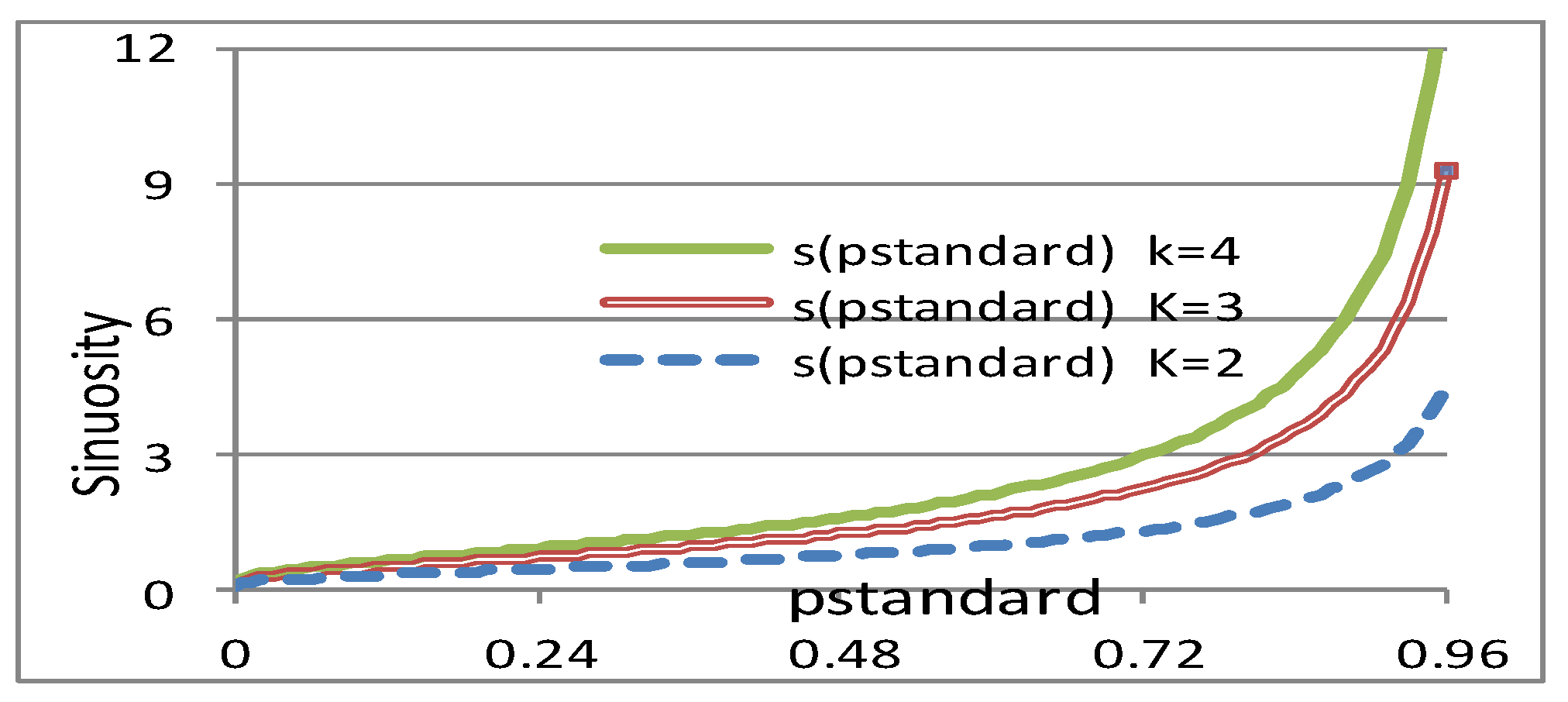
This equation is derived from Equations (1) and (12). For a given s>0 and k>1, Equation (30) has a unique solution 0<pstandard <1 (discarding the trivial but irrelevant solutions pstandard =0 or pstandard = 1).
For a given number of (independent) paths k, the function s(pstandard |k), which gives s with respect to pstandard, is obtained from Equation (30) as:
Figure 5 gives pstandard (on the X-axis) according to the sinuosity (on the Y-axis) for different values of k. The higher the sinuosity, the higher pstandard should be taken.
Figure 5.
Sinuosity according to the value of pstandard and of the number of independent paths.
Appendix C. Impact of Closing One Bus Stop on Network Reliability
“Closing” means here that each bus line passing by the closed bus stop is divided in two: one ending at the stop just before the closed bus stop; the second beginning at the first bus stop after the closed bus stop. Necessarily, some OD pairs are subtracted (those whose origin or destination is the closed bus stop). When there are C bus stops (thus C origins and C destinations) in the network, the number of OD pairs is C*(C-1); when closing a bus stop, it decreases to (C-1)*(C-2) - the decrease is equal to 2*(C-1), relative decrease is 2/C. - the factor 2 is because the closed bus stop is both the origin and the destination of (C-1) OD pairs. The relative decrease is higher than 2/C when possibilities of transfer decrease: for instance let us consider the closing of the 3rd bus stop of the line with no possibility of transfer at the two first bus stops, these two first bus stops would be heavily impacted by the closing of the third. In addition, other OD pairs are disconnected when the waiting time to use a complicated path that get around the closed stop, exceeds the maximum allowed. Let us define the “normalized” decrease as the relative decrease of the number of connected ODs, divided 2/C; this normalized decrease no longer depends on network size; its absolute value and is greater than 1.
We calculated the network reliability and the normalized decrease in connected ODs in eleven cases (each time closing a node on line #9) and plotted both curves on Figure 6: The decreases in reliability and in normalized number of connected OD seem to be roughly proportional - sometimes drastically so when a very important node is closed.
Figure 6.
Network reliability (length indicator, at p=96%) and normalized decrease of connected ODs, for eleven closing of a bus stop of Line #9.
Figure 6.
Network reliability (length indicator, at p=96%) and normalized decrease of connected ODs, for eleven closing of a bus stop of Line #9.
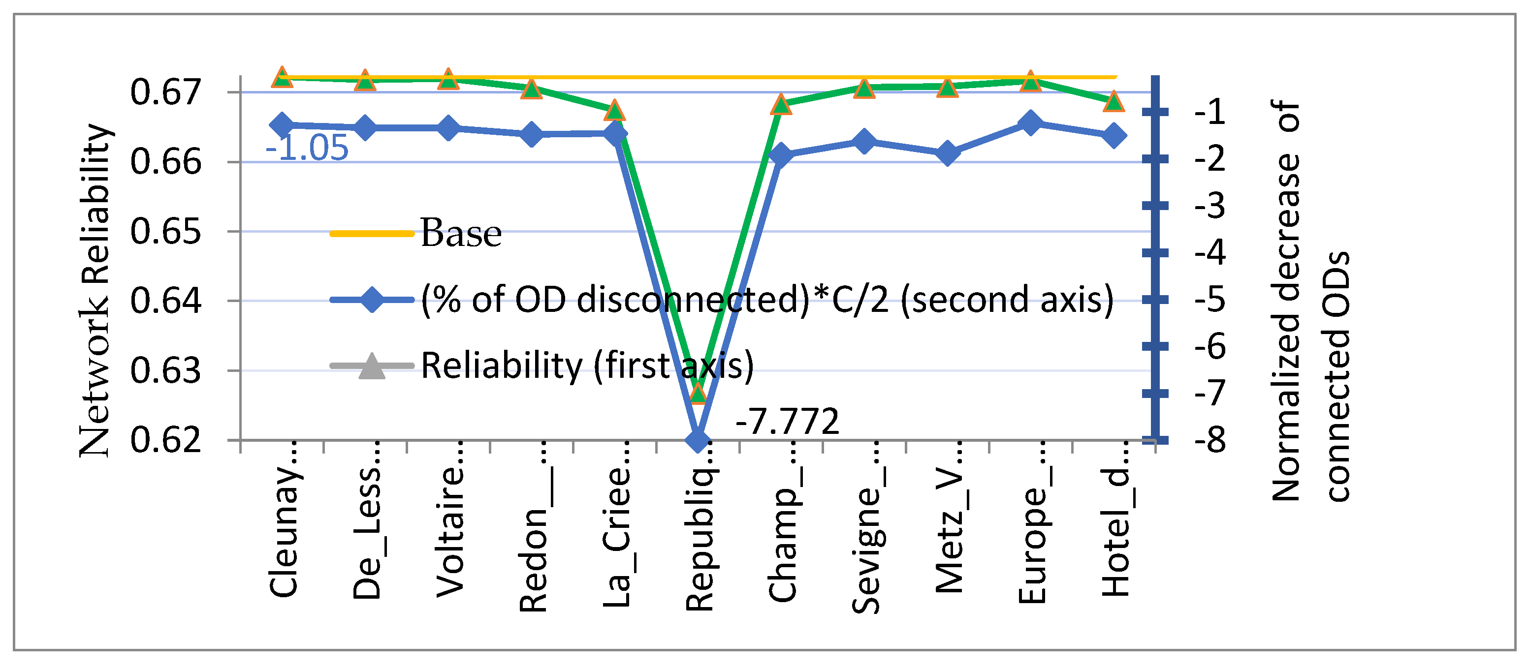
Here no initial / final walk was considered. The normalized decrease varies (in absolute value) between 1.05 (when the terminus “Cleunay”, or many other stops, are closed) and 7.77 (when République is closed); this normalized decrease corresponds to a decrease of the percentage of connected ODs from 90.6% (République open) to 88.5% (République closed).
The network reliability is here the arithmetic average of length reliability for still connected ODs ; with this calculation method, the closure of a secondary stop has practically no impact on the average reliability of the network. When République is closed, it decreases from 0.674 to 0.628 –in addition the average number of buses taken increases from 2.95 to 3.98.
Allowing initial or final walks (up to 400 meters) makes it possible to bypass the closure of “République”– then, the percentage of connected ODs increases up to 96%.
References
- Sakarovitch, M. The k shortest chains in a graph. Transportation Research 1968, 2, 1–11. [Google Scholar] [CrossRef]
- Wakabayashi, H.; Iida, Y. Upper and lower bounds of terminal reliability of road networks: an efficient method with Boolean algebra. Journal of natural disaster science 1992, 14. [Google Scholar]
- Nicholson, A. Assessing Transport Reliability: Malevolence and User Knowledge. Proceedings of the 1st International Symposium on Transportation Network Reliability (INSTR) 2003. [Google Scholar] [CrossRef]
- Mattsson, L.-G.; Jenelius, E. Vulnerability and resilience of transport systems: A discussion of recent research. Transportation Research Part A: Policy and Practice 2015, 81, 16–34. [Google Scholar] [CrossRef]
- Mahdavi-Moghaddam, H.S.M.; Bhouri, N.; Scemama, G. Dynamic Resilience of Public Transport Network: A Case Study for Fleet-Failure in Bus Transport Operation of New Delhi. Transportation Research Procedia 2020, 47, 672–679. [Google Scholar] [CrossRef]
- Bell, M G.H.; Iida.Y. Transportation Network Analysis. Ed. John Wiley & Sons, Ltd. USA. 1997. [CrossRef]
- Liu, J.; Peng, Q.; Chen, J.; Yin, Y. Connectivity reliability on an urban rail transit network from the perspective of passenger travel. Urban Rail Transit 2020, 6, 1–14. [Google Scholar] [CrossRef]
- Soltani-Sobh, A.; Heaslip, K.; Stevanovi, A.; Khoury, J.E.; Song, Z. Evaluation of transportation network reliability during unexpected events with multiple uncertainties. International Journal of Disaster Risk Reduction 2016, 17, 128–136. [Google Scholar] [CrossRef]
- Oliveira, E. L,; Portugal, L-D-S; Porto Junior, W. Indicators of reliability and vulnerability: Similarities and differences in ranking links of a complex road system. Transportation Research Part A: Policy and Practice 2016, 88, 195–208. [Google Scholar]
- Kim, H.; Kim, C.; Chun, Y. Network Reliability and Resilience of Rapid Transit Systems. The Professional Geographer 2016, 68, 53–65. [Google Scholar] [CrossRef]
- D’Este, G.M.; Taylor, M.A.P. Network vulnerability: an approach to reliability analysis at the level of national strategic transport networks. In: The Network Reliability of Transport, Bell, M.G.H., Iida, Y. (Eds.), Proceedings of the 1st International Symposium on Transportation Network Reliability (INSTR), Emerald, Bingley, U.K., 2003 pp. 23–44.
- Jenelius, E.; Petersen, T.; Mattsson, L.-G. Importance and exposure in road network vulnerability analysis. Transportation Research Part A 2006, 40, 537–560. [Google Scholar] [CrossRef]
- Connors, R., D.; Watling, D.P. Assessing the demand vulnerability of equilibrium traffic networks via network aggregation. Networks and Spatial Economics 2014, 15, 365–395. [Google Scholar] [CrossRef]
- Rodriguez-Nunez, E.; Garcia-Palomares, J. C. Measuring the vulnerability of public transport networks. Journal of Transport Geography 2014, 35, 50–63. [Google Scholar] [CrossRef]
- Yap, MD.; van Oort, N.; van Nes, R.; van Arem, B. Identification and quantification of link vulnerability in multi-level public transport networks: a passenger perspective. Transportation 2018, 45, 1161–1180. [Google Scholar] [CrossRef]
- Ye, Q.; Kim, H. Assessing network vulnerability using shortest path network problems. Journal of Transportation Safety & Security 2019. [Google Scholar] [CrossRef]
- Cats, O.; Erik Jenelius, E. Beyond a complete failure: the impact of partial capacity degradation on public transport network vulnerability. Transportmetrica B: Transport Dynamics 2018, 6, 77–96. [Google Scholar] [CrossRef]
- Liu J, Schonfeld, P.M.; Yin, Y.; Peng, Q.; Ranjitkar P. Effects of Link Capacity. Reductions on the Reliability of an Urban Rail Transit Network. J Adv Transport 2020, 1–15. [CrossRef]
- Liu, J.J.; Schonfeld, P.M.; Zhan,S.; Du, B.; He, M.; Wang, K.C.P.; Yin, Y. The Economic Value of Reserve Capacity Considering the Reliability and Robustness of a Rail Transit Network.’Journal of Transportation Engineering, Part A: Systems 2023, 149. [CrossRef]
- Taylor, M.A.P.; D’Este, G.M. Transport network vulnerability: a method for diagnosis of critical locations in transport infrastructure systems. In: Critical Infrastructure. Murray, A.T., Grubesic, T.H. (Eds.), Springer Berlin, Heidelberg, Germany, 2007 pp.9–30.
- Zang,Z.; Xu, X.; Qu, K.; Chen, R.; Chen, A. Travel Time reliability in transportation networks: A review of methodological Developments. Transp. Research part C. Emerging Technologies 2022 143. [CrossRef]
- Taylor, M.A. P. Travel through time: The story of research on travel time reliability. Transportmetrica B 1. 2013, 174–194. [Google Scholar] [CrossRef]
- Benezech, V.; Coulombel, N. The value of service reliability. Transportation Research Part B 2013, 58, 1–15. [Google Scholar] [CrossRef]
- Muñoz, J. C.; Soza-Parra, J.; Raveau, S. A comprehensive perspective of unreliable public transport services costs. Transportmetrica A Transport Science 2020, 16, 734–748. [Google Scholar] [CrossRef]
- Artan, M.S.; Şahin, I. A stochastic model for reliability analysis of periodic train timetables. Transportmetrica B: Transport Dynamics 2023, 11, 572–589. [Google Scholar] [CrossRef]
- Shelat, S.; Cats, O.; van Oort, N.; van Lint, J. W.C. Evaluating the impact of waiting time reliability on route choice using smart card data. Transportmetrica A: Transport Science 2023, 19, 2. [Google Scholar] [CrossRef]
- Khani, A. An onroute shortest path algorithm for reliable routing in schedule-based transit networks considering transfer failure probability. Transportation Research Part B 2019, 126, 549–556. [Google Scholar] [CrossRef]
- Redmond, M.; Campbell, A.M.; Ehmke, J.F. Reliability in public transit networks considering backup itineraries. European Journal of Operational Research, Elsevier, 2022, 300, 852–864. [Google Scholar] [CrossRef]
- Clark, S.; Watling, D. Modelling network reliability under stochastic demand. Transp. Res. Part B 2005, 39, 119–140. [Google Scholar] [CrossRef]
- Chen, A.; Yang, H.; Lo, H.K.; Tang, W.H. Capacity reliability of a road network: an assessment methodology and numerical results. Transp. Res. B 2002, 36, 225–252. [Google Scholar] [CrossRef]
- Yang, H.; Lo, K. K.; Tang, W. H. Travel time versus capacity reliability of a road network. Transportation Research Board 79th Annual Meeting, 2000. [Google Scholar]
- Kim, H.; Song, Y. Examining accessibility and reliability in the evolution of subway systems. J. Public Transp. 2015, 18, 89–106. [Google Scholar] [CrossRef]
- Bimpou,K.; Ferguson, N.S. Dynamic accessibility: Incorporating day-to-day travel time reliability into accessibility measurement. Journal of Transport Geography.
- Kim, H.; Song, Y. An integrated measure of accessibility and reliability of mass transit systems. Transportation 2018, 45, 1075–1100. [Google Scholar] [CrossRef]
- Taylor, M.A.P. Dense network traffic models, travel time reliability and traffic management. Ii: Application to Network reliability. Journal of Advanced Transportation 2010, 33, 235–251. [Google Scholar] [CrossRef]
- Shannon, C.E.; Weaver,W. The mathematical theory of communication, University of Illinois, Urban III, USA, 1949.
- Van Lint, J.H.; Wilson, R.M. A Course in Combinatorics. Cambridge University Press, The U.K., 1992 .
- Feller, W. An Introduction to Probability Theory and Its Applications, volume 1, 3rd ed., New York / London / Sydney: Wiley, USA, 1958 ISBN 978-0-471-25708-0 .
- Fano, R.M. Transmission of Information: A Statistical Theory of Communication. Chapter 2 MIT Press, Cambridge, MA, USA, 1961 .
- Dijkstra, Ed.W. A note on two problems with connection to graphs. Numerische Mathematik 1959, 1, 269–271. [Google Scholar] [CrossRef]
Figure 4.
Bus reliability, length reliability and standard indicator for the nodes of Line #9 (no initial/final walks; probability values p adjusted for comparisons).
Figure 4.
Bus reliability, length reliability and standard indicator for the nodes of Line #9 (no initial/final walks; probability values p adjusted for comparisons).
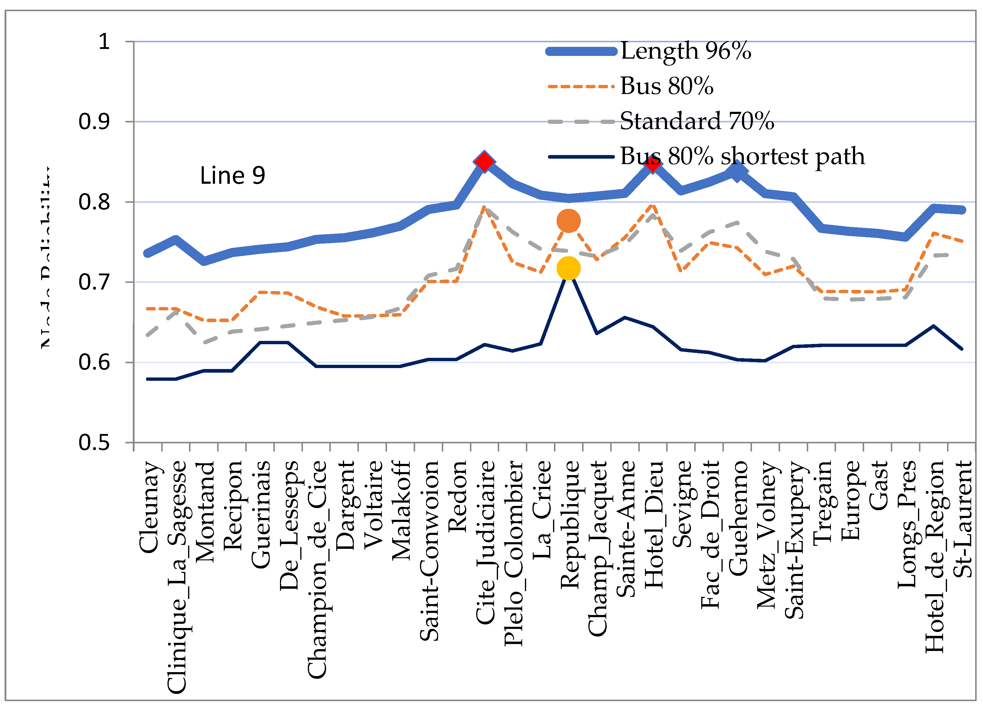
Table 2.
Average of the average numbers of path elements per OD, and average of the “OD numbers of elements”, for 4 indicators (initial/final walks allowed).
Table 2.
Average of the average numbers of path elements per OD, and average of the “OD numbers of elements”, for 4 indicators (initial/final walks allowed).
| Link plink=97.1% | Bus pbus=80.3% |
Length plength=96% | Standard pstandard=70.8% | |
| Average of Average | 22.09 | 2.12 (*) | 14.52 | 1.681 |
| 12.26 | 1.668 | 9.99 | 1.044 |
(*) in average, 0.59 initial or final walks have to be added to the 2.12 buses per path.
Disclaimer/Publisher’s Note: The statements, opinions and data contained in all publications are solely those of the individual author(s) and contributor(s) and not of MDPI and/or the editor(s). MDPI and/or the editor(s) disclaim responsibility for any injury to people or property resulting from any ideas, methods, instructions or products referred to in the content. |
© 2024 by the authors. Licensee MDPI, Basel, Switzerland. This article is an open access article distributed under the terms and conditions of the Creative Commons Attribution (CC BY) license (http://creativecommons.org/licenses/by/4.0/).
Copyright: This open access article is published under a Creative Commons CC BY 4.0 license, which permit the free download, distribution, and reuse, provided that the author and preprint are cited in any reuse.


