
Submitted:
31 October 2024
Posted:
08 November 2024
You are already at the latest version
Abstract
With the rapid development of urbanization, the ecological environment is being destroyed. Taking Barcelona Metropolitan Region as an example, this paper established an ecological environment quality assessment system suitable for different time and region based on remote sensing to evaluate it from 2006 to 2018. And built various OLS models to analyze multiple variables affecting the ecological environment. Finally, the characteristic triangular space structure was used to explain the interaction between the two key variables. The results showed that the ecological quality was unevenly distributed. The largest green space contributed the most ecological benefits, but its area was decreasing and its shape was more fragmented. NDVI was the most significant natural variable related to the distribution of green space. Precipitation was the most closely related climate factor to NDVI. And there was a complex two-way interaction mechanism between the two, and its boundary value was getting higher and higher. In conclusion: The environmental quality of BMR needs to be improved. There is a two-way relationship between the two key factors. The characteristic triangle can successfully explain the interaction mechanism between precipitation and NDVI.
Keywords:
ecological environment quality
; remote sensing
; climate change
; precipitation
; NDVI
; urban expansion
; characteristic triangle
; sustainable development
1. Introduction
In the past few decades, environmental assessment, as an important part of environmental management, has gradually attracted people’s attention [1]. People have realized the impact of human activities on environmental change and recognized the key role of environmental assessment in studying the process of environmental change [2]. In today’s world, with the rapid development of urbanization and social and economic construction, the ecological environment has been severely damaged by human activities, and ecological problems such as soil erosion, land salinization and desertification, and a sharp decline in plant and animal diversity have also increased [3,4]. At the same time, with the deterioration of the ecological environment, natural disasters and extreme climates such as floods, droughts, global warming, and high temperature heat waves have occurred frequently [5,6,7]. A good ecological environment is the basis for sustainable social development and human survival. The deterioration of the ecological environment has seriously affected the development of human society and people’s health. We must pay attention to solving ecological and environmental problems while maintaining urban construction and economic development, as well as the continuous progress of science and technology. Only in this way can we achieve a harmonious coexistence between man and nature, reduce the frequent occurrence of natural disasters and extreme weather, and protect people’s health and the sustainable use of natural resources [8].
The scientific evaluation of the ecological environment and the rational optimization and regulation of its pattern are not only hot issues in the field of climate and environment research, but also urgent needs for ecological economic development and ecological civilization construction [9]. At present, satellite remote sensing earth observation systems have been widely used in the field of ecological environment due to their advantages of macro, rapid and real-time. The use of various remote sensing indicators to monitor and evaluate natural forests, grasslands, urban artificial ground, water bodies, and even ecosystems in the entire region has become an important part of the field of ecological environment protection [10]. With the development of “3S” technology (remote sensing, geographic information system and global positioning system), many scholars have begun to use RS and GIS technology to obtain ground information, combined with mathematical models and statistical analysis methods, from single factors to multiple factors, to conduct comprehensive evaluation of the ecological environment in different regions and scales [11,12]. In 2009, Ivits et al. used SPOT image data and the vegetation index NDVI as an ecological indicator to evaluate the ecological environment of forests and farmland bird habitats in China [13]. Marllu J et al. used a variety of ecological factors such as vegetation sensitivity index and ecological isolation index to construct an evaluation system to evaluate the quality of urban ecological environment [13]. Studies have shown that the ecological quality status obtained by this method has reference significance for relevant decisions on urban land use planning. In 2013, Xu Hanqiu proposed a new remote sensing ecological index (RSEI) based on remote sensing information technology. The index couples four indicator factors: vegetation index, humidity component, surface temperature and soil index, and then uses principal component transformation to integrate more complete information in the region [15]. This study used the RSEI index and China’s traditional EI index to analyze the ecological environment in areas with severe soil erosion in Fujian Province, providing prediction and dynamic change analysis, and making up for the shortcomings of the EI index. In 2021, Wang Zi selected four phases of Landsat series remote sensing images as data sources, added research indicators that meet the characteristics of saline-alkali land in the research object, and comprehensively evaluated the ecological environment quality of the Chahan Nur Basin from 1992 to 2020, and analyzed the driving factors of changes in ecological environment quality [8]. In 2022, Hou Yifeng et al. analyzed the evolution of land cover changes in the Tarim River Basin over the past 30 years and explored the contribution of transformations between different land types to the ecological environment [16].
Normalized Difference Vegetation Index (NDVI) can be used to detect plant biomass, vegetation coverage, growth status, etc. It is the best indicator factor reflecting the vulnerability of regional ecological environment and is also the most widely used index in vegetation remote sensing monitoring research [17,18]. Vegetation occupies a major position in the earth’s terrestrial ecosystem and is an important medium for the material and energy cycle of the earth’s ecosystem [19]. NDVI changes play a guiding role in the study of regional ecological environment evolution [20]. High NDVI values usually indicate high vegetation density and healthy growth, which helps to improve the resilience and biodiversity of the ecosystem [21]. In 2004, Wessels et al. studied the land degradation effects caused by human activities in the former homeland area of northern South Africa and found that NDVI values can indirectly reflect the health of the soil and thus judge the quality of the local ecosystem. There is a positive correlation between them [22]. In addition, NDVI can effectively reflect the seasonal changes and long-term trends of vegetation and is effectively applicable to the monitoring and evaluation of different ecosystems [23]. Goward and Prince studied the relationship between NDVI and vegetation net primary productivity (NPP) and found that NDVI can be used as an alternative indicator of NPP to assess the health of the ecological environment [24]. De Jong et al. studied the impact of grazing on vegetation and erosion in Paraguay and found that NDVI monitoring can effectively evaluate the effect of ecosystem restoration [25]. In 2020, Ren Jie systematically studied the driving factors and influence of the evolution of the surface ecological environment in the western region of the Yili Basin based on NDV and combined with the ILUCC theory, and found that the lower the NDVI, the more sensitive the ecological quality [26]. However, at present, scholars have not yet formed a unified standard for evaluating the quality of the ecological environment. The commonly used land weight index is only a numerical value [8,11,12,13,14,15,16,23,24,25,26], which can only generally describe the ecological status of a region in a certain period, and cannot analyze the spatial changes of the ecological environment in different periods. At the same time, different scholars consider this weight index from different perspectives. Therefore, trying to find a more scientific and reasonable indicator system to evaluate the ecological environment quality of the metropolis, which can be applied to changes in land use types in different periods and regions, is one of the important tasks of this study.
Many of the above studies have shown that NDVI is an extremely important factor that affects and reflects the ecological environment quality of a region. Therefore, it is particularly important to analyze the factors that can have the most direct impact on NDVI and thus indirectly regulate ecological quality. Many studies have shown that temperature, soil properties, topography and human activities are factors that can directly affect NDVI changes [27,28,29,30,31,32], but there is a more intimate and complex relationship between NDVI and precipitation. Generally speaking, sufficient precipitation can promote plant growth, increase biomass and NDVI values. Conversely, drought and insufficient precipitation will reduce NDVI values [21,33]. However, the relationship between precipitation and NDVI still has obvious differences in different regions and times. Mu Shaojie et al. found [34] that there is a significant time lag effect in the response of NDVI to precipitation in grassland areas. Liu et al. studied the vegetation dynamics of the Amazon rainforest and found that even in areas with abundant precipitation, seasonal precipitation changes can still cause significant fluctuations in NDVI [35]. Xu Yue et al. also proposed that the response rate of NDVI to precipitation changes in different seasons is also different [36]. In previous works, the authors also believed that the effect of precipitation on plant cover is a highly complex factor and it is difficult to determine the true relationship between them, but in fact precipitation does provide a great help to the growth of vegetation [27]. From the current research status, the relationship between precipitation and NDVI is still an unresolved topic.
Based on the above, this article will build a more scientific and reasonable evaluation system based on NDVI, which can be applied to dynamic ecological environment quality in different metropolitan areas and periods, and use this system to evaluate the ecological environment quality of Barcelona Metropolitan Region. Secondly, we will comprehensively analyze the various natural and human factors that can affect NDVI. Most importantly, the relationship between precipitation and NDVI must be deeply analyzed. We try to discover some laws and inspirations for this unresolved topic to a certain extent.
2. Materials and Methods
2.1. The Field of Study
The Barcelona Metropolitan Region (BMR, Figure 1) is located in the northeast of the Iberian Peninsula, in the center of the Mediterranean corridor connecting Spain to the rest of continental Europe, and it has a typical Mediterranean climate. It is the largest metropolitan area in Catalonia and serves as its political, economic and cultural core. It covers an area of approximately 3224.7 km2 and contains 164 municipalities. With a population of around 5.4 million inhabitants, the BMR is the most densely populated metropolitan area in the European Union. The Llobregat and Besòs rivers are the two main rivers that flow through the metropolitan region of Barcelona. The coastal and pre-coastal mountain ranges delimit the coastal and pre-coastal depressions where the main population centers are located. It includes the more densely populated Barcelona Metropolitan Area (BMA), about 636km2, covering the city of Barcelona and 35 surrounding towns, with a permanent population of about 4.7 million. The urban core area of Barcelona is about 100 km2, with a population of more than 1.65 million, and a population density of more than 16,500 inhabitants/km2. The Collserola “serralada” (the central part of the coastal mountain range) occupies a central place in the metropolitan area, making it the “green lung” around which the built spaces are located. The Barcelona Metropolitan Territorial Plan (10) pays special attention to the protection of the ecological environment and green spaces of the BMR. The green area of the entire Barcelona Metropolitan Region is about 2514km2, which includes urban parks, suburban parks, forests and protected areas, accounting for about 77.4% of the total area. Based on the above situation, we chose BMR as the study area to evaluate the evolution of its ecological environment quality and analyze the impact of various factors, especially precipitation, on NDVI.
2.2. Methodology
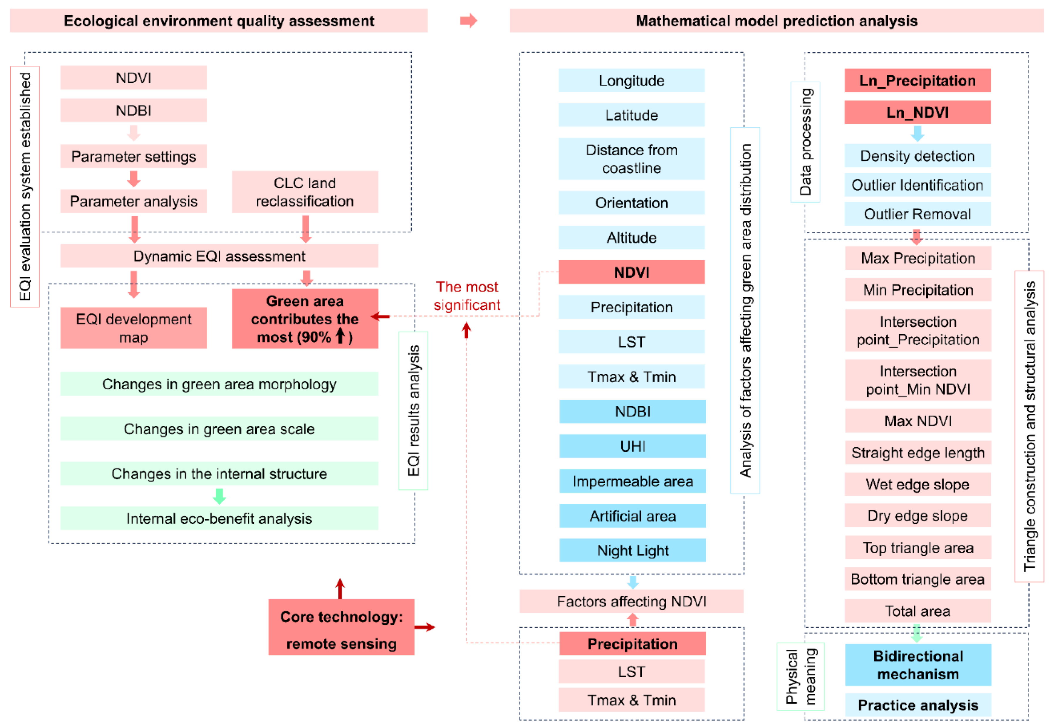
Assessing and analyzing the quality of green ecological environment in metropolitan areas can help protect and restore urban ecosystems, balance species diversity, provide a scientific basis for urban planning, and help formulate reasonable protection and expansion strategies. Studying the changing mechanisms that affect NDVI can enhance the resilience of ecosystems, improve their ability to adapt to extreme climates, and improve the well-being of residents. Corine Land Cover (CLC) provides us with relatively accurate European land cover data with a resolution of 100 meters in 2006, 2012, and 2018 (https://land.copernicus.eu/en/products/corine-land-cover), which records 22 types of green space systems in detail. Based on this dataset, we carried out this study in the following steps.
- First of all, evaluate the Ecological Environment Quality Index (EQI) of BMR. We try to find a more scientific and reasonable indicator system to evaluate the ecological environment quality of metropolises, which can adapt to changes in time and the evaluated regions. To complete this evaluation, we need to achieve the following aspects.
- For the convenience of analysis, we classified the land use coverage of BMR according to the land type classification of CLC.
- Then, we extracted the difference (NDVIaverage-NDBIaverage) of the annual average values of NDVI and NDBI for each type of land in 2006, 2012 and 2018 after reclassification. The MODIS_MOD13Q1 (https://lpdaac.usgs.gov/products/mod13q1v006/) dataset provides relevant remote sensing image data with a resolution of 250 meters.
- Set EQI evaluation parameters. Normalized Difference Vegetation Index (NDVI) is the best indicator of regional ecological environmental vulnerability. In previous studies, the authors believed that the tall tree canopy in summer would make the NDVI estimate higher than the actual value, while the long-wave radiation from the ground in winter was not significantly affected by the tree canopy [37]. Therefore, this study hopes to determine the ecological quality weights of different land uses by using the NDVI in summer and winter.
In addition, we also need to consider the impact of Normalized Difference Built-up Index (NDBI) in ecological benefits. Negative NDBI values represent water bodies, high values represent urban built-up areas, and the NDBI value of vegetation is relatively low. Therefore, we can assume that the ecological quality of a region is inversely proportional to the NDBI index. If we subtract NDBI from NDVI, the result can more truly reflect the ecological effect of the region.
For each year, we homogenize the difference results obtained in the previous step using Formula (1), setting the minimum value of each year to 0 and the maximum value to 1 as the evaluation parameter (Ei) of ecological environmental quality.
where
Ei is the dimensionless ecological environment quality weight index;
X0 is the NDVIaverage-NDBIaverage of each type of land in that year;
Xmax is the maximum value of NDVIaverage-NDBIaverage of various types of land in that year;
Xmin is the minimum value of NDVIaverage-NDBIaverage of various types of land in that year.
- Finally, I evaluated the BMR’s annual EQI index based on formula (2).
where:
EQIt is the ecological environment quality index in year t;
i is the land type;
Ai is the area of that type of land use;
Ei is the weight of the ecological quality index of this type of land use;
and TA is the total area of the land.
- It is important to pay attention to the land use types that have a greater impact or contribution to the evaluation results when evaluating the ecological environment quality of urban areas. It is the key land use to control the ecological quality of BMR.
- In addition, we also need to draw the distribution map of the annual evaluation results of the ecological environment quality index of BMR and the change map of the results from 2006 to 2018 to analyze the distribution and evolution direction of the ecological quality of BMR from a spatial perspective, and determine the areas where the ecological quality of BMR continues to improve.
- 2.
- Then, we need to study the relationship between the key land use distribution and various possible influencing factors that affect the assessment results. The various types of data listed in the table need to be collected. MODIS can provide land surface temperature (LST). The urban heat island effect (UHI) will be expressed as the urban-rural temperature difference, that is, the difference in the average surface temperature between the urban built-up area and the rural area based on land cover data. Subtracting the average surface temperature of the daytime and nighttime in the rural area each year can get the approximate intensity distribution of the urban heat island effect. The larger the value, the greater the intensity of the urban heat island effect. DEM terrain data comes from SRTM (https://www.earthdata.nasa.gov/sensors/srtm), with a resolution of 30m. Impervious ground data comes from GlobeLand 30 (https://www.webmap.cn/commres.do?method=globeIndex), with a resolution of 30 meters. E-obs can provide annual European precipitation grid data, as well as daily maximum temperature (T_max) and minimum temperature (T_min), but the resolution is 1°, which is very large (https://surfobs.climate.copernicus.eu/dataaccess/access_eobs.php). Therefore, we used the kriging interpolation method based on the E-obs data to reconstruct the relevant climate map of BMR with a resolution of 1km. The night light data is divided into two parts. The data from 1992 to 2013 come from DMSP data with a resolution of 30 arc seconds and a numerical range of 0-63. The night light data after 2013 are provided by VIIRS with a resolution of 15 arc seconds, which is more accurate and very different from DMSP. In the previous work of the authors, the two datasets were calibrated and unified using the stepwise calibration method, which will not be repeated here [38]. After obtaining the above data, we established a 1km grid within the BMR range, extracted the proportion of key land use area in the grid each year as the dependent variable, and established an OLS model to analyze their importance.
- 3.
- Once it is clear that there is a clear interaction between NDVI and the distribution of key land uses that affect EQI assessment results, we must analyze the climate factors that can affect NDVI to discover the indirect impact of climate change on ecological quality. We established a climate database from 2000 to 2023, using the annual average NDVI as the dependent variable and multiple climate data as explanatory variables to analyze the strength of the correlation between them.
- 4.
- In the previous study, the authors found that precipitation is a highly complex control factor [27], and there is an unresolved and strong interaction between it and NDVI, but this complex relationship is difficult to explain through ordinary regression models. Therefore, we try to use the precipitation-NDVI characteristic triangle space to analyze this mechanism.
- Firstly, for each year, a precipitation-NDVI scatter plot was established. In order to facilitate the analysis of the physical meaning of each side of the triangle, we used NDVI as the X-axis and precipitation as the Y-axis. Since the numerical ranges of the two values are quite different, the spatial characteristics of the established scatter plot are not obvious, so we calculated the Ln log function for both NDVI and precipitation.
- Then, the density characteristics of the scatter plot are analyzed using nonparametric kernel density estimation (KDE). Kernel density estimation is a nonparametric method used in probability theory to estimate the probability density kernel function of an unknown random variable, proposed by Rosenblatt [39] and Emanuel [40]. Kernel density estimation can infer the overall data distribution based on a limited sample and analyze the regional location of data aggregation. It does not rely on the overall distribution and its parameters, but instead obtains structural relationships through direct estimation and derivation based on sample data [41]. This study uses Qrigin 2021 for kernel density estimation analysis.
- If it is found that the scattered points are unevenly distributed and there are scattered points with low density distribution around the cluster, we need to perform local outlier factor detection (LOF). This detection method is a density-based outlier detection algorithm, which mainly determines whether it is abnormal by calculating the outlier factor of the sample and comparing whether it is far away from the dense data [42]. Outliers usually appear relatively isolated, so samples with large LOF values have low density and are considered abnormal. In the recognition process, it is considered that when the ratio between the distribution density of the point and the overall average density is much greater than 1, it is more likely to be an outlier [43].
- After removing the abnormal outliers, we can determine the sides of the characteristic triangle. The maximum NDVI value among the retained scattered points will be used as the straight edge. For the hypotenuse, we use 0.01 as a minimum interval and find the maximum and minimum precipitation values in each interval. Then use the least squares method to perform a linear fit with Equation (3) to obtain the hypotenuse of the triangle.
where:
Precpi is the LN value of precipitation corresponding to the i-th NDVI;
NDVIi is the LN value of NDVI corresponding to the i-th NDVI;
a is the slope;
b is a constant.
- Finally, after completing the most critical triangle fitting, we can analyze the physical meaning of each side of the precipitation-NDVI characteristic triangle and the space, and further analyze the relationship between NDVI and precipitation. This allows us to indirectly understand the impact of precipitation on the green space system.
The research method is summarized in the following idea map.
Figure 2.
Research idea map.
3. Results
3.1. BMR Ecological Environment Quality Assessment
3.1.1. Green Area Is the Key Land Use that Provides Ecological Benefits
In order to establish our envisioned ecological quality assessment system, we first had to reclassify the land use types of BMR according to the CLC’s description of land cover. In addition, in order to more intuitively identify the key land that provides more ecological benefits, we summarized the 11 subdivided land types into 5 main categories (Table 1).
The evaluation parameters of the ecological environment quality of each type of land use in each period can directly reflect the contribution of land to the local ecological environment. Analyzing their changes can understand the evolution of the ecological environment benefits of land use. Figure 3 (a) shows the evaluation parameters of the ecological quality of each type of land use in BMR from 2006 to 2018. The most striking is forest land. In all periods, it provides the highest ecological benefit and has always remained at 1. The second is grassland, whose parameters have remained above 8.2 in three years. The land that provides the least benefit to the ecological environment is not fixed every year. In 2006, the ecological parameter of continuous urban land was 0, but in the second year, it suddenly increased to 0.22, and the wasteland that had performed better before became the worst. In 2018, the ecological benefits of wasteland recovered rapidly, and the parameters of industrial land dropped sharply from 0.3 to 0. The parameters of water bodies were above 0.4 in the first two years, but they were reduced by more than half in the last year. The performance of land use types with lower ecological benefits was more unstable in the three periods, but in general, the ecological parameters were the highest in 2012 and lower in 2018 than in the other two years. Of course, there were a few exceptions: transportation land and water bodies performed worse in 2012 than in other years, and grassland had higher parameters in 2018 than in 2006.
Figure 3 (b) illustrates the changes in the ecological and environmental parameters of the main categories of BMR and the overall process. It is obvious that the green area has the largest ecological benefit and far exceeds other categories. In 2012, the parameter of the green area reached a peak of about 3.33. In 2018, this parameter was the lowest, but it also exceeded 2.9. The second is construction land, whose parameter also reached the highest in 2018, about 0.95. The ecological benefit of urban land is the most unexpected, only 0.1 in the first year, but then soared to 0.43, and then quickly fell to 0.19. Overall, the ecological benefit of land was the best in 2018, reaching 5.15, and the worst in 2018, only 3.79. The evolution of parameters of various categories is also consistent with this development, except for wasteland.
3.1.2. The Green Area Is Shrinking but Becoming More Fragmented
Analyzing the development process of land use distribution that is most beneficial to ecological and environmental protection helps to analyze the attribution of changes in ecological and environmental quality and clarify the direction of environmental protection. Figure 4 seems to tell us a positive message. Between 2006 and 2018, green areas in BMR occupied the vast majority of land, and land with the highest ecological benefits became the main form of land use in the metropolitan region. Large green areas are distributed in the north, east and southwest of BMR, and the central urban area is sparsely distributed.
Figure 5 shows the evolution of the area and number of plaques of the green area of BMR. It is obvious that the area of green area of BMR continues to decrease, but the number of plaques gradually increases. In 2006, the area of green area of BMR reached 2528km2, accounting for more than 77.8% of the total area. After 12 years of decline, it has decreased by about 33.3km2. Overall, it is satisfactory. In the last year, BMR retained more than 76.8% of the land as green area, even if it is less than before. However, the fragmentation of green areas is getting more and more serious, from 1337 plaques in 2006 to 1377 in the last year. The density of plaques also increased, from 52.9% to 55.2%. The area is reduced, but the fragmentation increases, which means that the complexity of the spatial distribution structure of green areas in BMR has also deepened, which may be unfavorable from the perspective of ecological environmental protection.
3.1.3. The Ecological Quality Results of BMR Are Generally Appreciable, with Green Area Making the Largest Contribution
After the ecological environment quality assessment system of the metropolitan region is established, we can obtain the overall assessment results of each type of land and BMR (Table 3). Overall, the ecological quality results of BMR during the study period are quite impressive, all of which remain above 0.67, especially in 2012, as high as 0.74, which is the only time in these three years that it exceeds 0.7. The assessment results in 2018 are not as good as those in 2006, but only 0.02 less than the former. Among all land categories, as expected, the EQI assessment results of green areas with the highest ecological benefits are also the highest, which almost determines the overall results of BMR ecological quality assessment. In 2006 and 2018, the EQI of green areas was 0.68 and 0.65 respectively, accounting for more than 97% of the total results. In 2012, which was also the year with the highest EQI of green areas, its contribution to the assessment results of BMR decreased to about 92.8%, even though this value is still much higher than other lands. In other years, urban land, which has always accounted for a small proportion, became the second in 2012, accounting for about 4.2% of the total results. The proportion of construction land in the total results is relatively significant compared with the other two types of land. The ecological proportion of water bodies has been decreasing. The EQI of wasteland is the worst among all categories. The specific EQI evaluation results of various land types are detailed in Appendix B.
3.1.4. The EQI of Forests Cannot Be Ignored
Green areas contribute the most to the EQI assessment results and are the decisive factor in the ecological quality of BMR. Therefore, it is extremely necessary to analyze the EQI of various types of land contained in green areas. Figure 6 shows the EQI assessment results of various types of green land in BMR from 2006 to 2018. It is not difficult to find that forests have made outstanding contributions. In the three years, the EQI of forests has always ranked first, but it has shown a downward trend, gradually decreasing from 0.426 to 0.417. The second is farmland, which increased from 0.146 to 0.157 in 2012, reaching a peak, but fell to 0.126 in 2018. The performance of grassland is relatively stable, remaining at around 0.1 during the study period and rising slightly. The worst is recreational land, which is a green space within the city. The EQI was around 0.01 in the three years and fell to a low point in 2018.
3.1.5. BMR Ecological Environment Quality Distribution Needs to Be Improved
The spatial distribution map of EQI assessment results can help us analyze the distribution of environmental quality in the BMR territory and identify areas with good ecological conditions and areas in urgent need of improvement. From Figure 7 (a, b and c), even though BMR has a large area of green areas with high ecological parameters, almost half of its land is in a low EQI situation in three years. The situation in the core Barcelona is the most pessimistic, with only a small area in the north with good ecological quality, and the rest of the EQI is very low. The situation in BMA is slightly better than Barcelona, but it is also dominated by poor ecological quality surfaces. The assessment results of small areas in the west, north and northeast of BMA are good. For BMR, the ecological quality of the coastal area, a large area in the east, and a continuous area in the north is very poor, especially Barcelona and its surrounding areas. Its northern and eastern ends have very high EQIs, and high assessment results appear in the north, central south and northwest, but the distribution is relatively scattered.
In order to more intuitively analyze the evolution of BMR’s EQI between 2006 and 2018, we drew a map of changes in ecological environment quality (d). From the map, we can see that most of BMR’s ecological quality is in a state of unchanged or improved. Barcelona’s situation is still the most unsatisfactory, with most of it deteriorating and unchanged, and only a few areas improving. The areas where the ecological quality of BMA has deteriorated are mostly concentrated in the southwest, and the surface in the north and east has improved significantly. The western end, south-central, north-central and northeastern end of BMR can be regarded as four areas where the deterioration of ecological quality is more concentrated. Its northern performance is outstanding, and the EQI has improved significantly. The rest are mostly in an improved and unchanged state.
3.2. Analysis of Factors Affecting Green Area Distribution
In order to explore the influence of various factors on the distribution of green areas, which plays the most critical role in controlling the EQI results, we established a grid with a side length of 1 km. With the area ratio of green areas in each grid as the dependent variable, longitude, latitude, distance from the sea, aspect, altitude, slope, average NDVI in winter and summer, annual precipitation, daytime LST, nighttime LST, difference between daytime and nighttime LST, maximum temperature (T_max), minimum temperature (T_min), difference between maximum and minimum temperature (T_max-T_min), NDBI, daytime and nighttime urban heat island effect, impervious ground and artificial ground as independent variables, three OLS regression models were established for the data of 2006, 2012 and 2018 (Table 4), with 10 more significant variables, R2 reached 0.97. Among the natural factors, the most significant influence on the distribution of green areas is NDVI (+), even though its explanatory power is gradually weakening. Next is annual precipitation (+), the difference between the maximum and minimum temperatures (-) and the maximum temperature (+), especially in the last year, the latter two suddenly increase in influence. Finally, the difference between day and night surface temperature (+). From the perspective of human activities, artificial ground (-) and impervious areas (-) are the main obstacles controlling the distribution of green areas, followed by NDBI (-) and the urban heat island effect occurring at night (-).
In any case, it is undisputed that artificial surfaces and impervious areas are the most fundamental factors controlling the distribution of green areas. The model results show that these two factors alone can explain about 90% of the distribution variation of green areas in BMR. However, compared with human spontaneous activities, it is more meaningful to analyze uncontrollable natural factors in this study. In 2012 and 2016, the average NDVI can explain more than 54% and 67% of the variation of green areas respectively when considering only natural factors, but in 2018, its explanatory power dropped to 35% due to the importance of the difference between the maximum and minimum temperatures and the maximum temperature. If NDVI, artificial surfaces and impervious areas work together, their influence on green areas can reach more than 90%. The reason why diurnal LST, minimum temperature and daytime urban heat island effect are not included in the optimal model is that they have high collinearity with the difference between diurnal LST, maximum temperature and the difference between maximum and minimum temperatures. The relevant Pearson correlation coefficients in the model are shown in Appendix C.
3.3. Analysis of Climate Factors Affecting NDVI Evolution
There is a most significant interaction between the average NDVI and the distribution of green areas, which plays a key role in controlling the ecological environment quality. More importantly, it is necessary to explore the climate factors that are most closely related to the development of NDVI, and then explore the indirect impact of climate change on the ecological environment quality of the metropolitan region. In order to achieve this objective, we used the annual average NDVI from 2000 to 2023 as the dependent variable, and established 5 OLS models with annual precipitation, maximum and minimum temperature, and day and night surface temperature as independent variables to analyze the linear relationship between climate and NDVI change trends. Table 5 presents the results of all model analysis in detail.
The most significant positive correlation with the mean NDVI is precipitation (sig. < 0.001), and the R2 of the regression model established between them reaches 0.47, which is the highest fit among the five models. It alone explains about 50% of the annual evolution of NDVI. It is followed by minimum temperature (-) and daytime LST (-), which also have a certain influence on the change of NDVI, but their explanatory power is much worse than that of precipitation. The explanatory variables with almost no effect are nighttime LST (student’s t = 0.62) and maximum temperature (student’s t = 0.25). The Pearson coefficients of the relevant variables in all models are shown in Appendix D.
Figure 8 shows the evolution trend of the annual average NDVI and the statistical averages of the five related climate factors in the metropolitan region from 2000 to 2023. In order to facilitate direct observation and comparison of their change patterns, we normalized the values of all variables so that their annual statistical values are within the range of 0-1. It is obvious that the change pattern of annual precipitation is most similar to that of the average NDVI. They increase and decrease almost in the same period. Even though there were several small surprises in 2001, 2009 and 2016, the overall trend is almost the same. Overall, before 2020, the annual NDVI and precipitation of BMR showed a slow and fluctuating growth trend, after which they fell rapidly and both fell to the lowest value in the past few years in 2023. Although the change patterns of several other temperature-related variables are not as close to those of NDVI as those of precipitation, their growth trends in the last few years have obviously accelerated under the warming climate, reaching a peak in 2022. In the specific research years we selected, namely 2006, 2012 and 2018, the change patterns of NDVI and precipitation were relatively close, and no unexpected situations occurred. Therefore, in the next step of analyzing the specific relationship between the two, we obtained a database with more reference value.
3.4. Spatial Analysis of Precipitation/NDVI Characteristic Triangle
3.4.1. Spatial Definition of Precipitation/NDVI Characteristic Triangle
Using scatter plots to analyze the correlation between variables, identify outliers and trend fitting is a relatively basic reference and research tool [44]. Prior to this, scholars have established scatter plots using NDVI and other various climate factors, confirming that there is a relatively obvious and stable characteristic triangular spatial feature between NDVI and them. In the early days, scholars performed linear fitting on the double edges of the scatter distribution based on the scatter distribution characteristics between LST and NDVI, and obtained the triangular spatial structure of LST/NDVI [45,46]. Later, it was proposed that there is a more stable single-hypotenuse triangle spatial feature between NDVI and night light intensity, which was verified in 5 cities around the world, and the physical characteristics of the three-sided structure of the triangle were used to successfully extract urban areas and classify cities in multiple cities [44]. By analyzing the scatter plot established by using the log function of Ln to process the precipitation and average NDVI in 2006, 2012 and 2018, we can see that there is also a similar double-hypotenuse triangle spatial structure feature between the two (Figure 9).
Inside the triangular space, each scatter point can be represented by precipitation and NDVI, which reflect the degree of humid or dry climate under the given condition of different green vegetation coverage. Among them, the upper hypotenuse represents the positive correlation between precipitation and NDVI, and the bottom hypotenuse reflects the negative relationship between precipitation and NDVI. The vertical edge on the right is the precipitation in the area with high vegetation coverage, and the intersection on the left is the lowest NDVI effective threshold. More meaningful is the vertical line from the vertex of the triangle to the right side, which can help us understand the mechanism of precipitation and NDVI. Above the vertical line is a humid area with abundant precipitation, which promotes the growth of vegetation, but under the relatively dry conditions below the vertical line, the slope of the equation line between vegetation cover and precipitation is negative, that is, the relationship between the two is opposite. Figure 10 more intuitively explains the composition and meaning of each part of the precipitation/NDVI triangle spatial feature.
3.4.2. Construction of the Triangular Spatial Structure of the Precipitation/NDVI Scatter Plot
Firstly, we used kernel density estimation to analyze the scatter point distribution density of three scatter plots of NDVI and precipitation in the metropolitan region in 2006, 2012 and 2018. The results are shown in Figure 11. We can find that the scatter point distribution is very uneven, and the density decreases from the place where the scatter points are highly concentrated to the surrounding area. The red dotted box encircles several relatively obvious low-density distribution scatter points. The presence of a large number of low-density scatter points at the edge of the triangle will definitely cause holes in the triangular spatial structure, which cannot reflect the precipitation and vegetation coverage of the metropolitan region, so we must remove these free scatter points.
Figure 12 shows the results of abnormal outlier identification of scattered point density. The blue bubble represents the LOF detection result of the scattered point. The larger the radius, the greater the possibility of being an outlier, and the red scattered point is the detected outlier that needs to be removed. This result is similar to the prediction in the previous step. A large number of free scattered points with low distribution density are selected, among which the highly concentrated scattered points in the core of the triangular structure are effectively retained. On this basis, we can construct the final precipitation/NDVI triangle structure.
The straight side of each characteristic triangle is obtained by the maximum value of the effectively retained NDVI, and the hypotenuse will be predicted using the segmented extreme value fitting method. We divide Ln (Mean_DNVI) into several small intervals with a width of 0.01. The upper and lower hypotenuses of the characteristic triangle should respectively meet the maximum and minimum precipitation intensity that can be provided under the NDVI conditions in each interval. After the precipitation extreme value and the corresponding NDVI of each interval are found, we use the least squares method for linear fitting. We use the maximum annual precipitation in 2006, the upper hypotenuse of the triangle, as an example to illustrate the hypotenuse fitting method (Figure 13).
3.4.3. Analysis of the Physical Meaning of the Triangular Space of the Precipitation/NDVI Scatter Plot
- Analysis of parameters of spatial structure of precipitation/NDVI characteristic triangle
Table 7 summarizes the parameters of all characteristic triangle structures, intuitively presenting the dynamic changes of the multiple interactions between precipitation and NDVI in these years. Between 2006 and 2018, the maximum precipitation in the metropolitan region first decreased slightly and then increased, with the final 14 mm higher than the initial 12 mm, while the minimum precipitation continued to decrease. The length of the straight edge indicates the threshold of the average annual precipitation. It can be seen that the thresholds in 2006 and 2012 are not much different, only decreasing by about 0.02, and then increasing to 0.48, which is more than twice that of 2012. The precipitation at the intersection represents the boundary of the relationship between precipitation and NDVI. Above this precipitation, there is a positive cooperative relationship between precipitation and NDVI, but if the precipitation is lower than it, there is a mutual inhibition between the two in the opposite direction. Obviously, this critical value continues to increase, from 10.05 in 2006 to 11.51 in 2018. This shows that as time goes by, precipitation must increase in order to significantly and effectively promote the growth of green vegetation on the surface.
The NDVI at the intersection is the minimum effective NDVI in the characteristic triangle space. The values of the three years are not much different, all around 0.14. The straight side of the triangle is the maximum NDVI, which is also the end point of the effective interaction between precipitation and NDVI. The maximum NDVI in 2006 and 2018 are not much different, about 0.83 and 0.85 respectively, and only the minimum in 2012 is around 0.79. The closer to the straight edge, the more scattered points there are, and the more complex the relationship between precipitation and NDVI is.
The strength of the relationship between precipitation and NDVI can be measured by the slope of the hypotenuse. In 2006, the slope of the wet edge (0.1) was much greater than that of the dry edge (0.03), indicating that the main effect of precipitation in that year was to promote the growth of NDVI. In contrast, the dominant relationship mechanism in 2012 was mutual inhibition, where higher precipitation did not effectively promote vegetation growth, and the distribution area of high precipitation on the ground covered by higher vegetation was not as large as the distribution area of low precipitation, and even the average precipitation here was not as good as that on the more exposed surface. The slope of the top hypotenuse in 2018 was 0.11, and the slope of the bottom hypotenuse was slightly larger, with 0.16. However, from the scatter distribution, there was a small blank in the bottom corner of the triangle in 2018, so from the overall consideration, the average precipitation in the area of high NDVI was greater than the model predicted. In the last year, the positive effect between the two may be more significant than the negative effect, or the two relationships are in a dynamic equilibrium mode.
The area of the triangle further confirms the strength and complexity of the two interaction relationships. We divide the precipitation/NDVI characteristic triangle into two triangles, the upper and lower ones, with the vertical line as the dividing line. The top one represents the reaction promotion, and the bottom one represents the reverse effect. As mentioned above, the coexistence pattern of precipitation and NDVI in 2006 was significantly stronger than the mutual interference, while the opposite was true in 2012. The area of the triangle in the dominant state in these two years was much larger than the other one. The areas of the two triangles in 2018 were similar. Considering the blank in the bottom triangle in 2018, the areas of the two triangles would be closer or even have a wider wet hypotenuse. In addition, the larger the area of the triangle, the more scattered points it contains, and the more complex the interaction mechanism between precipitation and NDVI. On the whole, the areas of the characteristic triangles in 2006 and 2012 were similar, with an almost negligible reduction, but in 2018 its area soared to 0.41, more than twice that of previous years. The interaction relationship in 2018 was the most complex.
- Practical analysis of spatial structure of precipitation/NDVI characteristic triangle
In order to find out the actual meaning of each edge of the characteristic triangle structure of precipitation/NDVI in the metropolitan region and the spatial distribution law of the scattered points near them, we selected the three edges of the characteristic triangle and the scattered points near the vertical line from the vertex to the straight edge as samples with a width of 0.01 units, restored the actual pixel positions of these scattered points on the BMR map, and drew Figure 15. Furthermore, we combined the physical meaning of each edge with the EQI results of each land cover type in the metropolitan region evaluated above, providing the possibility of summarizing the relationship between the precipitation/NDVI characteristic triangle and ecological quality.
In 2006, the top edge of the characteristic triangle, where the scatter points with high precipitation are mostly distributed in forests, cultivated land and grasslands in the north of the BMR, where the environmental quality is also very high. In addition, there are a small number of built-up land and urban land with poor ecology. There are also a few such pixels scattered in some places in the north of the central part of the BMR. The NDVI at the location of these pixels increases with the increase of precipitation. Regarding the pixels at the bottom edge, where they appear, the NDVI here is inversely proportional to the precipitation. In this year, they are more concentrated in cultivated land and forests in the south. They can also be seen in the central part of the BMR, especially in the BMA and Barcelona cities with a high degree of human development. Compared with the top edge, almost half of the scatter points at the bottom edge appear in the areas of urban land and built-up land. Where they appear, the NDVI here is inversely proportional to the precipitation. In general, the EQI of the pixels near the bottom edge of the triangle is not as high as that of the top edge.
On the contrary, in 2012, the locations of the pixels near the two hypotenuses of the triangle were reversed. The southern part of the metropolitan region became the main distribution area of the actual location of the wet edge scatter points, and there were also a few such pixels in the northern and central parts of the BMR. Even so, they still tended to appear in green areas with higher EQI. However, there were some exceptions in the BMA, which was covered by urban land and had a lower environmental quality index, but a considerable number of top pixels appeared. There were many dry edge pixels in the forested areas in the north of the metropolitan region, along the coastline, and in the central part and its north and south. These pixels not only preferred to be distributed in green areas with high EQI, but also in urban land and built-up land with poorer EQI, but overall, there was no significant difference in the ecological environment quality of the pixels near the top and bottom edges in this year. During this period, the precipitation in the southern part of the BMR was more abundant, and the vegetation cover was lush due to the wetter vegetation.
The top edge pixels in 2018 appeared in the northern and southern parts of the BMR, and the number of green areas such as forests and cultivated land was obviously greater than that of urban land and construction land. And such scattered points in the east and north of the BMA were also retained to a certain extent. The pixels representing drought appeared in the north-central, central and southern coastal areas of the BMR. Most of them were distributed on artificial surfaces with low ecological index, even though a few were concentrated in the forested areas at the north end.
On the other hand, the scattered points near the straight edge have very high NDVI, and the NDVI and precipitation they reflect are almost unaffected by each other. Their actual geographical location remains at the northern end of the BMR, with the main distribution area being forests, including a small amount of grassland and other green land, and has hardly changed in the three years. From the map, we can roughly understand that these pixels fall on the boundary between undeveloped forests and human activity land at the northern end of the metropolitan region. The pixels of the vertical line of the triangle represent different NDVIs under the same precipitation, which is the critical point of the two functional relationships between precipitation and NDVI. In the map, they are first scattered in the central and southern parts of the BMR, as well as various types of land in the very north. Then in 2012, their distribution area became wider and more scattered, but overall they were mostly in the central part. Finally, they extended to the northern metropolitan region boundary and coastline, forming a pattern of scattered distribution in the central and southern parts, as well as the northern jurisdiction boundary, and concentrated distribution along the northern coastline.
4. Discussion and Conclusions
In this study, we established a more reasonable dynamic ecological environment quality assessment system that is different from previous studies by scholars. Based on remote sensing technology, we used it to evaluate and demonstrate the ecological environment quality and its evolution process in the Barcelona metropolitan region from 2006 to 2018, and analyzed various external factors that may affect the change of land use with the highest ecological benefits. Finally, we studied and summarized the action mode of key climate factors that can indirectly control ecological quality. We found that the scale of green areas with the largest area and the most contribution to the ecological quality index in the metropolitan region is shrinking, but the surface is becoming more and more fragmented, and the spatial distribution structure is more complex. And the overall situation of the ecological environment quality of BMR is difficult to be satisfactory, and there has been no significant improvement in the past few years. Finally, we found that NDVI is the positive natural variable most closely related to the distribution of green space, and precipitation is the climate factor that can most strongly control the ecological environment. There is an extremely complex two-way influence mechanism between them. Generally speaking, the overall EQI of BMR is at a low level, the area of green space that is most beneficial to ecological quality is decreasing, and the degree of fragmentation is deepening. NDVI and precipitation are the two most critical factors that control environmental quality and influence each other in a complex way.
Principally, the overall results of the Ecological Environment Quality Index of BMR are impressive, but the distribution is very uneven, with lower levels covering larger areas than higher levels, especially in the core city of Barcelona, and most of the territory remained unchanged or deteriorated during the period studied, with only a few areas improving. Fortunately, the green areas with the highest ecological benefits are the main land use in BMR, even if they have slightly decreased in area and become more fragmented and complex in structure over the 12 years. Combined with the EQI results of green areas, fragmentation seems to be detrimental to the protection of the ecological environment. In this, the dominant one is forest, which is also the land with the highest EQI of all green areas, three times that of agricultural land or grassland. Urban green areas, perhaps due to their more scattered distribution in the urban layout, have the lowest ecological quality.
We modeled and analyzed 21 man-made and natural factors that may affect the distribution of green space, which plays the most critical role in controlling the EQI results. In addition to artificially built surfaces, which are undoubtedly the most fundamental man-made reasons affecting the layout of green space, NDVI, an uncontrollable natural factor, is the most significant positive explanatory variable associated with the distribution of green space. At the same time, climate change will significantly affect the NDVI value, thereby affecting the ecological quality. The climate factor that most strongly affects NDVI is precipitation. Figure 8 shows that the trend of annual NDVI and precipitation over 23 years is roughly similar, and they increase and decrease almost at the same time, compared with the other four climate variables. In fact, we believe that the relationship between changes in precipitation and NDVI is not as simple as the one-sided positive correlation shown in the model. It is consistent with the research results of most scholars. There is a highly complex and strong relationship between the two, which is difficult to explain by ordinary models [21,27,33,34,35,36].
Based on this, we tried to use the precipitation-NDVI characteristic triangle space to successfully explain this mechanism. The precipitation at the intersection of the two hypotenuses of the characteristic triangle is the critical value, which operates two interactions with NDVI. Above this precipitation, the two are cooperative and mutually promoted, and below this, there is a counter-action relationship between them. And this critical value is increasing every year. The slopes of the two hypotenuses and the size of the area of the two triangles divided by the vertical line both imply the strength of the two relationships. The higher the slope and the larger the area, the greater the intensity of the interaction represented, and the greater the impact of this on the NDVI of that year. As predicted in the article, the dominant position in 2012 is the reverse relationship. NDVI is suppressed by the influence of precipitation, and the related EQI will also decrease. We link it with Table 3 and find that the EQI ratio of green land in this year is the lowest among the three years. In addition, the threshold and total area of the straight side of the characteristic triangle also show that the interaction between BMR precipitation and NDVI is becoming more and more complex. Finally, we analyzed the geographical distribution of pixels corresponding to the scattered points near the three sides and vertical lines of each characteristic triangle and summarized their typical land covers and their EQIs.
According to the results of this study, we can highly confirm that precipitation, which is the dividing value between the two effects of precipitation and NDVI, is increasing, which means that the bottom hypotenuse of the characteristic triangle, that is, the possibility of the reverse effect between the two taking the upper hand, is increasing. In the context of global warming, according to the latest study by Arellano, climate change is leading to a decrease in rainfall, and they firmly believe that the climate in Spain will be significantly drier and warmer in the next 30 years [47]. Based on this, we assume that in the future, the relationship between precipitation and NDVI in BMR may be greatly affected by this, the dividing value between the two effects will continue to increase, the dominance of the reverse relationship will become increasingly dominant, and EQI will also be negatively affected to a certain extent. This will be one of the main goals of our further work.
In this article, a dynamic ecological environment quality assessment system that can be applied to different time and region changes is established through NDVI and NDBI, and the impact of climate change, human activities and other natural factors on the evolution of environmental quality is comprehensively considered, and the most critical direct and indirect influencing variables that control the EQI results are found. Finally, the characteristic triangle spatial model is established to analyze precipitation, an important climate factor that is highly complex and closely related to environmental changes, and to a certain extent reveals the mechanism of action between the two. This study cuts into the perspective of two variables that are crucial to EQI from the perspective of global environmental quality assessment, and deeply analyzes the impact of various factors on environmental quality. However, due to limited access to technology and data and the particularity of precipitation and extreme temperature data, their differences are too large, so we adopted a re-interpolation method, which will affect the accuracy of the experimental results. In future research, we will try to use or establish a more accurate database ourselves.
Author Contributions
Conceptualization, X.Z., B.A. and J.R.; methodology, X.Z.; software, X.Z.; validation, B.A. and J.R.; formal analysis, X.Z.; resources, X.Z.; data curation, X.Z.; writing—original draft preparation, X.Z., J.R. and B.A.; writing—review and editing, B.A. and J.R.; visualization, X.Z.; supervision, B.A. and J.R.; project administration, J.R. and B.A.; funding acquisition, J.R. and B.A. All authors have read the manuscript and made some official changes, All authors have read and agreed to the published version of the manuscript.
Funding
This research received no external funding.
Institutional Review Board Statement
This study did not involve human or animal research, therefore this statement does not apply.
Informed Consent Statement
This study was used for research not involving humans, therefore this statement does not apply.
Data Availability Statement
The original contributions presented in the study are included in the article/Appendixs A–D; further inquiries can be directed to the corresponding author.
Acknowledgments
The study is part of the project “Extreme Spatial and Urban Planning Tool for Episodes of Heat Waves and Flash Floods. Building resilience for cities and regions”, supported by the Ministry of Science and Innovation of Spain. Additionally, we must thank Qianhui Zheng (qianhuizheng0712@gmail.com) for her great contribution in providing us with the Spanish annual climate remote sensing database with a resolution of 1° for the period 2000–2023.
Conflicts of Interest
The authors declare no conflicts of interest.
Appendix A

Table A1.
BMR land reclassification and land description.
| Code | Classification results | CLC land use description | Categories |
|---|---|---|---|
| 1 | Continuous built-up area | Continuous urban fabric | Urban land |
| 2 | Discontinuous built-up area | Discontinuous urban fabric | |
| 3 | Industrial land | Industrial or commercial units | Construction land |
| 4 | Transportation land | Road and rail networks and associated land | |
| Port areas | |||
| Airports | |||
| 5 | Mine, dump and construction sites | Mineral extraction sites | |
| Dump sites | |||
| Construction sites | |||
| 6 | Leisure land | Green urban areas | Green area |
| Sport and leisure facilities | |||
| 7 | Cropland | Non-irrigated arable land | |
| Permanently irrigated land | |||
| Rice fields | |||
| Vineyards | |||
| Fruit trees and berry plantations | |||
| Olive groves | |||
| Pastures | |||
| Annual crops associated with permanent crops | |||
| Complex cultivation patterns | |||
| Land principally occupied by agriculture, with significant areas of natural vegetation | |||
| Agro-forestry areas | |||
| 8 | Woodland | Broad-leaved forest | |
| Coniferous forest | |||
| Mixed forest | |||
| 9 | Grassland | Natural grasslands | |
| Moors and heathland | |||
| Sclerophyllous vegetation | |||
| Transitional woodland-shrub | |||
| Inland marshes | |||
| Peat bogs | |||
| Salt marshes | |||
| 10 | Barren land | Beaches, dunes, sands | Barren land |
| Bare rocks | |||
| Sparsely vegetated areas | |||
| Burnt areas | |||
| Glaciers and perpetual snow | |||
| Salines | |||
| Intertidal flats | |||
| 11 | Water bodies | Water courses | Water bodies |
| Water bodies | |||
| Coastal lagoons | |||
| Estuaries | |||
| Sea and ocean | |||
| NODATA |
Appendix B
Table A2.
The EQI assessment results of various types of BMR land use and the land types corresponding to the codes are shown in Table 2.
Table A2.
The EQI assessment results of various types of BMR land use and the land types corresponding to the codes are shown in Table 2.
| Code | EQI_2006 | EQI_2012 | EQI_2018 |
|---|---|---|---|
| 1 | 0 | 0.009219 | 0.003457 |
| 2 | 0.000535 | 0.021722 | 0.011454 |
| 3 | 0.007083 | 0.015654 | 0 |
| 4 | 0.003032 | 0.002596 | 0.001035 |
| 5 | 0.002876 | 0.003089 | 0.001127 |
| 6 | 0.008674 | 0.011114 | 0.0076 |
| 7 | 0.146374 | 0.157215 | 0.125857 |
| 8 | 0.426103 | 0.42076 | 0.417397 |
| 9 | 0.094843 | 0.097719 | 0.097545 |
| 10 | 0.00164 | 0.001237 | 0.000914 |
| 11 | 0.000504 | 0 | 0.000353 |
| Total | 0.691664 | 0.740324 | 0.666741 |
Appendix C
Table A3.
Pearson of variables involved in Table 4 _Model 20061.
Table A3.
Pearson of variables involved in Table 4 _Model 20061.
| Var | 1 | 2 | 3 | 4 | 5 | 6 | 7 | 8 | 9 | 10 | 11 | 12 | 13 | 14 | 15 | 16 | 17 | 18 | 19 | 20 | 21 |
| 1 | 1 | -.058** | .176** | .268** | .090** | .448** | .212** | .679** | .114** | -.463** | -.549** | -.124** | -.300** | -.421** | .307** | -.536** | -.463** | -.549** | -.947** | -.982** | -.514** |
| 2 | -.058** | 1 | .705** | -.283** | .049** | 0.003 | .036* | .312** | .884** | -.261** | .331** | -.501** | .212** | -.379** | .693** | -.384** | -.261** | .331** | .067** | .063** | .068** |
| 3 | .176** | .705** | 1 | .459** | .053** | .480** | .136** | .405** | .863** | -.428** | -.245** | -.291** | -.379** | -.788** | .733** | -.427** | -.428** | -.245** | -.142** | -.179** | -.279** |
| 4 | .268** | -.283** | .459** | 1 | 0.012 | .609** | .129** | .144** | 0.033 | -.267** | -.692** | .181** | -.775** | -.531** | .046* | -.103** | -.267** | -.692** | -.246** | -.281** | -.412** |
| 5 | .090** | .049** | .053** | 0.012 | 1 | .124** | .068** | .140** | .085** | -.098** | -.089** | -.045* | -.111** | -.086** | 0.021 | -.124** | -.098** | -.089** | -.084** | -.087** | -.122** |
| 6 | .448** | 0.003 | .480** | .609** | .124** | 1 | .206** | .554** | .355** | -.659** | -.722** | -.217** | -.755** | -.712** | .307** | -.523** | -.659** | -.722** | -.420** | -.452** | -.734** |
| 7 | .212** | .036* | .136** | .129** | .068** | .206** | 1 | .409** | .102** | -.229** | -.113** | -.168** | -.100** | -.131** | .091** | -.187** | -.229** | -.113** | -.141** | -.192** | -.141** |
| 8 | .679** | .312** | .405** | .144** | .140** | .554** | .409** | 1 | .447** | -.804** | -.328** | -.638** | -.263** | -.513** | .467** | -.930** | -.804** | -.328** | -.644** | -.683** | -.526** |
| 9 | .114** | .884** | .863** | 0.033 | .085** | .355** | .102** | .447** | 1 | -.422** | -0.022 | -.435** | -.178** | -.686** | .770** | -.496** | -.422** | -0.022 | -.087** | -.108** | -.238** |
| 10 | -.463** | -.261** | -.428** | -.267** | -.098** | -.659** | -.229** | -.804** | -.422** | 1 | .409** | .790** | .364** | .524** | -.389** | .807** | 1.000** | .409** | .434** | .471** | .565** |
| 11 | -.549** | .331** | -.245** | -.692** | -.089** | -.722** | -.113** | -.328** | -0.022 | .409** | 1 | -.235** | .689** | .580** | -.183** | .243** | .409** | 1.000** | .511** | .558** | .673** |
| 12 | -.124** | -.501** | -.291** | .181** | -.045* | -.217** | -.168** | -.638** | -.435** | .790** | -.235** | 1 | -.075** | .168** | -.291** | .696** | .790** | -.235** | .119** | .126** | .150** |
| 13 | -.300** | .212** | -.379** | -.775** | -.111** | -.755** | -.100** | -.263** | -.178** | .364** | .689** | -.075** | 1 | .670** | -.038* | .218** | .364** | .689** | .289** | .307** | .576** |
| 14 | -.421** | -.379** | -.788** | -.531** | -.086** | -.712** | -.131** | -.513** | -.686** | .524** | .580** | .168** | .670** | 1 | -.767** | .475** | .524** | .580** | .382** | .427** | .666** |
| 15 | .307** | .693** | .733** | .046* | 0.021 | .307** | .091** | .467** | .770** | -.389** | -.183** | -.291** | -.038* | -.767** | 1 | -.453** | -.389** | -.183** | -.265** | -.310** | -.401** |
| 16 | -.536** | -.384** | -.427** | -.103** | -.124** | -.523** | -.187** | -.930** | -.496** | .807** | .243** | .696** | .218** | .475** | -.453** | 1 | .807** | .243** | .508** | .539** | .468** |
| 17 | -.463** | -.261** | -.428** | -.267** | -.098** | -.659** | -.229** | -.804** | -.422** | 1.000** | .409** | .790** | .364** | .524** | -.389** | .807** | 1 | .409** | .434** | .471** | .565** |
| 18 | -.549** | .331** | -.245** | -.692** | -.089** | -.722** | -.113** | -.328** | -0.022 | .409** | 1.000** | -.235** | .689** | .580** | -.183** | .243** | .409** | 1 | .511** | .558** | .673** |
| 19 | -.947** | .067** | -.142** | -.246** | -.084** | -.420** | -.141** | -.644** | -.087** | .434** | .511** | .119** | .289** | .382** | -.265** | .508** | .434** | .511** | 1 | .945** | .492** |
| 20 | -.982** | .063** | -.179** | -.281** | -.087** | -.452** | -.192** | -.683** | -.108** | .471** | .558** | .126** | .307** | .427** | -.310** | .539** | .471** | .558** | .945** | 1 | .515** |
| 21 | -.514** | .068** | -.279** | -.412** | -.122** | -.734** | -.141** | -.526** | -.238** | .565** | .673** | .150** | .576** | .666** | -.401** | .468** | .565** | .673** | .492** | .515** | 1 |
Table A4.
Pearson of variables involved in Table 4 _Model 20121.
Table A4.
Pearson of variables involved in Table 4 _Model 20121.
| Var | 1 | 2 | 3 | 4 | 5 | 6 | 7 | 8 | 9 | 10 | 11 | 12 | 13 | 14 | 15 | 16 | 17 | 18 | 19 | 20 | 21 |
| 1 | 1 | -.060** | .178** | .272** | .090** | .456** | .214** | .677** | -.184** | -.454** | -.529** | -.176** | -.316** | -.335** | .197** | -.553** | -.454** | -.529** | -.953** | -.981** | -.510** |
| 2 | -.060** | 1 | .705** | -.283** | .049** | 0.003 | .036* | .284** | -.681** | -.223** | .047* | -.303** | -.430** | -.353** | .112** | -.366** | -.223** | .047* | 0.02 | 0.032 | .049** |
| 3 | .178** | .705** | 1 | .459** | .053** | .480** | .136** | .405** | -.596** | -.439** | -.527** | -.160** | -.745** | -.873** | .588** | -.485** | -.439** | -.527** | -.149** | -.163** | -.282** |
| 4 | .272** | -.283** | .459** | 1 | 0.012 | .609** | .129** | .185** | .096** | -.323** | -.741** | .132** | -.413** | -.706** | .660** | -.211** | -.323** | -.741** | -.194** | -.218** | -.393** |
| 5 | .090** | .049** | .053** | 0.012 | 1 | .124** | .068** | .142** | -0.015 | -.097** | -.132** | -0.025 | -.112** | -.051** | -0.033 | -.135** | -.097** | -.132** | -.058* | -.072** | -.128** |
| 6 | .456** | 0.003 | .480** | .609** | .124** | 1 | .206** | .593** | -.186** | -.745** | -.815** | -.327** | -.672** | -.632** | .296** | -.613** | -.745** | -.815** | -.364** | -.418** | -.735** |
| 7 | .214** | .036* | .136** | .129** | .068** | .206** | 1 | .433** | -.036* | -.228** | -.125** | -.188** | -.084** | -.157** | .154** | -.249** | -.228** | -.125** | -.142** | -.181** | -.146** |
| 8 | .677** | .284** | .405** | .185** | .142** | .593** | .433** | 1 | -.360** | -.802** | -.441** | -.662** | -.467** | -.441** | .207** | -.922** | -.802** | -.441** | -.665** | -.709** | -.566** |
| 9 | -.184** | -.681** | -.596** | .096** | -0.015 | -.186** | -.036* | -.360** | 1 | .360** | .181** | .308** | .647** | .443** | -0.035 | .368** | .360** | .181** | .156** | .165** | .318** |
| 10 | -.454** | -.223** | -.439** | -.323** | -.097** | -.745** | -.228** | -.802** | .360** | 1 | .565** | .812** | .560** | .460** | -.146** | .811** | 1.000** | .565** | .364** | .406** | .635** |
| 11 | -.529** | .047* | -.527** | -.741** | -.132** | -.815** | -.125** | -.441** | .181** | .565** | 1 | -0.022 | .629** | .729** | -.484** | .448** | .565** | 1.000** | .475** | .518** | .664** |
| 12 | -.176** | -.303** | -.160** | .132** | -0.025 | -.327** | -.188** | -.662** | .308** | .812** | -0.022 | 1 | .234** | .042* | .165** | .668** | .812** | -0.022 | .087** | .108** | .301** |
| 13 | -.316** | -.430** | -.745** | -.413** | -.112** | -.672** | -.084** | -.467** | .647** | .560** | .629** | .234** | 1 | .756** | -.163** | .503** | .560** | .629** | .232** | .261** | .592** |
| 14 | -.335** | -.353** | -.873** | -.706** | -.051** | -.632** | -.157** | -.441** | .443** | .460** | .729** | .042* | .756** | 1 | -.769** | .475** | .460** | .729** | .285** | .321** | .432** |
| 15 | .197** | .112** | .588** | .660** | -0.033 | .296** | .154** | .207** | -0.035 | -.146** | -.484** | .165** | -.163** | -.769** | 1 | -.223** | -.146** | -.484** | -.199** | -.226** | -.075** |
| 16 | -.553** | -.366** | -.485** | -.211** | -.135** | -.613** | -.249** | -.922** | .368** | .811** | .448** | .668** | .503** | .475** | -.223** | 1 | .811** | .448** | .532** | .565** | .540** |
| 17 | -.454** | -.223** | -.439** | -.323** | -.097** | -.745** | -.228** | -.802** | .360** | 1.000** | .565** | .812** | .560** | .460** | -.146** | .811** | 1 | .565** | .364** | .406** | .635** |
| 18 | -.529** | .047* | -.527** | -.741** | -.132** | -.815** | -.125** | -.441** | .181** | .565** | 1.000** | -0.022 | .629** | .729** | -.484** | .448** | .565** | 1 | .475** | .518** | .664** |
| 19 | -.953** | 0.02 | -.149** | -.194** | -.058* | -.364** | -.142** | -.665** | .156** | .364** | .475** | .087** | .232** | .285** | -.199** | .532** | .364** | .475** | 1 | .942** | .355** |
| 20 | -.981** | 0.032 | -.163** | -.218** | -.072** | -.418** | -.181** | -.709** | .165** | .406** | .518** | .108** | .261** | .321** | -.226** | .565** | .406** | .518** | .942** | 1 | .389** |
| 21 | -.510** | .049** | -.282** | -.393** | -.128** | -.735** | -.146** | -.566** | .318** | .635** | .664** | .301** | .592** | .432** | -.075** | .540** | .635** | .664** | .355** | .389** | 1 |
Table A5.
Pearson of variables involved in Table 4 _Model 20181.
Table A5.
Pearson of variables involved in Table 4 _Model 20181.
| Var | 1 | 2 | 3 | 4 | 5 | 6 | 7 | 8 | 9 | 10 | 11 | 12 | 13 | 14 | 15 | 16 | 17 | 18 | 19 | 20 | 21 |
| 1 | 1 | -.049** | .192** | .280** | .088** | .461** | .213** | .688** | .125** | -.547** | -.576** | -.303** | -.305** | -.376** | .242** | -.589** | -.547** | -.576** | -.944** | -.978** | -.560** |
| 2 | -.049** | 1 | .705** | -.283** | .049** | 0.003 | .036* | .334** | -.039* | -.136** | -0.008 | -.172** | -.409** | -.312** | -0.018 | -.370** | -.136** | -0.008 | .070** | .060** | 0.002 |
| 3 | .192** | .705** | 1 | .459** | .053** | .480** | .136** | .442** | -.207** | -.464** | -.509** | -.241** | -.784** | -.858** | .431** | -.473** | -.464** | -.509** | -.145** | -.186** | -.349** |
| 4 | .280** | -.283** | .459** | 1 | 0.012 | .609** | .129** | .174** | -.127** | -.449** | -.616** | -.146** | -.515** | -.732** | .585** | -.184** | -.449** | -.616** | -.251** | -.283** | -.420** |
| 5 | .088** | .049** | .053** | 0.012 | 1 | .124** | .068** | .145** | .074** | -.065** | -.138** | 0.014 | -.123** | -.060** | -.065** | -.145** | -.065** | -.138** | -.088** | -.088** | -.081** |
| 6 | .461** | 0.003 | .480** | .609** | .124** | 1 | .206** | .554** | .152** | -.806** | -.741** | -.522** | -.715** | -.670** | .193** | -.587** | -.806** | -.741** | -.430** | -.465** | -.759** |
| 7 | .213** | .036* | .136** | .129** | .068** | .206** | 1 | .425** | .042* | -.226** | -.112** | -.215** | -.104** | -.165** | .150** | -.391** | -.226** | -.112** | -.194** | -.202** | -.179** |
| 8 | .688** | .334** | .442** | .174** | .145** | .554** | .425** | 1 | .229** | -.768** | -.456** | -.675** | -.479** | -.466** | .155** | -.948** | -.768** | -.456** | -.659** | -.692** | -.595** |
| 9 | .125** | -.039* | -.207** | -.127** | .074** | .152** | .042* | .229** | 1 | -.264** | -.062** | -.300** | -.054** | .111** | -.273** | -.275** | -.264** | -.062** | -.145** | -.125** | -.204** |
| 10 | -.547** | -.136** | -.464** | -.449** | -.065** | -.806** | -.226** | -.768** | -.264** | 1 | .649** | .840** | .631** | .590** | -.168** | .776** | 1.000** | .649** | .509** | .553** | .770** |
| 11 | -.576** | -0.008 | -.509** | -.616** | -.138** | -.741** | -.112** | -.456** | -.062** | .649** | 1 | .132** | .650** | .750** | -.427** | .427** | .649** | 1.000** | .536** | .585** | .722** |
| 12 | -.303** | -.172** | -.241** | -.146** | 0.014 | -.522** | -.215** | -.675** | -.300** | .840** | .132** | 1 | .359** | .234** | .086** | .705** | .840** | .132** | .281** | .304** | .488** |
| 13 | -.305** | -.409** | -.784** | -.515** | -.123** | -.715** | -.104** | -.479** | -.054** | .631** | .650** | .359** | 1 | .829** | -.077** | .504** | .631** | .650** | .279** | .308** | .609** |
| 14 | -.376** | -.312** | -.858** | -.732** | -.060** | -.670** | -.165** | -.466** | .111** | .590** | .750** | .234** | .829** | 1 | -.621** | .464** | .590** | .750** | .330** | .385** | .556** |
| 15 | .242** | -0.018 | .431** | .585** | -.065** | .193** | .150** | .155** | -.273** | -.168** | -.427** | .086** | -.077** | -.621** | 1 | -.118** | -.168** | -.427** | -.197** | -.255** | -.138** |
| 16 | -.589** | -.370** | -.473** | -.184** | -.145** | -.587** | -.391** | -.948** | -.275** | .776** | .427** | .705** | .504** | .464** | -.118** | 1 | .776** | .427** | .564** | .592** | .575** |
| 17 | -.547** | -.136** | -.464** | -.449** | -.065** | -.806** | -.226** | -.768** | -.264** | 1.000** | .649** | .840** | .631** | .590** | -.168** | .776** | 1 | .649** | .509** | .553** | .770** |
| 18 | -.576** | -0.008 | -.509** | -.616** | -.138** | -.741** | -.112** | -.456** | -.062** | .649** | 1.000** | .132** | .650** | .750** | -.427** | .427** | .649** | 1 | .536** | .585** | .722** |
| 19 | -.944** | .070** | -.145** | -.251** | -.088** | -.430** | -.194** | -.659** | -.145** | .509** | .536** | .281** | .279** | .330** | -.197** | .564** | .509** | .536** | 1 | .946** | .536** |
| 20 | -.978** | .060** | -.186** | -.283** | -.088** | -.465** | -.202** | -.692** | -.125** | .553** | .585** | .304** | .308** | .385** | -.255** | .592** | .553** | .585** | .946** | 1 | .571** |
| 21 | -.560** | 0.002 | -.349** | -.420** | -.081** | -.759** | -.179** | -.595** | -.204** | .770** | .722** | .488** | .609** | .556** | -.138** | .575** | .770** | .722** | .536** | .571** | 1 |
** The correlation is significant at the 0.01 level (two-tailed). 1 The variables corresponding to the code are: 1 Green%, 2 Longitude, 3 Latitude, 4 Distance from coastline, 5 Orientation, 6 Altitude, 7 Slope, 8 NDVI_MEAN, 9 Precipitation, 10 LST_DAY, 11 LST_NIGHT, 12 LST_DAY-LST_NIGHT, 13 T_max, 14 T_min, 15 Tmax-Tmin, 16 NDBI, 17 UHIE_DAY, 18 UHIE_NIGHT, 19 Impermeable area, 20 Artificial area, 21 Night Light.
Appendix D
Table A6.
Pearson of variables involved in Table 5 _Model.
Table A6.
Pearson of variables involved in Table 5 _Model.
| NDVI | Precipitation | T_max | T_min | LST_day | LST_night | |
| NDVI | 1 | 0.684** | 0.053 | -0.283 | -0.236 | 0.131 |
| Precipitation | 0.684** | 1 | -0.388 | -0.256 | -0.484* | -0.168 |
| T_max | 0.053 | -0.388 | 1 | 0.433* | 0.593** | 0.670** |
| T_min | -0.283 | -0.256 | 0.433* | 1 | 0.563** | 0.555** |
| LST_day | -0.236 | -0.484* | 0.593** | 0.563** | 1 | 0.817** |
| LST_night | 0.131 | -0.168 | 0.670** | 0.555** | 0.817** | 1 |
** The correlation is significant at the 0.01 level (two-tailed). *Correlation is significant at the 0.05 level (two-tailed).
References
- Liu, T. Evaluation of Guilin’s urban ecological environment based on remote sensing data. Master’s Thesis, Guilin University of Technology, Guangxi, China, 2023. [Google Scholar]
- Ramez, A.B.; Hooi, H.L.; Jeremy, C. The evolution of the natural resource curse thesis: A critical literature survey. Resources Policy 2017, 51, 123–134. [Google Scholar]
- Qian, L.; Wu, Z.; Guo, G. Research on the relationship between built environment and urban biodiversity in high-density urban areas: Taking Century Avenue in Pudong New Area, Shanghai as an example. Urban Development Research Research 2018, 025, 97–106. [Google Scholar]
- Xiong, K.; Li, J.; Long, M. Characteristics and key issues of soil and water loss in typical karst rocky desertification control areas. Chinese Journal of Geography 2012, 67, 878–888. [Google Scholar]
- Roca, J.; Arellano, B. Effects of urban greenery on health. A study from remote sensing. The International Archives of the Photogrammetry, Remote Sensing and Spatial Information Sciences, Nice, France, 11 June 2022.
- Xu, Z.; Blanca, A. Urban sprawl and warming—research on the evolution of the urban sprawl of chinese municipalities and its relationship with climate warming in the past three decades. The International Archives of the Photogrammetry, Remote Sensing and Spatial Information Sciences, Nice, France, 2022.
- Wang, F.; Liang, R.; Yang, X.; Chen, M. Research on ecological water demand in northwest China—theoretical analysis of ecological water demand in Arid and Semi-arid Regions. Journal of Natural Resources 2002, 01, 1–8. [Google Scholar]
- Wang, Z. Chahannaoer basin based on improved remote sensing ecological index. Master’s Thesis, Anhui University of Science and Technology, Anhui, China, 2021. [Google Scholar]
- Lavorel, S.; Flannigan, M.D.; Lambin, E.F. Vulnerability of land systems to fire: interactions among humans, climate, the atmosphere, and ecosystems. Mitigation and Adaptation Strategies for Global Change 2007, 12, 33–53. [Google Scholar] [CrossRef]
- Moran, M.S.; Peters, C.D.; Watts, J.M. Estimating soil moisture at the watershed scale with satellite-based radar and land surface models. Canadian Journal of Remote Sensing 2004, 30, 805–826. [Google Scholar] [CrossRef]
- Gupta, K.; Kumar, P.; Pathan, S.K. Urban Neighborhood Green Index—A measures of green spaces inutban areas. Landscape and Urban Planning 2012, 105, 0–335. [Google Scholar] [CrossRef]
- Wickham, J.D.; Jones, K.B. Environmental auditing, An Integrated Environmental Assessment of the US Mid-Atlantic Region. Environment Manage 1999, 24, 553–560. [Google Scholar] [CrossRef]
- Ivits, E; Cherlet, M; Mehl, W; Sommer, S. Estimating the ecologic status and change of riparian zones in Andalusia assessed by multi-temporal AVHHR data. Ecol Indie 2009, 9, 422–431. [CrossRef]
- Manill, J.; Pino, J.; Mallarach, J.M. A land suitability index for strategic environmental assessment in metropolitan areas. Landscape & Urban Planning 2017, 201, 200. [Google Scholar]
- Xu, H. Remote sensing evaluation index of regional ecological environment change. China Environmental Science 2013, 33, 889–897. [Google Scholar]
- Yifeng, H.; Yaning, C.; Jianli, D.; Zhi, L.; Yupeng, L.; Fan, S. Ecological impacts of land use change in the arid tarim river basin of chinal. Remote Sensing, 1894. [Google Scholar]
- Wu, Z. Study on Vegetation Cover Change and Its Response to Climate in Qilian Mountains from 2000 to 2012. Master’s Thesis, Northwest Normal University, Gansu, China, 2014. [Google Scholar]
- Yao, X.; Yu, K.; Liu, J. Spatial and temporal evolution of ecological vulnerability in areas with severe soil erosion in southern China. Chinese Journal of Applied Ecology 2016, 27, 735–745. [Google Scholar] [PubMed]
- Jinlong, H. Research on forest aboveground biomass regeneration method based on BEPS model and remote sensing. Master’s Thesis, Nanjing University, Jiangsu, China, 2014. [Google Scholar]
- Miaomiao, C.; Hong, J.; Jian, C. Study on vegetation cover change in Hotan area of Xinjiang based on Landsat data. Journal of Anhui Agricultural Sciences 2009, 37, 1239–1244. [Google Scholar]
- Pettorelli, N.; Vik, J.; Mysterud, A. Using the satellite-derived NDVI to assess ecological responses to environmental change. Trends in Ecology & Evolution 2005, 20, 503–510. [Google Scholar]
- Wessels, K.; Prince, S.; Frost, P. Assessing the effects of human-induced land degradation in the former homelands of northern south africa with a 1 km AVHRR NDVI time-series. Remote sensing of environment 2004, 91, 47–67. [Google Scholar] [CrossRef]
- Pettorelli, N.; Laurance, W.; O’Brien, T. Satellite remote sensing for applied ecologists: opportunities and challenges. Journal of applied ecology 2014, 51, 839–848. [Google Scholar] [CrossRef]
- Goward, S.; Prince, S. Transient effects of climate on vegetation dynamics: satellite observations. Journal of biogeography 1995, 22, 549–563. [Google Scholar] [CrossRef]
- De Jong, S.; Brouwer, L.; Riezebos, H. Effects of grazing on vegetation and erosion in the chaco boreal, paraguay. Geoderma 1999, 88, 65–79. [Google Scholar]
- Jie, R. Study on the evolution and driving force of surface ecological environment in western lli basin based on NDVI. Master’s Thesis, College of Disaster Prevention Technology, Hebei, China, 2020. [Google Scholar]
- Xu, Z.; Arellano, B.; Roca, J. Study on factors influencing forest distribution in Barcelona metropolitan region. Sustainability 2024, 16, 5449. [Google Scholar] [CrossRef]
- Zhou, L.; Tucker, C.; Kaufmann, R.K. Variations in northern vegetation activity inferred from satellite data of vegetation index during 1981 to 1999. Journal of geophysical research 2006, 106, 20069–20083. [Google Scholar] [CrossRef]
- Yang, Y.; Shang, S.; Mao, Q. Impact of soil moisture on vegetation growing condition and climate change over the Tibetan plateau. Journal of geophysical research: atmospheres 2012, 117, 15205–15215. [Google Scholar]
- Wu, C.; Niu, Z.; Tang, Q. Impact of topography on vegetation dynamics in a mountain-oasis-desert system in Xinjiang, China. Remote sensing 2018, 10, 946. [Google Scholar]
- Xu, C.; Liu, M.; Zhang, Z. Responses of vegetation activity to multi-factor influences in different sub-regions of northeast China. Remote sensing 2014, 6, 5866–5887. [Google Scholar]
- Ji, L.; Peters, A. Assessing vegetation response to drought in the northern great plains using vegetation and drought indices. Remote sensing of environment 2003, 87, 85–98. [Google Scholar] [CrossRef]
- Liu, Z.; Li, J. Response of temporal and spatial changes of vegetation in Heilongjiang Province to climate factors from 2000 to 2020. Forest engineering 2024, 40, 85–97. [Google Scholar]
- Mu, S.; Li, J.; Chen, Y. Spatial and temporal variation characteristics of vegetation coverage in Inner Mongolia from 2001 to 2010. Acta geographica sinica 2012, 67, 1255–1268. [Google Scholar]
- Liu, Y.; Van Dijk, A.; De Jeu, R. Recent reversal in loss of global terrestrial biomass. Nature climate change 2015, 5, 470–474. [Google Scholar] [CrossRef]
- Xu, Y.; Li, J.; Guo, Q.; Li, H.; Wu, H. Spatial-temporal evolution characteristics of NDVI and analysis of its climate driving factors in Nanchang. Forest engineering 2024, 40, 8023. [Google Scholar]
- Arellano, B.; Roca, J. Modelling nighttime air temperature from remote sensing imagery and GIS data. Proceedings of SPIE, Space, Satellites, and Sustainability II, Glasgow, United Kingdom, 2021.
- Xu, Z.; Roca, J.; Arellano, B. Research on the expansion of Beijing-Tianjin-Hebei China’s Capital metropolitan agglomeration based on night lighting technology. Proceedings of SPIE, Amsterdam, Netherlands, 19 October 2023.
- Rosenblatt, M. Remarks on some nonparametric estimates of a density function. The Annals of Mathematical Statistics 1956, 27, 832–837. [Google Scholar] [CrossRef]
- Emanuel, P. On estimation of a probability density function and mode. The Annals of Mathematical Statistics 1962, 33, 1065–1076. [Google Scholar]
- Epanechnikov, A. Non-Parametric Estimation of a multivariate probability density. Theory of Probability & Its Applications 1969, 14, 153–8. [Google Scholar]
- Kun, X.; Qiang, D.; Hongmei, Z. Chiller fault detection based on isolation forest and KDE-LOF. Computer Applications and Software 2023, 40, 84–89. [Google Scholar]
- Breunig, M.; Kriegel, H. LOF: Identifying density-based local outliers. ACM SIGMOD record 2000, 29, 93–104. [Google Scholar] [CrossRef]
- Song, Z. The triangular feature space between nighttime light intensity and vegetation index and its applications. Master’s Thesis, East China Normal University, Shanghai, China, 2023. [Google Scholar]
- Sandholt, I.; Rasmussen, K.; Andersen, J. A simple interpretation of the surface temperature/vegetation index space for assessment of surface moisture status. Remote Sensing of environment 2002, 79, 213–24. [Google Scholar] [CrossRef]
- Pengxin, W.; Jianya, G.; Xiaowen, L. Conditional vegetation temperature index and its application in drought monitoring. Journal of Wuhan University (Information Science Edition) 2001, 5, 412–8. [Google Scholar]
- Arellano, B.; Roca, J.; Qianhui, Z. Spain: Towards a drier and warmer climate? Analysis of climate change effects on precipitation and temperature trends in spain. European meteorological society annual meeting, Barcelona, Spain, 2, September 2024.
Figure 1.
Barcelona Metropolitan Region (BMR, with municipalities). (a) BMR satellite aerial photography; (b) BMR mountain elevation map.
Figure 1.
Barcelona Metropolitan Region (BMR, with municipalities). (a) BMR satellite aerial photography; (b) BMR mountain elevation map.
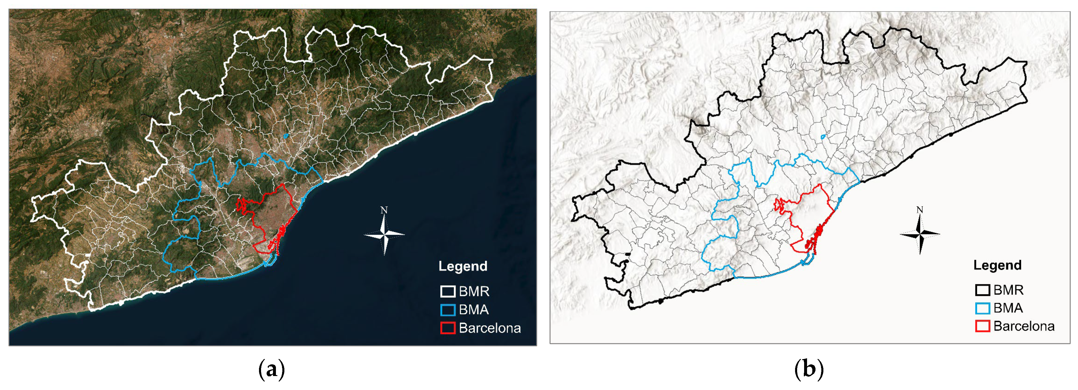
Figure 3.
Ecological environment quality assessment parameters of various types of land use in BMR during 2006-2018. (a) Ecological environment quality assessment parameters of various types of land use in BMR; (b) Main categories and overall ecological environment quality assessment parameters of BMR. *Note: The codes of various types of land use in Figure (a) correspond to Table 2.
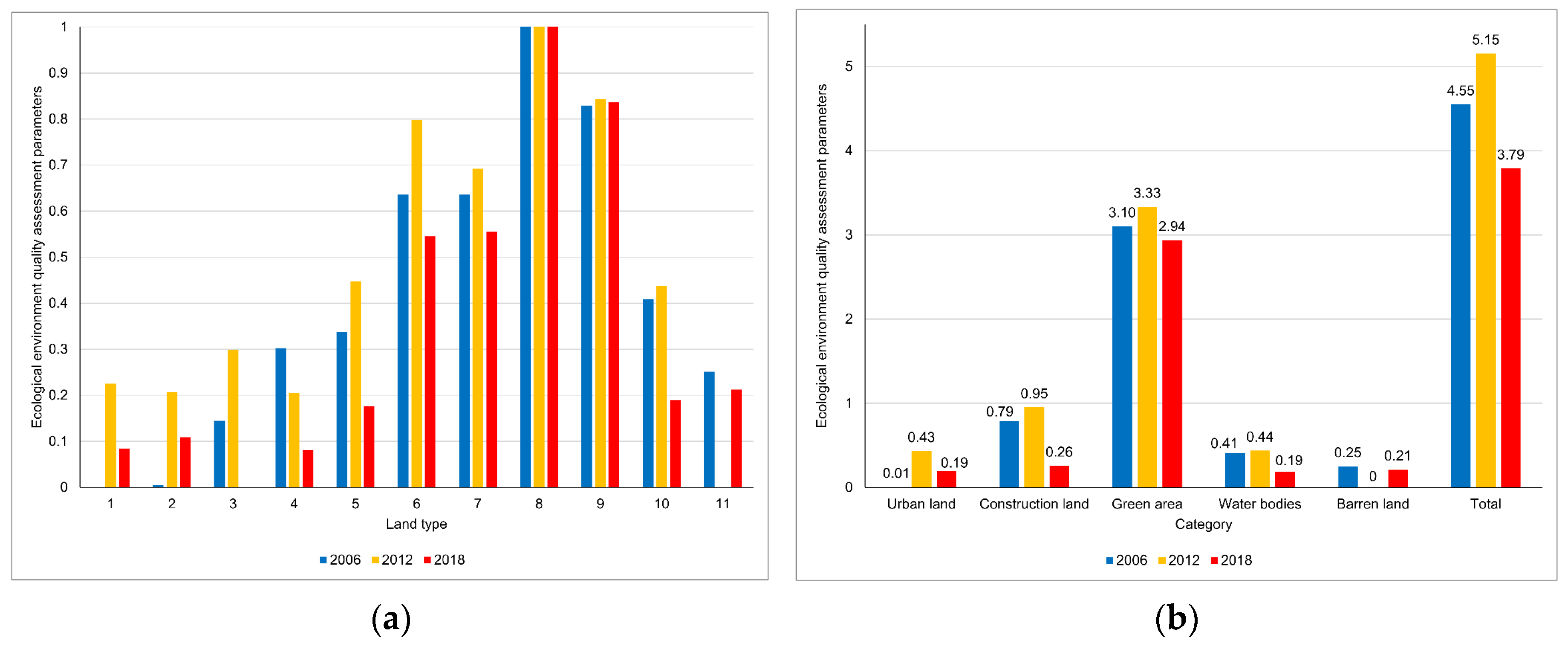
Figure 4.
Evolution of BMR green area distribution from 2006 to 2018.
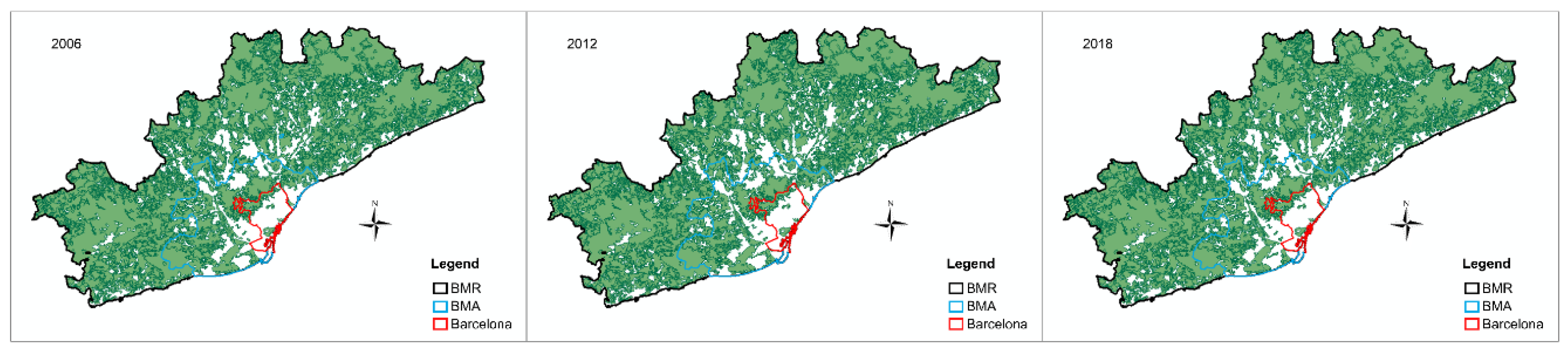
Figure 5.
Evolution of BMR green area and number of plaques from 2006 to 2018. (a) Evolution of BMR green area and proportion of BMR area; (b) number of BMR green plaques and proportion of plaques to green area.
Figure 5.
Evolution of BMR green area and number of plaques from 2006 to 2018. (a) Evolution of BMR green area and proportion of BMR area; (b) number of BMR green plaques and proportion of plaques to green area.
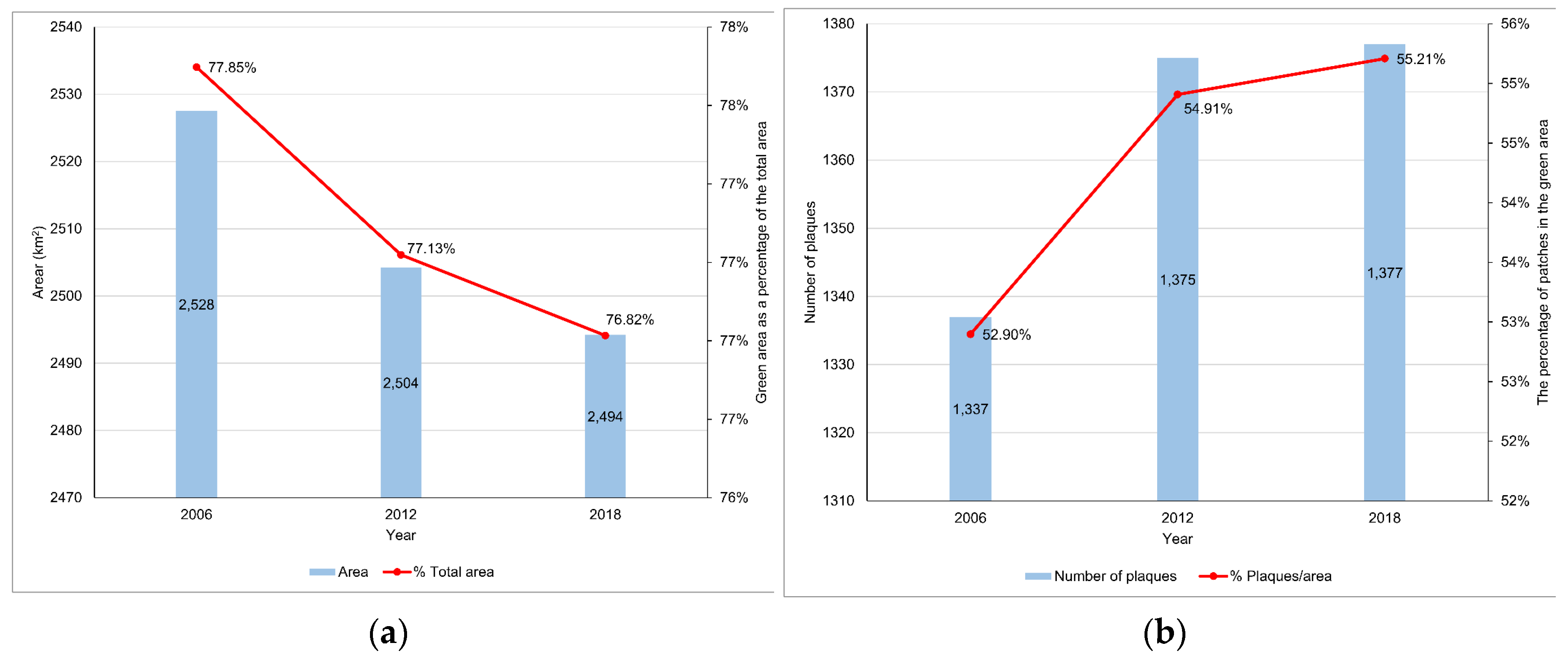
Figure 6.
EQI of various types of land use in BMR green areas from 2006 to 2018.
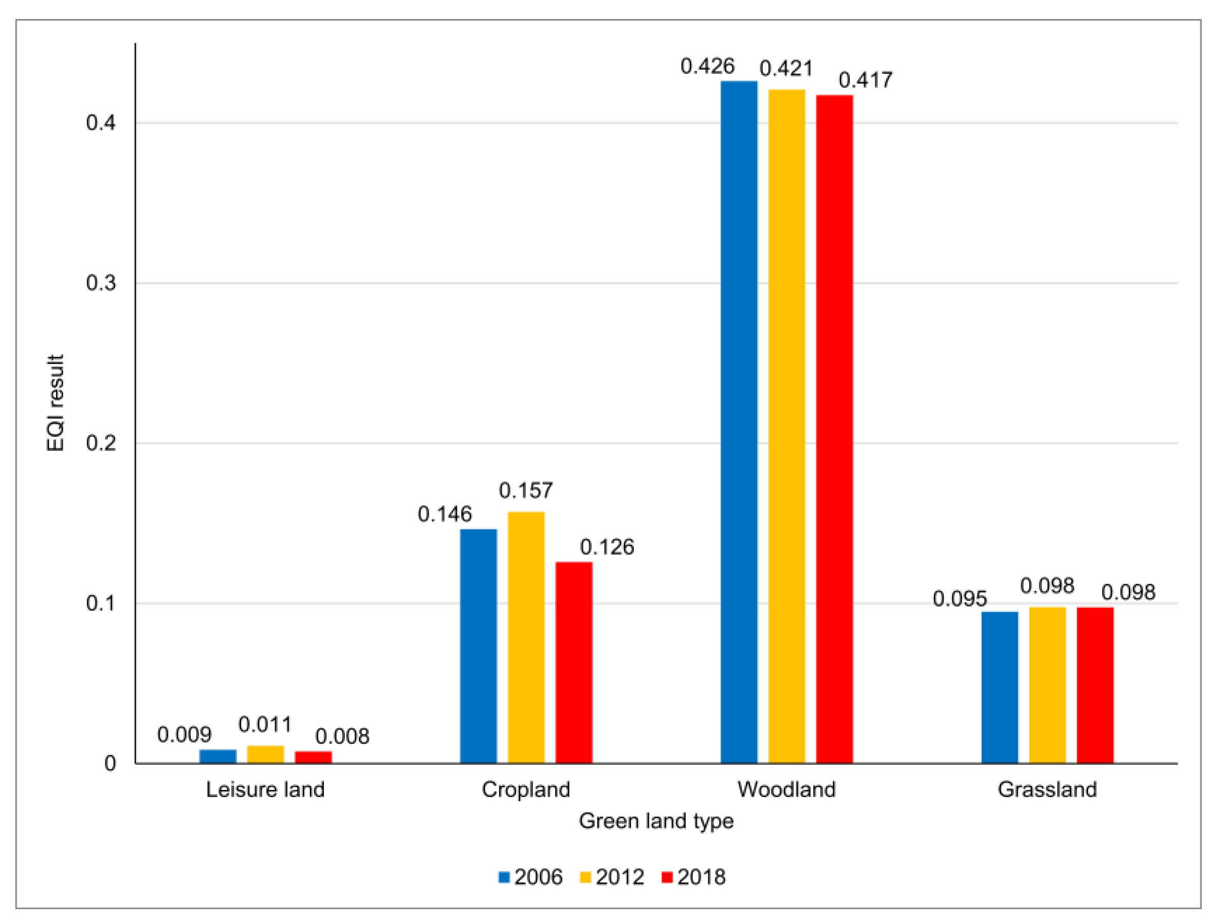
Figure 7.
Spatial distribution map of EQI assessment results in BMR from 2006 to 2018 (a, b and c). Spatial distribution map of EQI in BMR from 2006 to 2018; (d) Spatial variation in EQI in BMR.
Figure 7.
Spatial distribution map of EQI assessment results in BMR from 2006 to 2018 (a, b and c). Spatial distribution map of EQI in BMR from 2006 to 2018; (d) Spatial variation in EQI in BMR.
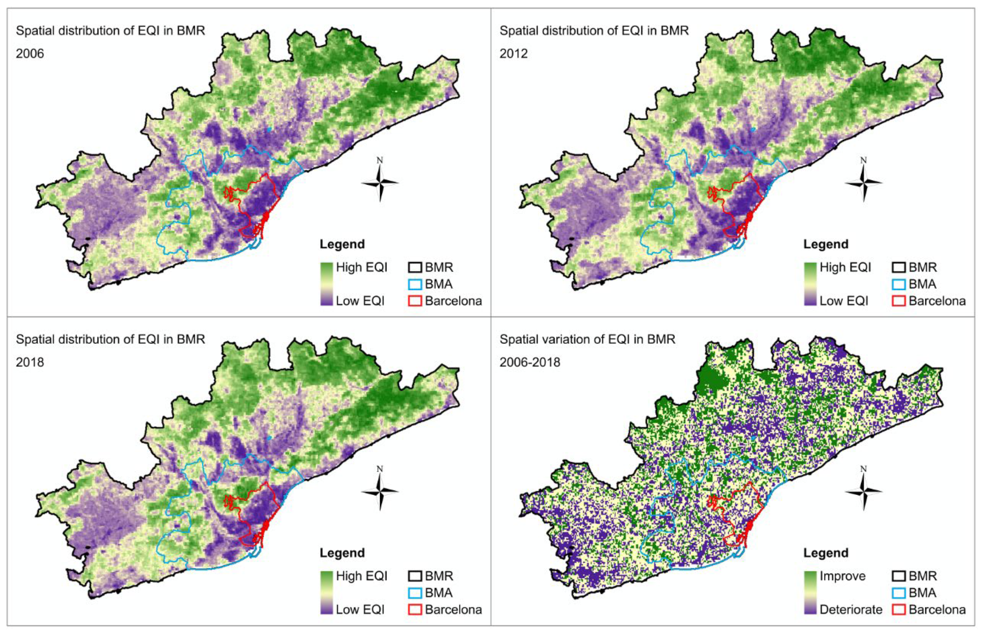
Figure 8.
Trends in the annual normalized statistical results of the average NDVI and climate factors of BMR from 2000 to 2023.
Figure 8.
Trends in the annual normalized statistical results of the average NDVI and climate factors of BMR from 2000 to 2023.
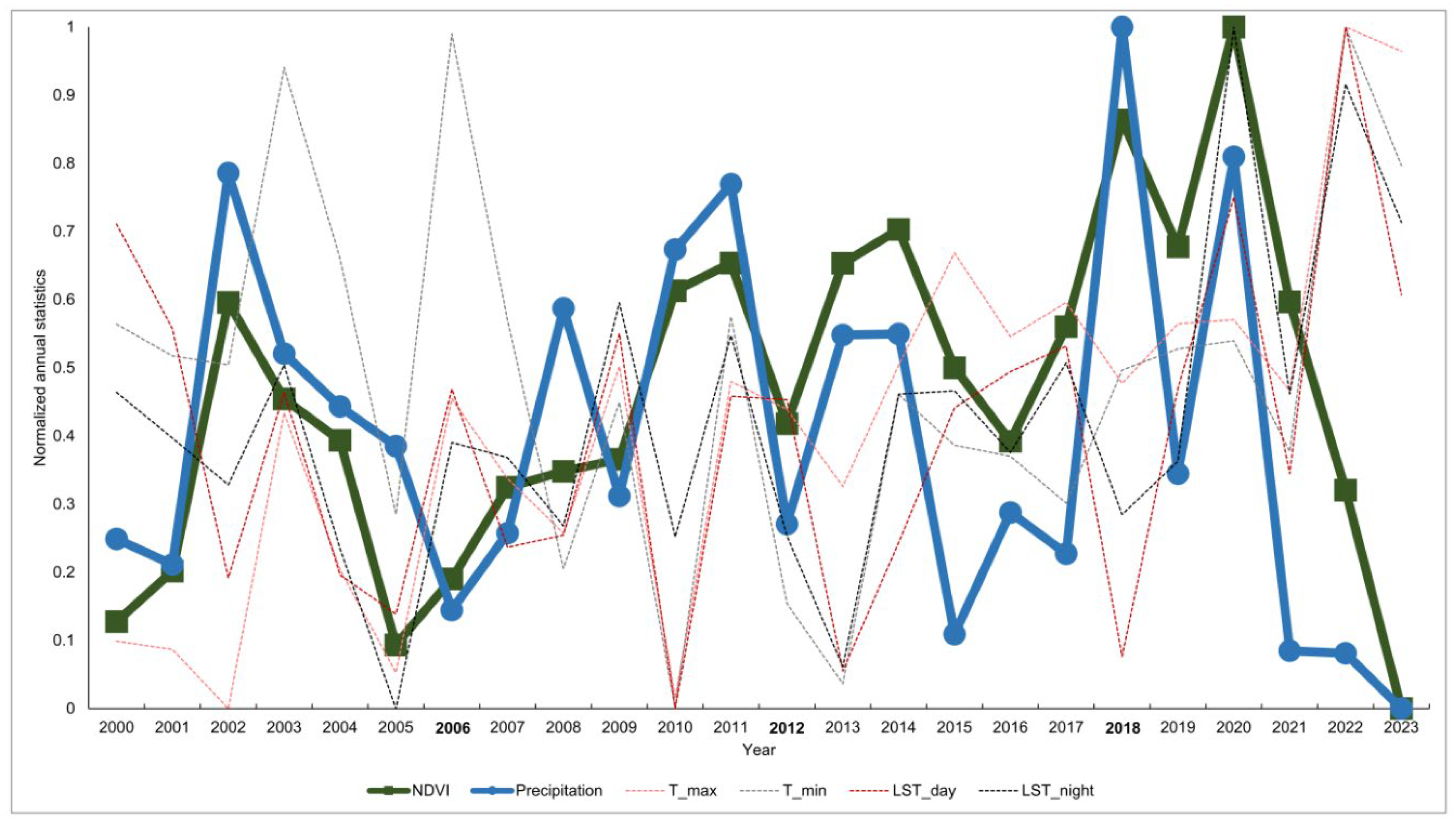
Figure 9.
The expected triangular spatial structure of the scatter plots of Ln(Mean_NDVI) and Ln(Mean_Precipitation) of BMR in 2006, 2012 and 2018.
Figure 9.
The expected triangular spatial structure of the scatter plots of Ln(Mean_NDVI) and Ln(Mean_Precipitation) of BMR in 2006, 2012 and 2018.
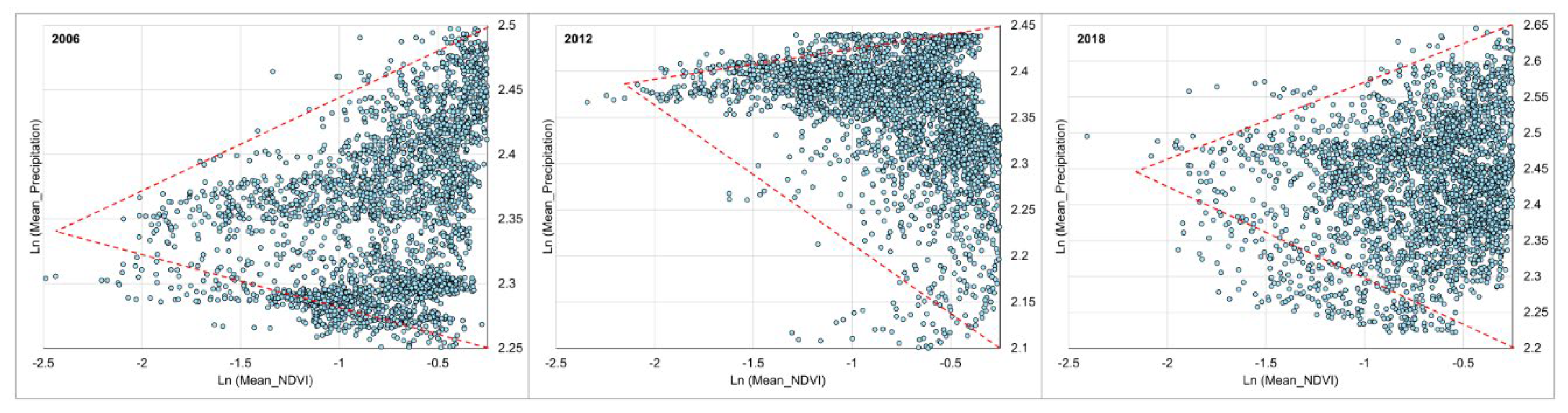
Figure 10.
Illustration of the triangular spatial characteristic structure of precipitation/NDVI scatter plot.
Figure 10.
Illustration of the triangular spatial characteristic structure of precipitation/NDVI scatter plot.
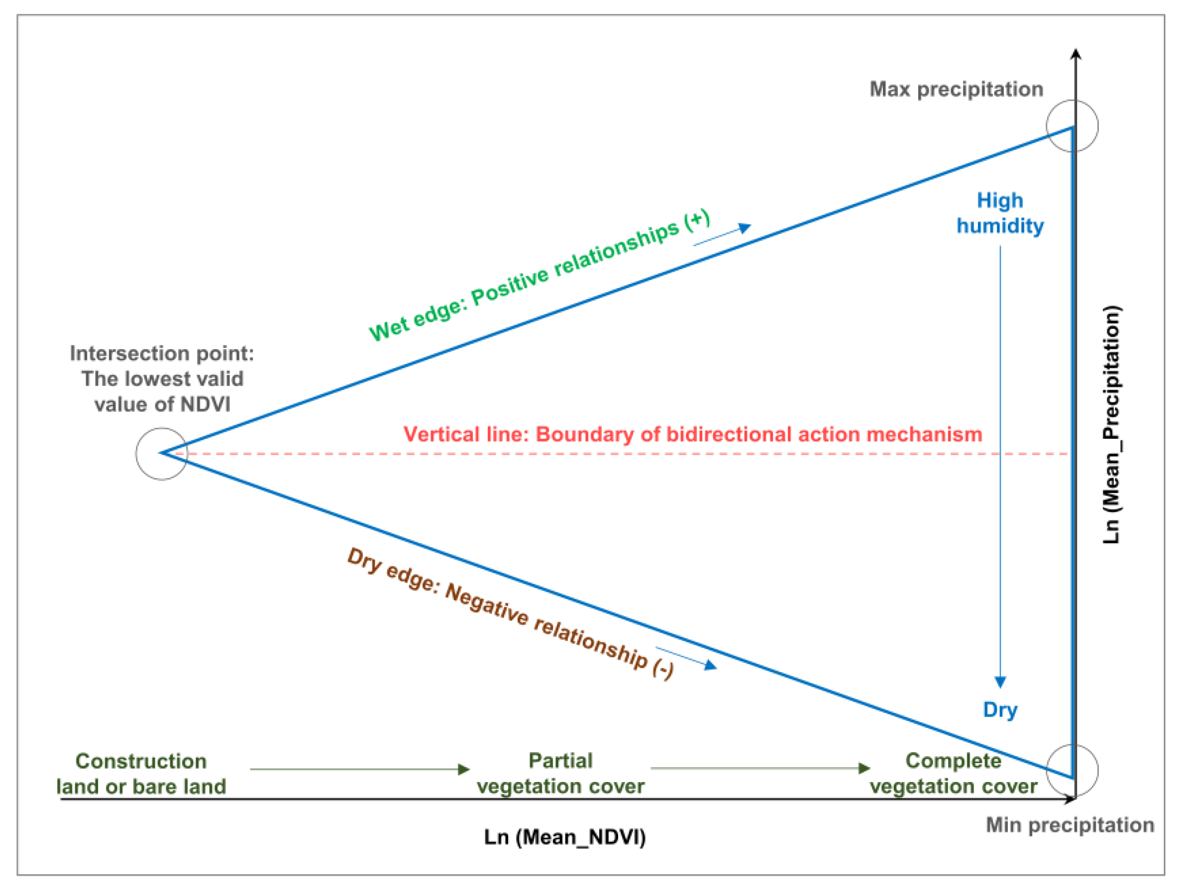
Figure 11.
Density distribution of precipitation/NDVI scatter points in BMR in 2006, 2012 and 2018.
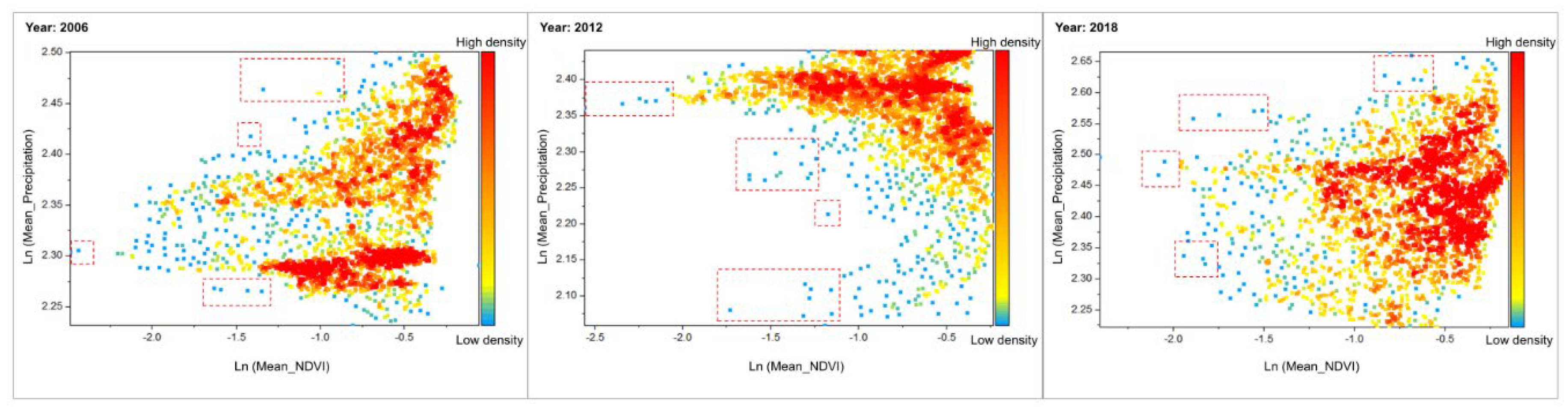
Figure 12.
Results of local anomaly detection of precipitation/NDVI in BMR in 2006, 2012 and 2018.
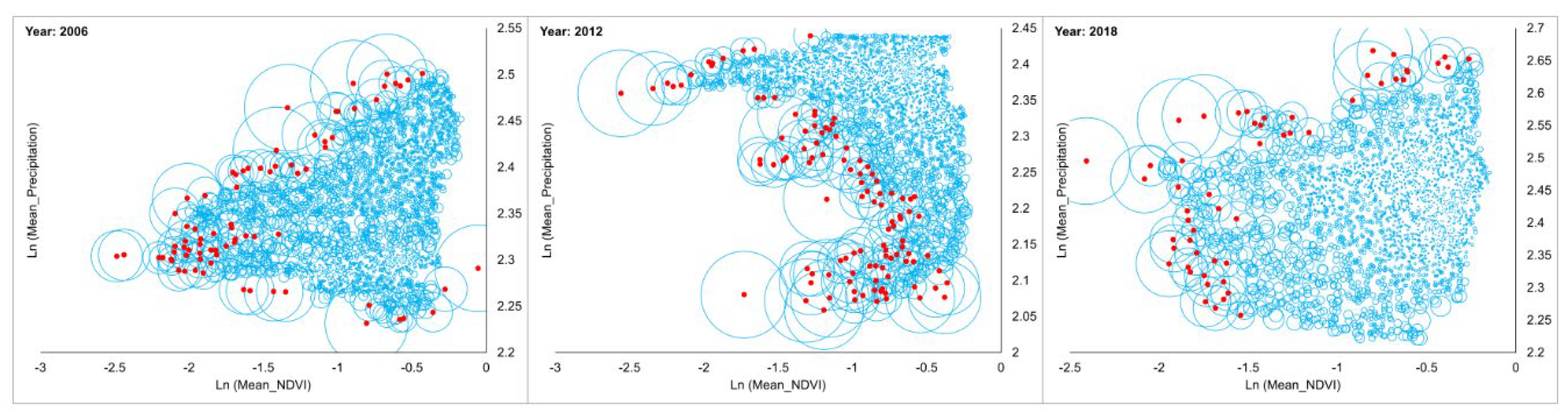
Figure 13.
Fitting equation of NDVI maximum precipitation between sub-regions in 2006 (example).
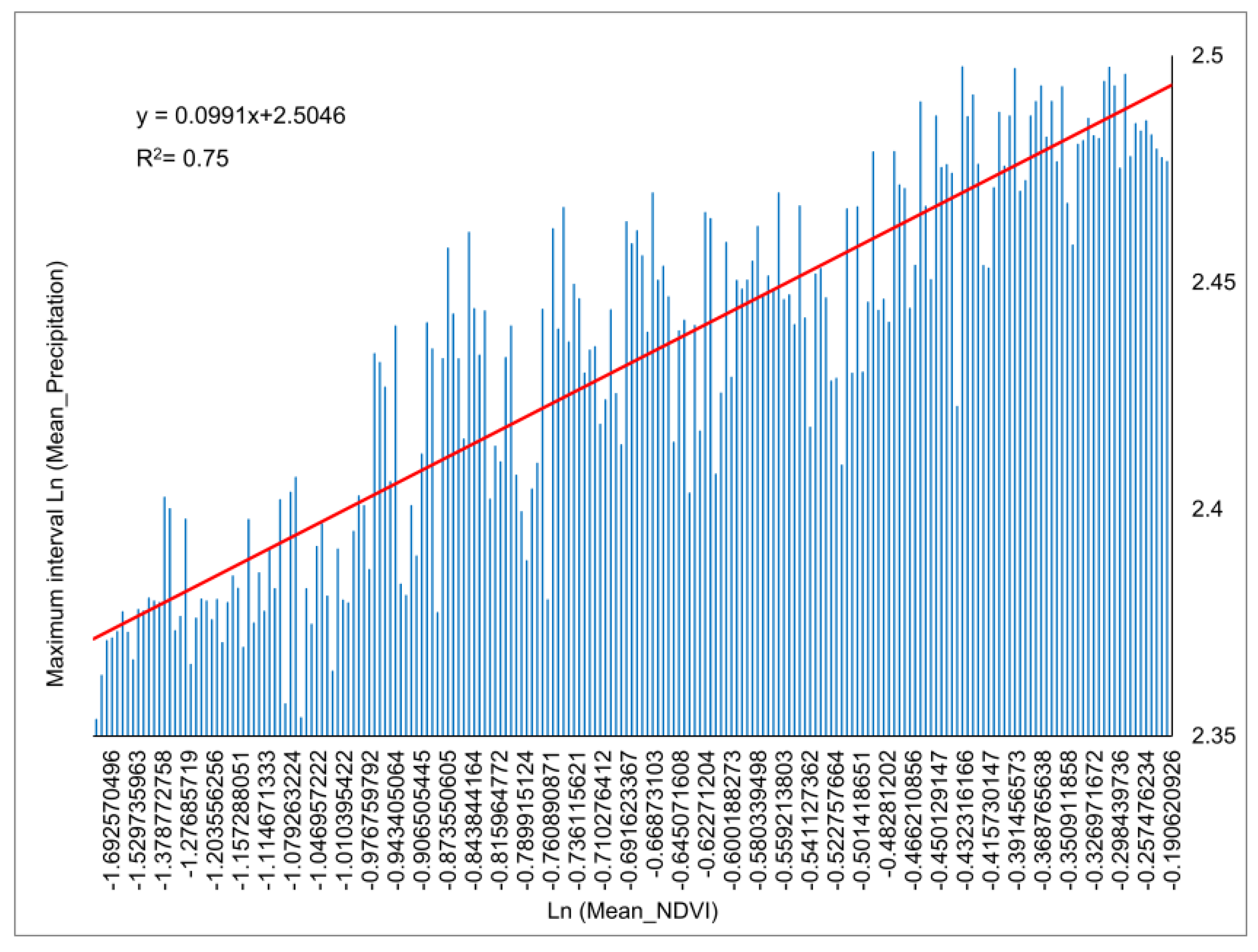
Figure 14.
Schematic diagram of the precipitation/NDVI characteristic triangle space of BMR in 2006, 2012 and 2018.
Figure 14.
Schematic diagram of the precipitation/NDVI characteristic triangle space of BMR in 2006, 2012 and 2018.
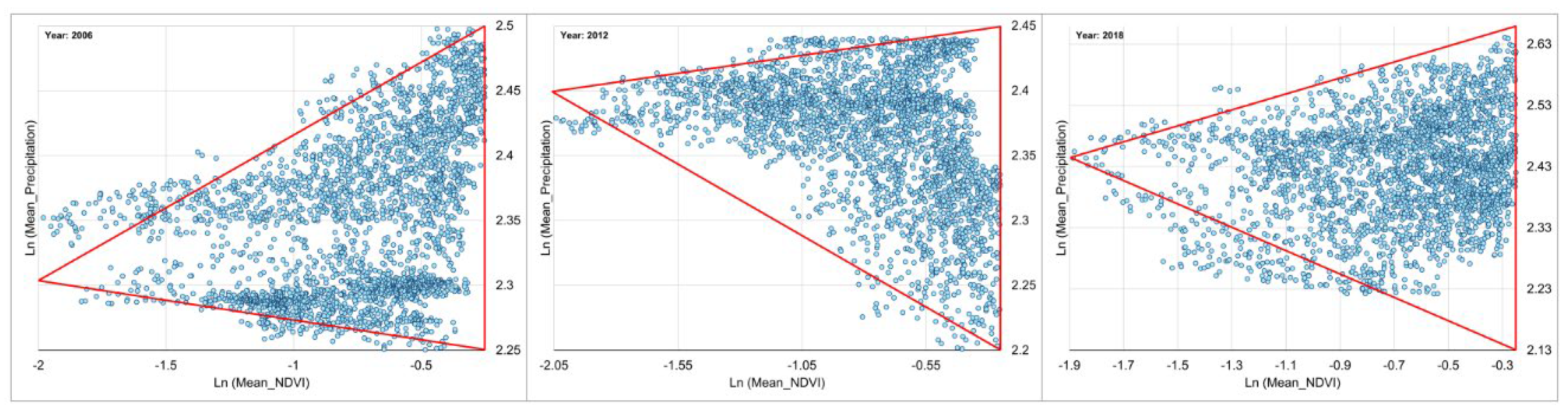
Figure 15.
Pixel distribution of each edge of the land cover & precipitation/NDVI characteristic triangle of BMR in 2006, 2012 and 2018.
Figure 15.
Pixel distribution of each edge of the land cover & precipitation/NDVI characteristic triangle of BMR in 2006, 2012 and 2018.
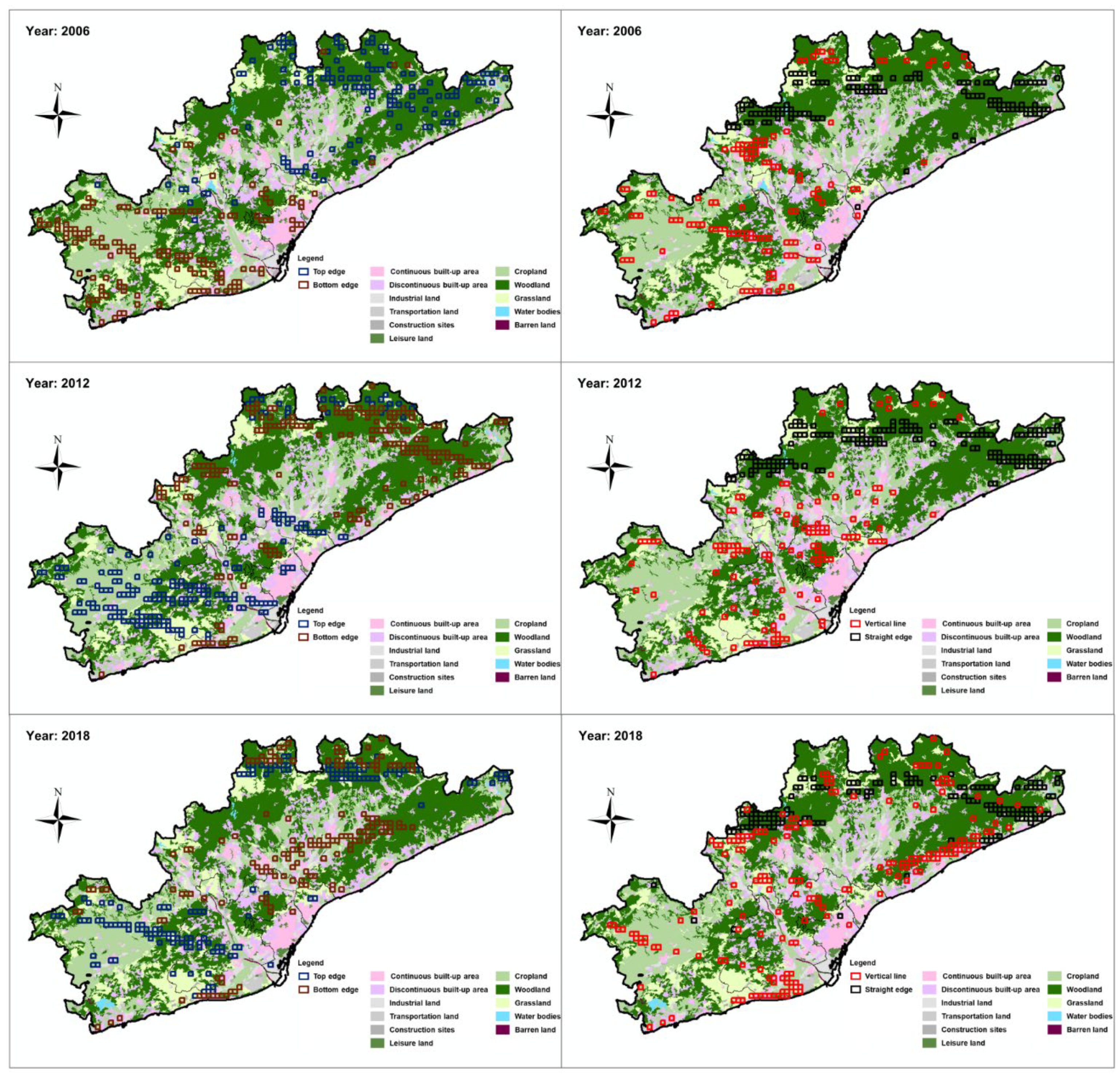
Table 1.
List of factors potentially influencing the key land use distribution.
| Type | Factors |
|---|---|
| Natural factors | Longitude |
| Latitude | |
| Distance from coastline | |
| Orientation | |
| Altitude | |
| NDVI | |
| Precipitation | |
| LST | |
| LST_day- LST_night | |
| T_max | |
| T_min | |
| T_max-T_min | |
| Human activity | NDBI |
| Urban heat island effect | |
| Impermeable area | |
| Artificial area | |
| Nighttime light data |
Table 2.
BMR land is reclassified and assigned to major categories*.
| Code | Reclassification | Categories |
|---|---|---|
| 1 | Continuous built-up area | Urban land |
| 2 | Discontinuous built-up area | |
| 3 | Industrial land | Construction land |
| 4 | Transportation land | |
| 5 | Construction sites | |
| 6 | Leisure land | Green area |
| 7 | Cropland | |
| 8 | Woodland | |
| 9 | Grassland | |
| 10 | Water bodies | Water bodies |
| 11 | Barren land | Barren land |
* A detailed description of the land uses included in each reclassification can be found in Appendix A.
Table 3.
BMR Ecological Environment Quality Index (EQI) evaluation results and the proportion of land use results of individual categories in the total results.
Table 3.
BMR Ecological Environment Quality Index (EQI) evaluation results and the proportion of land use results of individual categories in the total results.
| Categories | 2006 | 2012 | 2018 | |||
|---|---|---|---|---|---|---|
| EQI | % of total | EQI | % of total | EQI | % of total | |
| Urban land | 0.001 | 0.08% | 0.031 | 4.18% | 0.015 | 2.24% |
| Construction land | 0.013 | 1.88% | 0.021 | 2.88% | 0.002 | 0.32% |
| Green area | 0.676 | 97.73% | 0.687 | 92.77% | 0.648 | 97.25% |
| Water bodies | 0.002 | 0.24% | 0.001 | 0.17% | 0.001 | 0.14% |
| Barren land | 0.001 | 0.07% | 0.000 | 0 | 0.0003 | 0.05% |
| Overall | 0.692 | 100.00% | 0.740 | 100.00% | 0.667 | 100.00% |
Table 4.
Green area proportion OLS models.
| Independent variable b | Model_2006 a | Model_2012 a | Model_2018 a | |||||||||
|---|---|---|---|---|---|---|---|---|---|---|---|---|
| B | Beta | t | Sig. | B | Beta | t | Sig. | B | Beta | t | Sig. | |
| Constant | -1719.33 | -6.00 | 0.00 | -1534.85 | -4.79 | 0.00 | -2681.47 | -5.75 | 0.00 | |||
| Longitude | 0.00 | -0.17 | -7.02 | 0.00 | 0.00 | -0.12 | -4.26 | 0.00 | 0.00 | -0.16 | -3.86 | 0.00 |
| Latitude | 0.00 | 0.19 | 5.41 | 0.00 | 0.00 | 0.17 | 4.92 | 0.00 | 0.00 | 0.31 | 5.49 | 0.00 |
| Distance from coastline | 0.00 | -0.13 | -5.65 | 0.00 | 0.00 | -0.08 | -4.31 | 0.00 | 0.00 | -0.06 | -2.13 | 0.03 |
| Orientation | 0.00 | 0.00 | -0.13 | 0.89 | 0.00 | 0.00 | -0.76 | 0.45 | 0.00 | 0.00 | -0.74 | 0.46 |
| Altitude | 0.00 | -0.02 | -2.13 | 0.03 | 0.00 | 0.00 | 0.33 | 0.74 | 0.00 | 0.00 | 0.18 | 0.86 |
| Slope | 2.78 | 0.04 | 8.59 | 0.00 | 0.29 | 0.00 | 0.54 | 0.59 | 1.61 | 0.02 | 4.22 | 0.00 |
|
NDVI_ MEAN |
6.77 | 0.00 | 0.25 | 0.80 | 5.98 | 0.03 | 1.89 | 0.06 | 5.45 | 0.03 | 1.73 | 0.08 |
| Precipitation | 1.21 | 0.03 | 1.42 | 0.16 | 0.97 | 0.02 | 2.13 | 0.03 | 0.93 | 0.03 | 3.89 | 0.00 |
| LST_DAY- LST_NIGHT |
0.22 | 0.02 | 2.01 | 0.04 | -0.12 | -0.01 | -0.82 | 0.41 | 0.18 | 0.01 | 1.30 | 0.20 |
| T_max | 0.50 | 0.01 | 1.38 | 0.17 | 0.83 | 0.02 | 1.53 | 0.13 | 4.03 | 0.14 | 8.05 | 0.00 |
| T_max-T_min | -1.03 | -0.03 | -3.18 | 0.00 | -0.76 | -0.03 | -1.95 | 0.05 | -3.55 | -0.09 | -7.83 | 0.00 |
| NDBI | -1.90 | -0.01 | -0.87 | 0.38 | -1.92 | 0.02 | 1.61 | 0.11 | -1.00 | 0.02 | 1.16 | 0.25 |
| UHIE_ NIGHT |
-0.02 | 0.00 | -0.13 | 0.90 | 0.65 | 0.03 | 2.28 | 0.02 | -0.27 | -0.01 | -1.08 | 0.28 |
| Impermeable area | -15.53 | -0.15 | -12.84 | 0.00 | -25.96 | -0.25 | -17.79 | 0.00 | -15.74 | -0.15 | -10.93 | 0.00 |
| Artificial area | -80.61 | -0.83 | -64.97 | 0.00 | -72.64 | -0.75 | -49.37 | 0.00 | -81.32 | -0.83 | -56.55 | 0.00 |
| Night Light | -0.03 | -0.02 | -2.55 | 0.01 | -0.02 | -0.01 | -1.33 | 0.19 | 0.01 | 0.00 | 0.50 | 0.62 |
a The dependent variable of the three models is the proportion of green area in that year. b LST_DAY, LST_NIGHT, T_min and UHIE_DAY became excluded independent variables during the regression analysis.
Table 5.
Multiple OLS models between mean NDVI and various climate factors a.
| Independent variable | R2 | B | Beta | t | Sig. |
|---|---|---|---|---|---|
| Precipitation | 0.47 | 0.00 | 0.68 | 4.40 | 0.00 |
| T_max | 0.00 | 0.00 | 0.05 | 0.25 | 0.81 |
| T_min | 0.08 | -0.01 | -0.28 | -1.39 | 0.18 |
| LST_day | 0.06 | 0.00 | -0.24 | -1.14 | 0.27 |
| LST_night | 0.02 | 0.00 | 0.13 | 0.62 | 0.54 |
a The dependent variable for all models is the annual mean NDVI.
Table 6.
The spatial three-side fitting results of the precipitation/NDVI characteristic triangle of BMR in 2006, 2012 and 2018.
Table 6.
The spatial three-side fitting results of the precipitation/NDVI characteristic triangle of BMR in 2006, 2012 and 2018.
| Year | Top edge | R2 | Bottom edge | R2 | Straight edge |
|---|---|---|---|---|---|
| 2006 | y=0.0991x+2.5046 | 0.7510288 | y=-0.0258x+2.2563 | 0.1790952 | x=-0.1705 |
| 2012 | y=0.0261x+2.4428 | 0.2359837 | y=-0.0841x+2.2153 | 0.5709729 | x=-0.2341 |
| 2018 | y=0.113x+2.6567 | 0.375945 | y=-0.1641x+2.1339 | 0.6198449 | x=-0.3823 |
Table 7.
Summary of parameters of the spatial structure of precipitation/NDVI characteristic triangles in BMR in 2006, 2012 and 2018 a.
Table 7.
Summary of parameters of the spatial structure of precipitation/NDVI characteristic triangles in BMR in 2006, 2012 and 2018 a.
| Year | 2006 | 2012 | 2018 | |||
|---|---|---|---|---|---|---|
| Max Precipitation | 2.49 | (12.01) | 2.44 | (11.43) | 2.64 | (14.00) |
| Min Precipitation | 2.26 | (9.59) | 2.24 | (9.35) | 2.16 | (8.67) |
| Intersection point_Precipitation | 2.31 | (10.05) | 2.39 | (10.90) | 2.44 | (11.51) |
| Intersection point_Min NDVI | -1.99 | (0.14) | -2.06 | (0.13) | -1.89 | (0.15) |
| Max NDVI | -0.19 | (0.83) | -0.24 | (0.79) | -0.16 | (0.85) |
| Straight edge length | 0.22 | 0.20 | 0.48 | |||
| Wet edge slope | 0.10 | 0.03 | 0.11 | |||
| Dry edge slope | -0.03 | -0.08 | -0.16 | |||
| Top triangle area | 0.16 | 0.04 | 0.17 | |||
| Bottom triangle area | 0.04 | 0.14 | 0.24 | |||
| Total area | 0.20 | 0.18 | 0.41 | |||
a The original value of the parameter is shown in brackets.
Disclaimer/Publisher’s Note: The statements, opinions and data contained in all publications are solely those of the individual author(s) and contributor(s) and not of MDPI and/or the editor(s). MDPI and/or the editor(s) disclaim responsibility for any injury to people or property resulting from any ideas, methods, instructions or products referred to in the content. |
© 2024 by the authors. Licensee MDPI, Basel, Switzerland. This article is an open access article distributed under the terms and conditions of the Creative Commons Attribution (CC BY) license (http://creativecommons.org/licenses/by/4.0/).
Copyright: This open access article is published under a Creative Commons CC BY 4.0 license, which permit the free download, distribution, and reuse, provided that the author and preprint are cited in any reuse.


