
Submitted:
11 November 2024
Posted:
12 November 2024
You are already at the latest version
Abstract
Strong motion records from full-scale structures provide the ultimate evidence of how real structures, in situ, respond to earthquakes. The most effective method for visualizing the recorded response is by animation. This paper presents a novel method for visualization of the motion of a building that is densely instrumented with triaxial accelerometers and rotational seismometers. The method is based on one- and two-dimensional biharmonic spline interpolation of the motion between multiple sensors on a floor or along the building height. It is demonstrated on a 50-story skyscraper uniquely instrumented with multiple triaxial accelerometers per floor, approximately at every five floors above ground and at two basement levels, and two borehole arrays measuring the motion of the soil very near the building foundation. The animations provide valuable insight into the three-dimensional structural response, including wave propagation through the structure and the interplay between translations and rotations, which will be useful for testing existing and developing new methods for structural health monitoring of buildings and for the further development of building design codes. Animations of selected earthquakes can be found on YouTube at @TPYC-seismic.
Keywords:
dynamic surface deformation
; biharmonic spline interpolation
; visualization of observed earthquake response of buildings
; animation of building response recorded by 3DOF and 6DOF sensors
; densely instrumented buildings
; Tongde Plaza Yue Center (TPYC) testbed structure
1. Introduction
We present a new method for visualizing, in space and in time, observed three-dimensional (3D) motion of a densely instrumented building, with an application to earthquake response recorded in a 50-story skyscraper (Figure 1) [1]. The method involves representation of the floor slab motion as a dynamic surface deformation defined by a two-dimensional (2D) biharmonic spline [2,3,4,5,6,7,8], with parameters determined from recorded motions by multiple triaxial accelerometers on that floor and additional constraints obtained from motions recorded at other floors. The method can be extended to other types of densely instrumented structures, like bridges and dams.
Earthquake records from instrumented structures have been essential for the evolution of earthquake engineering; a review of the progress in the sensor technologies and deployment since the 1930s can be found in [9]. The first comprehensive set of earthquake records in structures were generated by the San Fernando, California earthquake of 1971 and presented visually in terms of plots of time histories of recorded acceleration, velocity and displacement of the individual records and the corresponding Fourier and response spectra [10]. Such form of visual presentation has become the standard and is currently disseminated over the internet [11,12,13,14]. To maximize the coverage of different types of construction in different seismic zones, the strong motion arrays in buildings have been sparse, with only few instrumented floors and with uniaxial or biaxial accelerometers recording only horizontal response. Methods have been proposed to reconstruct the motion at the non-instrumented floors directly by interpolation [6,7,8], a model of the structure [15,16] or a combination of the two [17,18]. The number of densely instrumented buildings has been slowly but steadily growing [19,20,21,22,23,24,25,26,27,28,29]. Yet, even in these buildings, only the horizontal components of the floor responses are recorded, while vertical motions are typically recorded only in the basement.
Rare examples of densely instrumented buildings with sensors recording vertical floor motion are the Los Angeles 52-story building, instrumented with one triaxial accelerometer at practically every floor [25] and the case study in this paper, a 50-story building, with instrumented approximately every fifth floor above ground, but by multiple triaxial accelerometers, and two basement levels instrumented each with 7 triaxial accelerometers, which enables reconstruction of the motion of the floor slabs [1]. Analyses of vertical vibrations recorded in these two buildings can be found in [30,31].
The case study in this paper is also a rare example of a full-scale building permanently instrumented with rotational seismometers. One of them is in the basement and the other one is on the 48th floor (Figure 1), the latter being used to reconstruct the 48th floor slab motion, as shown in the next section. Recent articles on rotational sensors and their applications to recording ground motion and structural response can be found in [28,29,30,31,32,33]. An analysis of earthquake records of rotations recorded in the 50-story case study can be found in [34]. Finally, unique elements of the sensor array in the case study are two borehole arrays installed close to the building, with one sensor at the ground surface and another at the depth reached by the piles (~50 m), the motions of which are also animated.
At the core of the proposed visualization methodology is biharmonic spline interpolation, which is particularly effective in reconstructing smooth, continuous surfaces from sparse and irregularly spaced data points. It has been previously applied, e.g., to interpolation of satellite altimeter data [2], surface reconstruction in computer graphics [3], solar radiation mapping [5] and reconstruction of horizontal floor motion in sparsely instrumented buildings [6,7,8].
In this paper, it is used to reconstruct the floor slab motion, separately for each component of motion, at a sequence of time instants, creating an animation. To the knowledge of the authors, this is the first case of visualization of floor deformations of buildings during an earthquake directly from observed data, not involving a model of the structure, and the first visualization of 3D response of a building directly from recorded response.
This paper is organized as follows. Section 2 presents a brief summary of the case study, the data and the methodology. The theoretical background of biharmonic spline interpolation for observations distributed spatially in 1D and 2D is reviewed and the specific steps of the application to the case study are deliberated. Section 3 presents the results in the form of snapshots of an animation for an earthquake and a pointer to a YouTube channel where animations can be viewed for several earthquakes. Finally, Section 4 presents the conclusions of this study.
2. Materials and Methods
2.1. Building and Data
The building is known as Tongde Plaza Yue Center (TPYC) and is located in Kunming, Yunnan Province of China. It is a reinforced concrete (RC) construction, with 50 floors (238 m) above and 4 floors (17.8 m) below ground (Figure 1 and Figure 2), comprising a tower and a basement proper encompassing the tower below ground. The tower is 70.8×29 m2 in plan, approximately symmetrical in both horizontal directions, while the basement is 105.6×58.9 m2 in plan and 17 m deep. They are both supported by a raft foundation and 30 m long RC friction piles. The building use is commercial, and the basement is used for parking. Figure 1 shows the East and South elevations and Figure 2 shows typical floor layouts of the floors above ground (parts (a) to (d)) and of basements -B1 and -B4 (parts (e) and (f)). Figure 3 shows the distribution of mass and lateral stiffness along the height in the Nort-South (NS) and East-West (EW) directions; the latter was obtained from a detailed finite element model of the tower, fixed at the ground floor [30]. It can be seen that the tower is stiff near the base and flexible near the top.
Since January of 2021, more than 35 earthquakes were recorded in the building, with epicenters in Yunnan and Sichuan Provinces of China and neighboring Burma, Laos and India, magnitudes , epicentral distances between 10 and 1,008 km and focal depts between 9 and 128 km. The largest motions were recorded during M6.4 Yangbi, Dali, Yunnan earthquake of May 21, 2021, and M6.8 Kanding, Garze, Sichuan earthquake of September 5, 2022. The peak ground horizontal and vertical accelerations recorded on the ground surface near the South-East corner of the basement were 1.84×10⁻³ g and 1.02×10⁻³ g (Yangbi), and 1.30×10⁻³ g and 0.68×10⁻³ g (Kanding); 1g = 9.80665 m/s². The earthquakes caused small response, within 9×10⁻³ g at the 48th floor, and no damage. More details about the structure, soil, structural health monitoring system and recorded earthquakes can be found in [1,39,306].
The instrumentation includes 26 triaxial accelerometers distributed across eleven levels of the tower, located at floors 1F, 5F, 10F, 16F, 21F, 26F, 31F, 36F, 42F, 48F, and 50F. Additionally, fourteen triaxial accelerometers are installed at two basement levels (−1B and −4B). The two borehole arrays are equipped each with two accelerometers, one at the surface and the other one at 48.4 m depth. Complementing the accelerometer array are two rotational seismometers situated at −4B and 48F and a weather receiver located on Roof 4. The sensor layout can be seen in Figure 1 and Figure 2.
All accelerometers are Class B Micro-Electro-Mechanical Systems (MEMS) servo silicon sensors (EQR120) [1]. Those in the tower and basement have recording range of ±3g and a threshold sensitivity of 2.4×10⁻⁶ g while those of the borehole arrays have recording range of ±5g with a threshold of 3.9×10⁻⁶ g. The rotational seismometers are R2 angular velocity meters, with resolution 6×10⁻⁸ rad/s at 1 Hz [30,38]. Data acquisition is performed at a sampling frequency of 200 Hz, corresponding to a Nyquist frequency of 100 Hz.
Figure 4 shows a schematic representation of the sensor locations, relative to the slabs of the instrumented levels, which is used to create the animations. On the left, a side view is shown and, on the right, a bird’s view. The locations of the sensors in the basement can be seen more clearly in Figure 2. Table 1 shows the coordinates of the sensor locations relative to the coordinate system, described in more detail in the next section. Figure 5 shows the convention for the six degrees of freedom motion (6DOF) recorded by collocated accelerometer and R2 rotational seismometer.
2.2. Slab Motion Representation by 2D Biharmonic Splines Using Data from Triaxial Sensors
Historically, the term "spline" referred to flexible strips used by draftsmen to draw smooth curves between points. Biharmonic splines represent an extension of this concept to higher dimensions and are valuable in applications where data may be sparse or noisy, and a smooth approximation is desired [2,3]. In one and two dimensions, the biharmonic splines are cubic polynomials that have minimum curvature and continuous first and second derivatives. It has been shown that, in all dimensions, the biharmonic splines have minimum curvature satisfying the constraints [40].
The motion of the building is described relative to a global reference coordinate system , with origin at the center of the first floor, the and axes pointing East and North and the -axis pointing upward. Let be local coordinate systems with origin at a particular floor that is at elevation from the ground surface (Figure 4). Then, in the global coordinate system, the points on the slab have coordinates , and . Both coordinate systems are fixed and are defined relative to the position of the building at rest. Let be a position vector describing the location of an arbitrary point on the slab in the local coordinate system and let be a three-dimensional vector describing the displacement of that point at time relative to its position at rest. We wish to express at an arbitrary time instant as a smooth function of the spatial coordinates such that satisfies the constrains that at a given set of points on the slab, it has values
Assuming small displacements, we represent each component individually as a biharmonic spline satisfying the corresponding component of the constraints.
Let be any one of the components of at time and let be its constraints. Then, must satisfy the biharmonic equation and the constraints
in which is the biharmonic operator and is the Dirac delta function (Sandwell, 1997). The solution can be represented as a linear combination of the Green’s functions of the biharmonic operator
The Green’s functions are impulse response functions of the operator and satisfy
In two dimensions [2]
Both and its gradient are continuous everywhere, including at . The unknown coefficients can be obtained by substituting into the constraints the representation of from Eqn (3), which leads to a linear system of equations
The system of equations in (6) can be written in matrix form as
in which has entries , and , and is solved for . The system has a stable solution if no two rows or columns of are the same, which requires that the points are well distributed on the slab. In case of many available measurement points that are “noisy”, it is desirable to reduce the order of the system using singular value decomposition.
The Green’s functions matrix is the same for all three components of motion and does not depend on time. So, it is precomputed and used repeatedly. After the coefficients for all three degrees of freedom, , and , have been computed at a time instance , the displacement components are computed at that instance on a dense grid of uniformly spaced points on the slab,
Then, the position of the points on the grid at time in the absolute coordinate system is computed
plots of which show how the slab deforms in time during the earthquake shaking.
2.3. Slab Motion Representation by a Plane Using Data from 6DOF Sensor
At the 48th floor, the motion was recorded by a 6DOF sensor (collocated accelerometer and R2 rotational seismometer), located at the center of the floor, i.e., at the origin of the local coordinate system. In the local coordinate system, the position of the points on the slab is defined by vector . Let and be the displacements and angles of rotation recorded at the origin, . Then, the slab motion can be represented by a plane that translates and rotates.
The displaced position of points on the plane can be computed by adding to the translation at , , displacements resulting from a sequence of rotations about the -, - and -axes. The latter are linear transformations represented respectively by rotation matrices
Then, the position of the points on the slab at time in the local coordinate system are
2.4. Estimating Additional Constraints from 3D Motions Recorded by Sensors at Other Floors
The accuracy and stability of biharmonic spline interpolation in representing the slab deformation depend on the number of the measurement points and their spatial distribution. The number of measurements in our case study, however, is limited to two or three in the tower above ground and to 7 in the basement, and, at the 48th floor, there is only one 6DOF measurement at the center. Consequently, to ensure realistic displacements of the slabs at the unconstrained corners, we attempt to create additional constraints, based on information from the triaxial accelerometers at the same or other floors and the fitted plane at the 48th floor (see section 2.3) and considering the fact that the displacements from the slab deformations are relatively small compared to the overall deformation of the building.
For the floors with three sensors, two of which are at the opposite corners of one of the diagonals (see Figure 6), we construct constrains at the corners of the other diagonal using the measurements at the same floor, as follows. Let and be the positions of the existing sensors and and be their displacements at time . Then the midpoint position and displacement are
Assuming small rotations and displacements, the rotational angles at , , , and , can be approximated using finite differences as [41]
which enables construction of the rotation matrices , , and , defined in Eqns (10) to (12), and the combined rotation matrix
Then, the motions at the non-instrumented corners, at , , can be estimated as
providing additional constraints in Eqn (1).
For floors with two sensors, we construct additional constraints using measurements at the other floors along the same vertical, using 1D spline interpolation, as follows. Let represent any one of the displacement components (, , or ) as a function of elevation , with known values , . The biharmonic equation in one dimension and the associated constraints can be written as [2]
and has solution that is a linear combination of the 1D biharmonic operator Green's functions
in which
Then, the displacement at another height along the vertical, where there is no sensor, can be estimated by solving the linear system of equations
By applying this approach to each displacement component, we estimate the displacements at the non-instrumented corners providing additional constraints for the representation of the slab motion at the floors with two sensors.
At the 48th floor, where measurement of 6DOF motion is available but only at one point, we showed in section 2.3 how the slab motion can be approximated by a translating and rotating in time plane. The motion of the slab can also be approximated by a 2D spline interpolation, by using the plane to construct constraints at the four corners (Figure 6). Then, a biharmonic spline can be fitted though the five points, representing a more natural slab displacement for the visualization.
It is noted that, using 1D spline interpolation along vertical lines, where motion is measured at some levels, the motion at the non-instrumented floors can be reconstructed, and can then be used for rapid assessment of the structural health during or immediately after the end of the shaking.
2.5. Steps
First, the data are prepared. The displacements are computed by double integration of the recorded accelerations and the angles of rotation are computed by integration of the recorded angular velocities, after performing instrument correction with manufacturer provided sensor specific transfer-functions. Then, the data is high pass filtered, to remove low frequency noise, low pass filtered at 10 Hz and subsampled by a factor of 6 to reduce the computation time to generate the animation. This results in an animation with about 33 frames per second.
Then, the visualization is created according to the following steps, each one consisting of adding a particular element to the animation. The first four steps are illustrated in parts a) to d) of Figure 7.
Step 1: Add the slabs at levels F48, F42, F36, F31, F21, F26, F16, F10, F5, F1, B1, and B4, which have been sufficiently instrumented to reconstruct the slab motion. The slab motion is defined at a 1×1 m2 grid of points.
Step 2: Add the physical boundaries of the structure, represented by vertical lines, to facilitate the visualization of the sensor placements relative to the physical layout.
Step 3: Add the locations of the sensors. The locations of the accelerometers are marked as red dots and those where 6DOF motion is recorded are marked by blue dots. The motion of these points is added as a check for the reconstructed motions and to show the particle motions at locations at which no interpolation was applied (at F51 and at the borehole arrays).
Step 4: Add lines connecting sensors on neighboring floors and add labels indicating the level.
Step 5: Construct hodograms showing the particle motion of the soil recorded by the borehole sensors at the surface (SURF-NW and SURF-SE) and at depth (BOR-NW and BOR-SE). The particle motions are shown in the vertical plane passing through the radial direction, relative to the earthquake epicenter. The purpose of these plots is to visualize the particle motion during the passage of Rayleigh waves. Figure 8 shows an example of a hodogram at a particular instant of time. The thick fading line shows the trajectory of the particle motion during the past 2 s, with the color fading in the direction of the past.
Step 6: Construct a plot of time histories of the , and components of the displacement at the center of the 4th basement (-B4C5), with a slider showing the current time in the animation. This plot illustrates the entire time history of the effective input motion into the building and the current stage of the animation.
Step 7: Choose the magnification factor for the displacements to enable viewing the features of small amplitude response. The ratio between the peak displacement at the top and the half width of the basement can be used as a guideline.
Step 8: Decide what views of the building to include in the animation. Examples are shown in the Results section.
3. Results
The methodology is illustrated on the data from the 5.1 Shuangbai, Chuxiong, Yunnan earthquake, which occurred on June 10, 2021 at 19:46 local time, at epicentral distance km south-west of the building (back-azimuth 228°). Figure 9 shows traditional plots of the time histories of accelerations recorded along column line C5, approximately at the center of the floors. The video of the animation is provided as supplementary material S1. Figure 10, Figure 11, Figure 12, Figure 13, Figure 14, Figure 15, Figure 16 and Figure 17 show selected screenshots at different time instances for magnification factor of 4×10⁴. The animations show four views of the building: from top, from South, from South-West and from West, as well as the time history of the displacement at the basement and hodograms of the particle motion of the soil recorded by the surface and downhole sensors (see section 2.4). It can be seen that this earthquake excited the higher modes and significant torsional vibrations of the tower, that the basement deforms during the passage of the earthquake waves, and that tower moves relative to the basement, which we termed “tower-basement” interaction, confirming the findings of our previous studies on the effects of soil-structure interaction (SSI) on the building’s response using a detailed finite element model [39]. Additionally, the hodograms show that the particle motion of the surface waves is more complex than the theoretical retrograde ellipse predicted for Rayleigh waves in uniform half-space.
Animations of the response to five earthquakes, including Shuangbai, can be viewed at the @TPYC-seismic YouTube channel. The other four earthquakes are: Yangbi, Yunnan of May 21, 2021 (5.1, km); Burma of July 29, 2021(5.7, km); Kanding (Luding), Sichuan of January 26, 2023 (5.6, km); and Xishan, Yunnan of January 27, 2023 (2.1, km).
4. Discussion
The new model-free method for visualization of the building 3D response, entirely from recorded response, effectively presented the nature of the response of the building, both in terms of computational efficiency and information conveyed. The method can be generalized to reconstruct the response at all floors and then used for raid assessment of the structural health during or soon after the shaking, based, e.g., on published interstory drift-damage relationships [42]. An advantage of such assessment, as opposed to assessment based on a model, is the computational efficiency and true representation of reality.
The insight into structural response to adverse events, such as earthquakes, gained from animations like those produced for the 50-story case study, are valuable for testing existing methods and developing new methods for structural health monitoring of buildings.
Author Contributions
The following statements should be used “Conceptualization, L.C. and M.I.T.; methodology, L.C. and M.I.T.; software, L.C.; validation, L.C. and M.I.T.; formal analysis: L.C., M.I.T. and M.D.T.; resources, M.I.T.; data curation, M.I.T., A.A., L.C., G.L. and J.C.; writing—original draft preparation, L.C and M.I.T.; writing—review and editing L.C, M.I.T. and M.D.T.; visualization, L.C. and A.A.; supervision, M.I.T.; funding acquisition, M.I.T. All authors have read and agreed to the published version of the manuscript.
Funding
This research was funded by National Natural Science Foundation of China, grant number 52150710543. Funding for the instrumentation and operation of the TPYC Testbed Site was provided by Tianjin University.
Data Availability Statement
The raw data used for the animations presented in this article are not readily available because they are part of an ongoing study. Requests to access the datasets should be directed to the second author, M.T.. The video files of the animations are available on the @TPYC-seismic YouTube channel.
Acknowledgments
The authors are grateful to Tongde Corporation for hosting the TPYC Testbed Site and providing supporting information. The first author, L.C., received support from the China Scholarship Council.
Conflicts of Interest
The authors declare no conflicts of interest.
References
- Todorovska, M.I.; Niu, B.; Lin, G.; Cao, C.; Wang, D.; Cui, J.; Wang, F.; Trifunac, M.D.; Liang, J. A new full-scale testbed for structural health monitoring and soil-structure interaction studies: Kunming 48-story office building in Yunnan province, China. Struct. Control. Heal. Monit. 2020, 27, e2545. [Google Scholar] [CrossRef]
- Sandwell, D.T. Biharmonic spline interpolation of GEOS-3 and SEASAT altimeter data. Geophys. Res. Lett. 1987, 14, 139–142. [Google Scholar] [CrossRef]
- Deng, X.; Tang, Z.-A. Moving Surface Spline Interpolation Based on Green’s Function. Math. Geosci. 2011, 43, 663–680. [Google Scholar] [CrossRef]
- Heinrich B (2006). Biharmonic Green functions, Le Matematiche, LXI(II): 395-405.
- Feliciano-Cruz, L.I. Biharmonic spline interpolation for solar radiation mapping using Puerto Rico as a case of study. In Proceedings of the IEEE Photovoltaic Specialists Conference (PVSC), Austin, TX, USA, 3–8 June 2012; pp. 2913–2915. [Google Scholar]
- Limongelli, M.P. Optimal location of sensors for reconstruction of seismic responses through spline function interpolation. Earthq. Eng. Struct. Dyn. 2023, 32, 1055–1074. [Google Scholar] [CrossRef]
- Limongelli MP (2005). Performance evaluation of instrumented buildings. ISET J Earthquake Tech.; 42:47–61.
- Kodera, K.; Nishitani, A.; Okihara, Y. Cubic spline interpolation based estimation of all story seismic responses with acceleration measurement at a limited number of floors. Jpn. Arch. Rev. 2020, 3, 435–444. [Google Scholar] [CrossRef]
- Trifunac, M.; Todorovska, M. Evolution of accelerographs, data processing, strong motion arrays and amplitude and spatial resolution in recording strong earthquake motion. Soil Dyn. Earthq. Eng. 2001, 21, 537–555. [Google Scholar] [CrossRef]
- Hudson DE, Brady AG, Trifunac MD, Vijayaraghavan A (1971). Strong-Motion Earthquake Accelerograms, II, Corrected Accelerograms and Integrated Velocity and Displacement Curves, Report EERL 71-51, Earthquake Engineering Research Laboratory, California Institute of Technology, Pasadena,.
- Center for Engineering Strong Motion Data (CESMD 2024). https://www.strongmotioncenter.org/ (last accessed on Nov. 3, 2024).
- Kashima T, Koyama S, Okawa I, Iiba M (2012). Strong motion records in buildings from the 2011 Great East Japan earthquake, Proc. 15 World Conf. Earthquake Eng., Paper 1768.
- Building Research Institute (2024). BRI Strong Motion Network. https://smo.kenken.go.jp/. Building Research Institute, Tsukuba, Japan.
- Astorga, A.; Guéguen, P.; Ghimire, S.; Kashima, T. NDE1.0: a new database of earthquake data recordings from buildings for engineering applications. Bull. Earthq. Eng. 2020, 18, 1321–1344. [Google Scholar] [CrossRef]
- Naeim F, Lee H, Hagie S, Bhatia H, Alimoradi A, Miranda E (2006) Three-dimensional analysis, real-time visualization, and automated post-earthquake damage assessment of buildings. Structural Design of Tall and Special Buildings, 15(1): 105–138.
- Ghahari, F.; Swensen, D.; Haddadi, H.; Taciroglu, E. A hybrid model-data method for seismic response reconstruction of instrumented buildings. Earthq. Spectra 2024, 40, 1235–1268. [Google Scholar] [CrossRef]
- Morii T, Okada K, Shiraishi M, et al. (2016). Seismic response estimation of whole building based on limited number of acceleration records for structural health monitoring system shortly after an earthquake—system application for large shaking table test of a 18 story steel building. J Struct Constr Eng (Transaction of AIJ). 81:2045–2055.
- Okada, K.; Morii, T.; Shiraishi, M. Verification of all story seismic building response estimation method from limited number of sensors using large scale shaking table test data. AIJ J. Technol. Des. 2017, 23, 77–82. [Google Scholar] [CrossRef]
- Kohler, M.D.; Davis, P.M.; Safak, E. Earthquake and Ambient Vibration Monitoring of the Steel-Frame UCLA Factor Building. Earthq. Spectra 2005, 21, 715–736. [Google Scholar] [CrossRef]
- Clinton, J.F. The Observed Wander of the Natural Frequencies in a Structure. Bull. Seism. Soc. Am. 2006, 96, 237–257. [Google Scholar] [CrossRef]
- Ni, Y.-Q.; Xia, Y.; Liao, W.Y.; Ko, J.M. Technology innovation in developing the structural health monitoring system for Guangzhou New TV Tower. Struct. Control. Health Monit. 2009, 16, 73–98. [Google Scholar] [CrossRef]
- Li, Q.S.; Zhi, L.-H.; Tuan, A.Y.; Kao, C.-S.; Su, S.-C.; Wu, C.-F. Dynamic Behavior of Taipei 101 Tower: Field Measurement and Numerical Analysis. J. Struct. Eng. 2011, 137, 143–155. [Google Scholar] [CrossRef]
- Su, J.-Z.; Xia, Y.; Chen, L.; Zhao, X.; Zhang, Q.-L.; Xu, Y.-L.; Ding, J.-M.; Xiong, H.-B.; Ma, R.-J.; Lv, X.-L.; et al. Long-term structural performance monitoring system for the Shanghai Tower. J. Civ. Struct. Heal. Monit. 2013, 3, 49–61. [Google Scholar] [CrossRef]
- Çelebi, M.; Huang, M.; Shakal, A.; Hooper, J.; Klemencic, R. Ambient response of a unique performance-based design tall building with dynamic response modification features. Struct. Des. Tall Spéc. Build. 2013, 22, 816–829. [Google Scholar] [CrossRef]
- Kohler, M.D.; Massari, A.; Heaton, T.H.; Kanamori, H.; Hauksson, E.; Guy, R.; Clayton, R.W.; Bunn, J.; Chandy, K.M. Downtown Los Angeles 52-Story High-Rise and Free-Field Response to an Oil Refinery Explosion. Earthq. Spectra 2016, 32, 1793–1820. [Google Scholar] [CrossRef]
- Cha, Y.-J.; Trocha, P.; Büyüköztürk, O. Field Measurement-Based System Identification and Dynamic Response Prediction of a Unique MIT Building. Sensors 2016, 16, 1016. [Google Scholar] [CrossRef]
- Sun, H.; Büyüköztürk, O. The MIT Green Building benchmark problem for structural health monitoring of tall buildings. Struct. Control. Heal. Monit. 2017, 25, e2115. [Google Scholar] [CrossRef]
- Zhao P, Hu J, Xu YL, Li B, Liu Z (2018). The structural seismic response array of Shanghai World Financial Center. Seismological and Geomagnetic Observation and Research, 39(6):143-149 (in Chinese).
- Li, Q.; He, Y.; Zhou, K.; Han, X.; He, Y.; Shu, Z. Structural health monitoring for a 600 m high skyscraper. Struct. Des. Tall Spéc. Build. 2018, 27. [Google Scholar] [CrossRef]
- Aihemaiti A, Todorovska MI, Trifunac M (2023). Tongde Plaza Yue Center (TPYC) Full-scale testbed site: fixed-base digital twin and its validation using microtremors, Chapter 57 in Experimental Vibration Analysis for Civil Engineering Structures, M.P. Limongelli et al. (Eds.), pp. 560-570. Springer Nature, Switzerland. [CrossRef]
- Vela, V.; Taciroglu, E.; Kohler, M. Vertical system identification of a 52-story high-rise building using seismic accelerations. In S Farhangdoust et al. (Eds.), Structural Health Monitoring 2023, Designing SHM for Sustainability, Maintainability, and Reliability. Proc. 14th International Workshop on Structural Health Monitoring, 12-, Stanford, California, USA, 12-14 September 2023.
- Zembaty, Z.; Bernauer, F.; Igel, H.; Schreiber, K.U. Rotation Rate Sensors and Their Applications. Sensors 2021, 21, 5344. [Google Scholar] [CrossRef]
- Murray-Bergquist, L.; Bernauer, F.; Igel, H. Characterization of Six-Degree-of-Freedom Sensors for Building Health Monitoring. Sensors 2021, 21, 3732. [Google Scholar] [CrossRef]
- Guéguen, P.; Guattari, F.; Aubert, C.; Laudat, T. Comparing Direct Observation of Torsion with Array-Derived Rotation in Civil Engineering Structures. Sensors 2021, 21, 142. [Google Scholar] [CrossRef]
- Bońkowski, P.A.; Bobra, P.; Zembaty, Z.; Jędraszak, B. Application of Rotation Rate Sensors in Modal and Vibration Analyses of Reinforced Concrete Beams. Sensors 2020, 20, 4711. [Google Scholar] [CrossRef] [PubMed]
- Fuławka, K.; Pytel, W.; Pałac-Walko, B. Near-Field Measurement of Six Degrees of Freedom Mining-Induced Tremors in Lower Silesian Copper Basin. Sensors 2020, 20, 6801. [Google Scholar] [CrossRef] [PubMed]
- Kurzych, A.T.; Jaroszewicz, L.R. A Review of Rotational Seismology Area of Interest from a Recording and Rotational Sensors Point of View. Sensors 2024, 24, 7003. [Google Scholar] [CrossRef] [PubMed]
- Todorovska MI, Cruz L, Trifunac M, Aihemaiti A, Lin G, Cui J (2024). Response of tall buildings to translation and rotation at their base with examples from an instrumented 50-story skyscraper, Proc. 18th World Conf. Earthq. Eng., Rome, Italy, 30 June-5 July 2024 (12 pages).
- Cruz, L.; Todorovska, M.I.; Chen, M.; Trifunac, M.D.; Aihemaiti, A.; Lin, G.; Cui, J. The role of the foundation flexibility on the seismic response of a modern tall building: Vertically incident plane waves. Soil Dyn. Earthq. Eng. 2024, 184. [Google Scholar] [CrossRef]
- de Boor C (1969). Bicubic Spline Interpolation. Journal of Mathematics and Physics, 41: 212–218.
- Oliveira, C.S.; Bolt, B.A. Rotational components of surface strong ground motion. Earthq. Eng. Struct. Dyn. 1989, 18, 517–526. [Google Scholar] [CrossRef]
- American Society of Civil Engineers (2017). Minimum design loads for buildings and other structures, ASCE 7–16. Reston, VA: Structural Engineering Institute, American Society of Civil Engineers.
Figure 1.
Tongde Plaza Yue Center (TPYC) vertical elevations showing the location of the sensors.
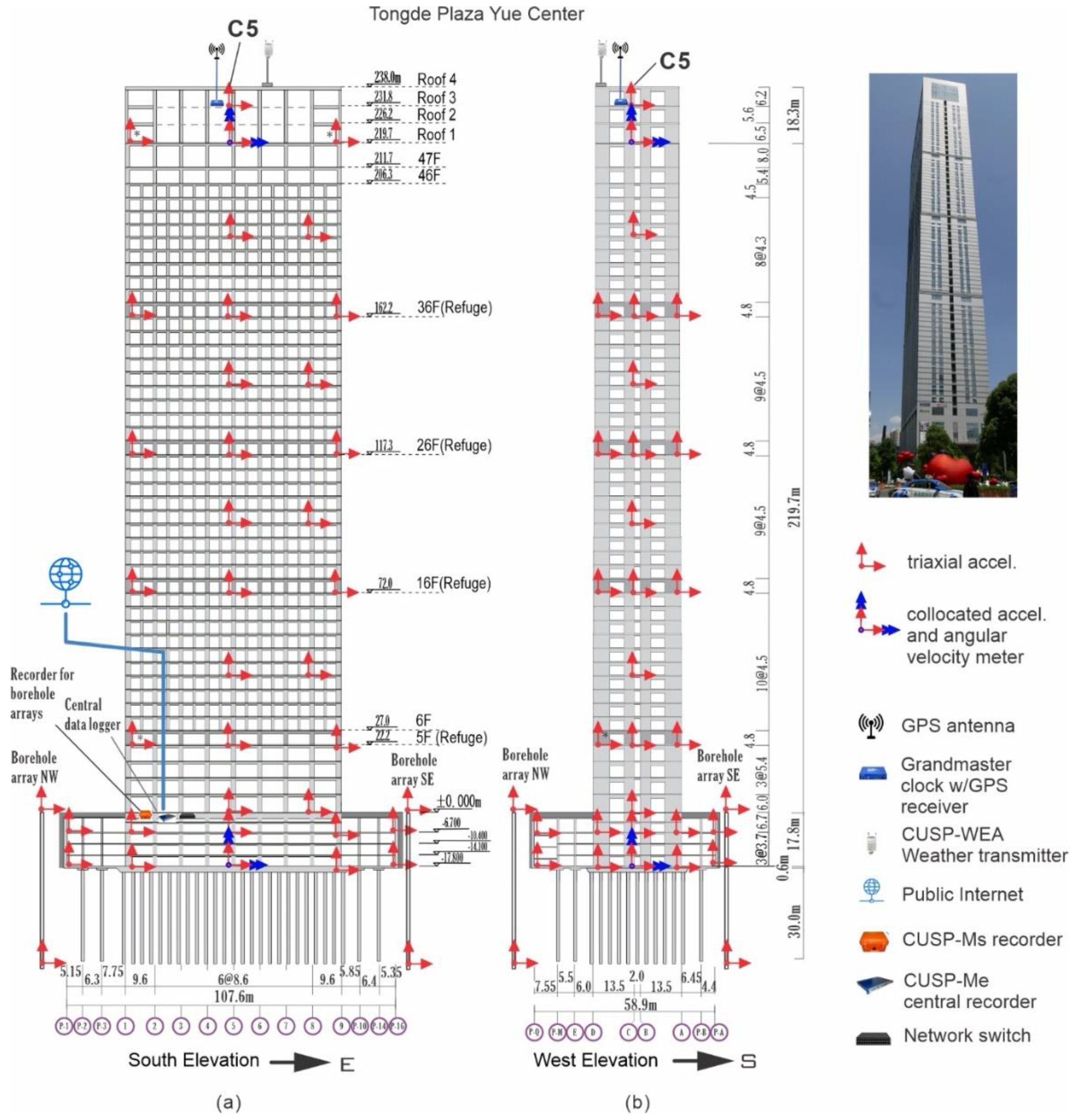
Figure 2.
Structural floor layout of TPYC. (a) Roof (F51), (b) floor 48F, (c) floors 5F to 45 F, (d) floors 1F to 5F, (e) floor -1B and (f) floor -4B.
Figure 2.
Structural floor layout of TPYC. (a) Roof (F51), (b) floor 48F, (c) floors 5F to 45 F, (d) floors 1F to 5F, (e) floor -1B and (f) floor -4B.
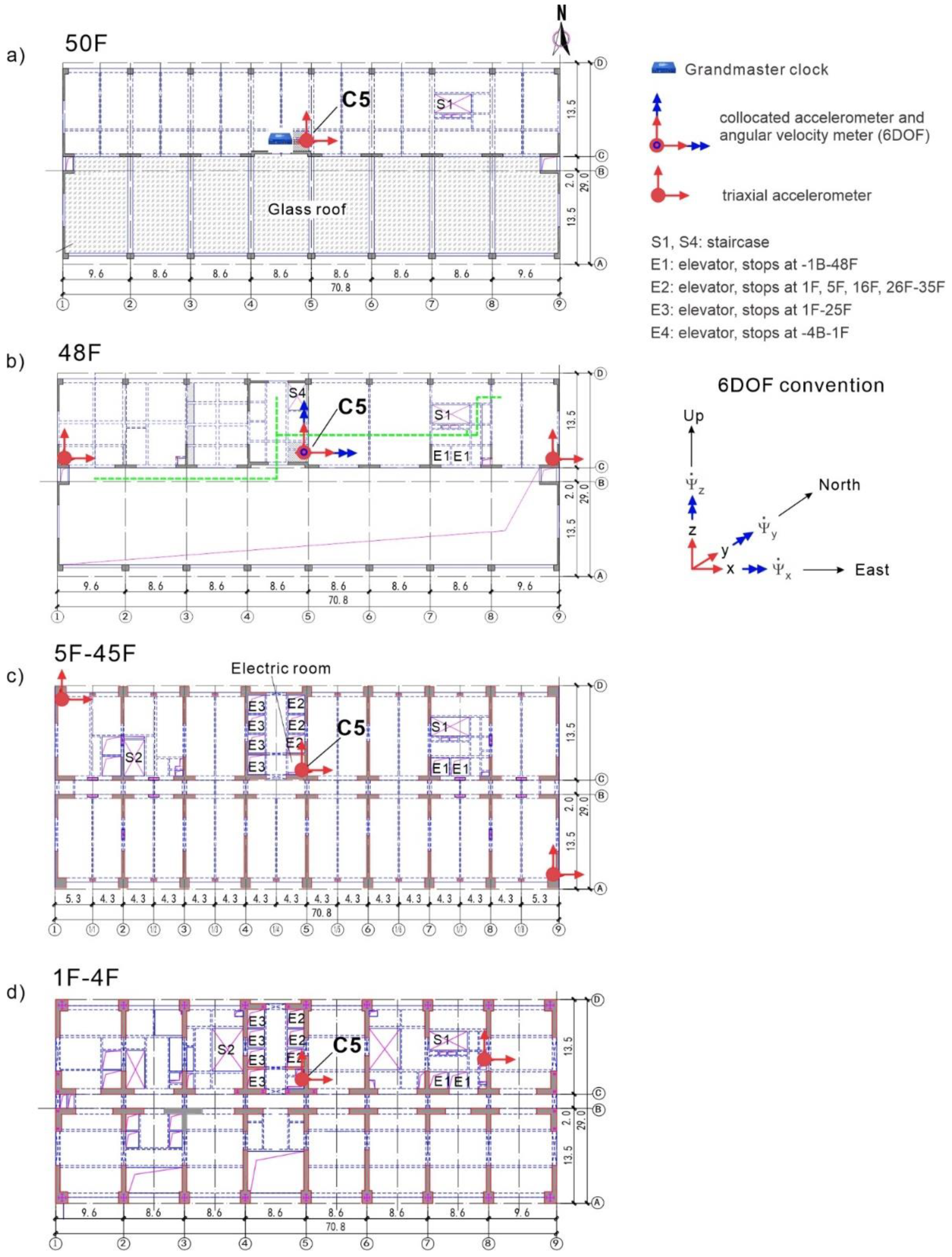
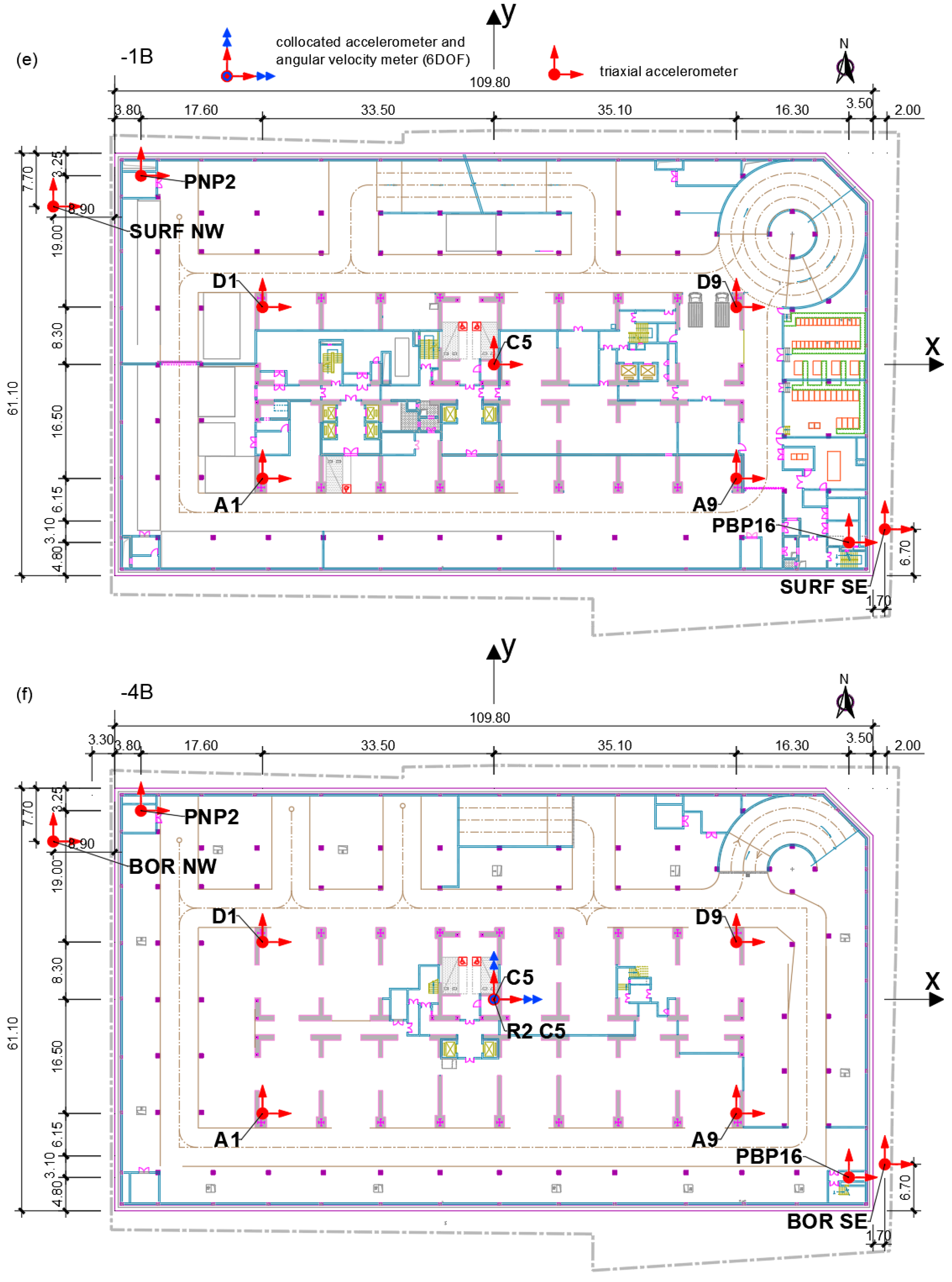
Figure 3.
shows the distribution of mass and lateral stiffness along the height in the Nort-South (NS) and East-West (EW) directions; the latter was obtained from a detailed finite element model of the tower, fixed at the ground floor [30].
Figure 3.
shows the distribution of mass and lateral stiffness along the height in the Nort-South (NS) and East-West (EW) directions; the latter was obtained from a detailed finite element model of the tower, fixed at the ground floor [30].
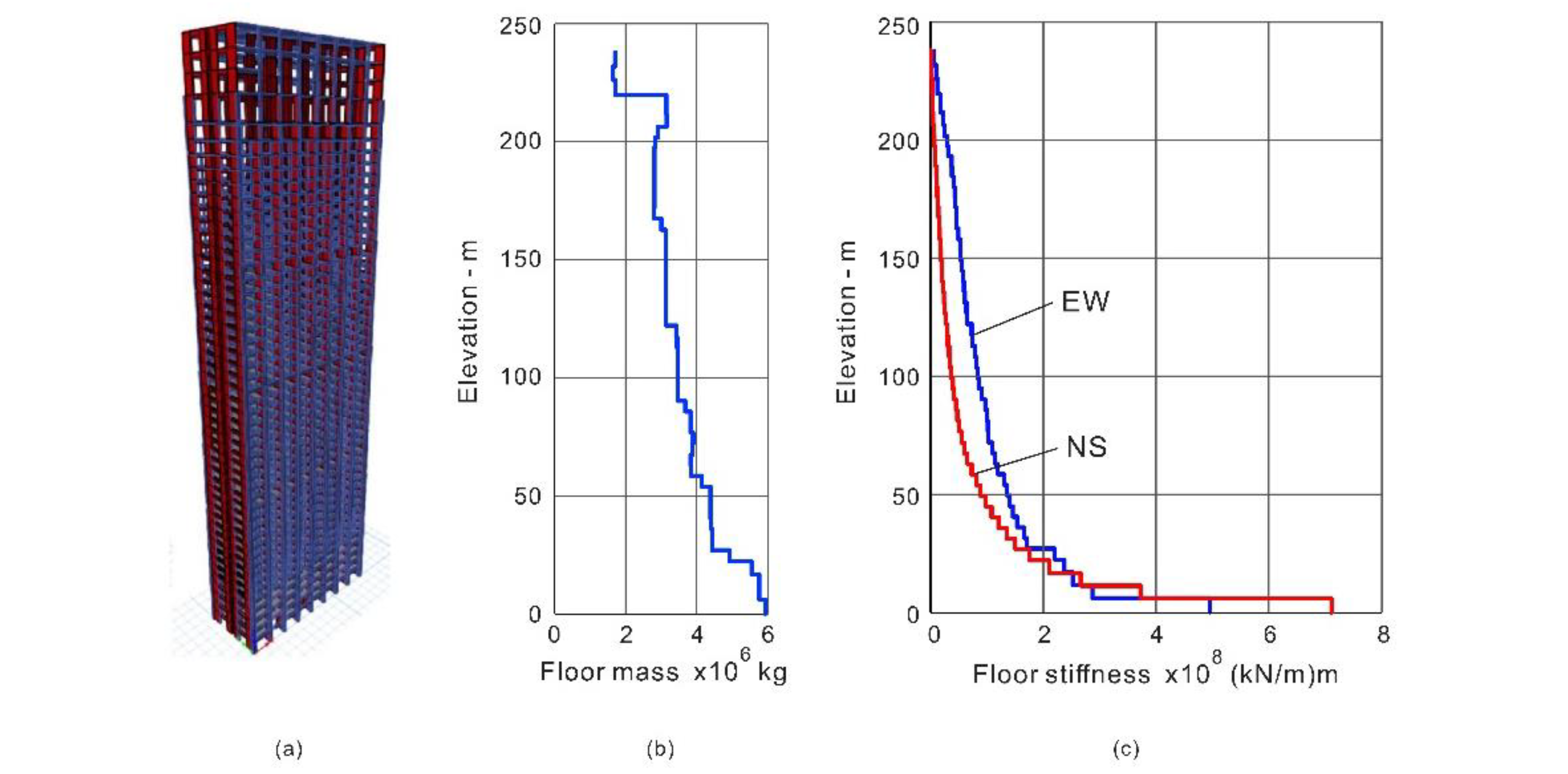
Figure 4.
Fitted model of the TPYC building, showing a detailed view of sensor locations, axis origins and directions, and fitted surfaces.
Figure 4.
Fitted model of the TPYC building, showing a detailed view of sensor locations, axis origins and directions, and fitted surfaces.
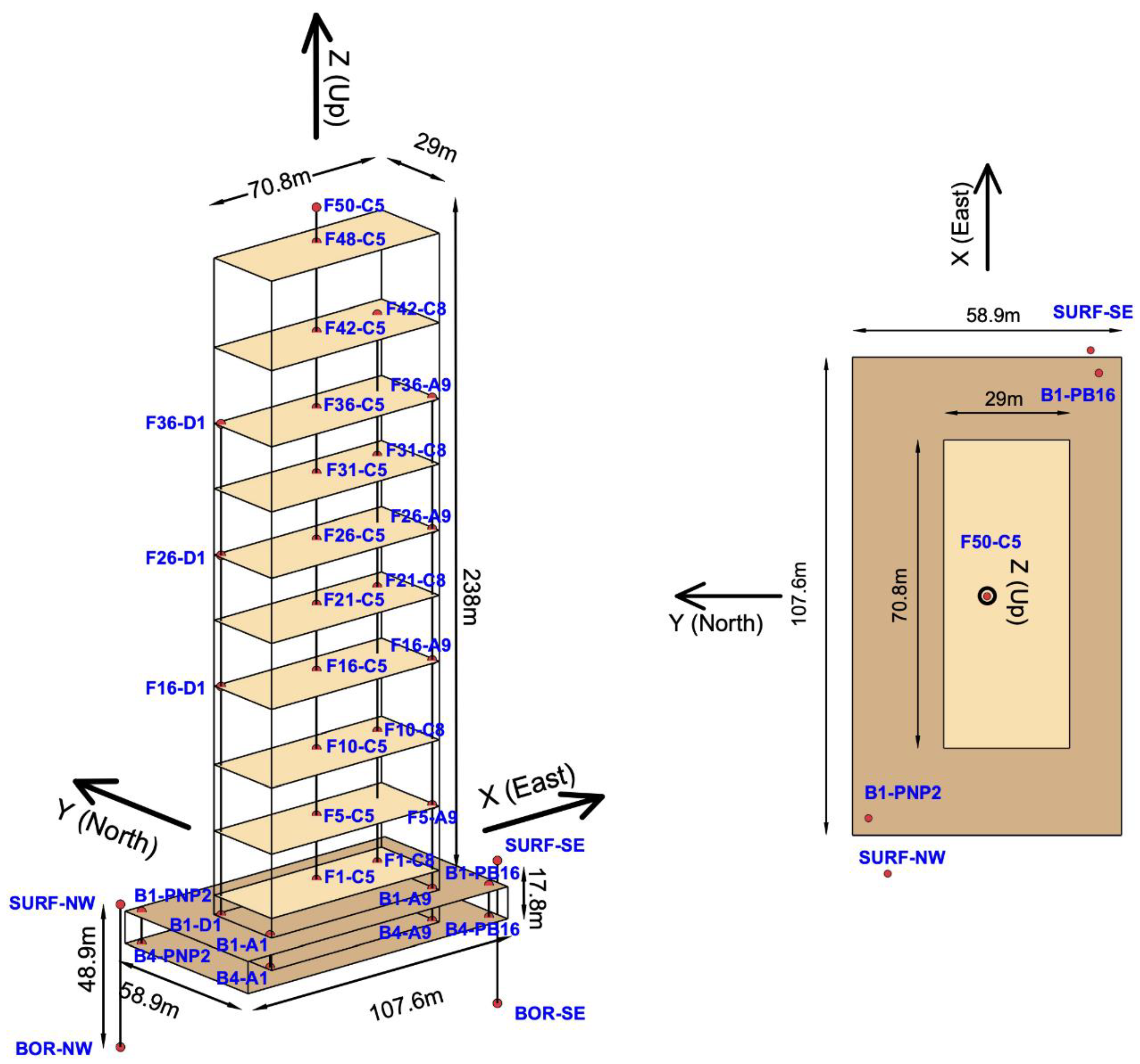
Figure 5.
Convention for the directions of the 6DOF motion.
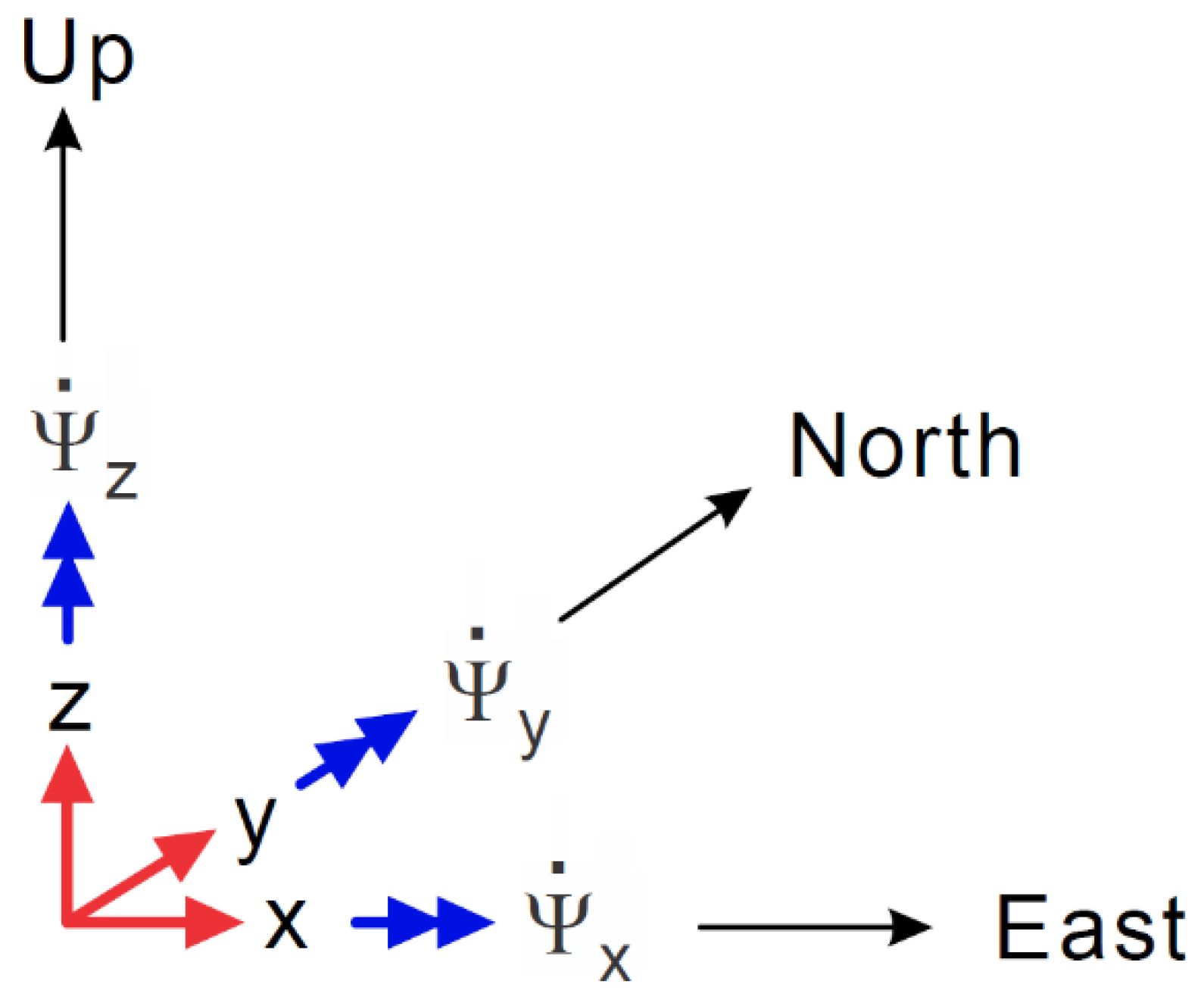
Figure 6.
Schematic representation of the slab of a floor instrumented with three sensors.
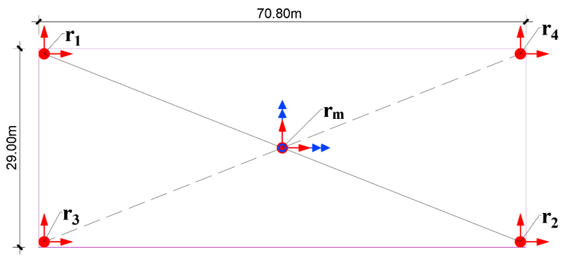
Figure 7.
Illustration of the steps in which different elements are added to the animation: a) slabs, b) structural boundaries, c) sensor locations and d) lines connecting neighboring sensors.
Figure 7.
Illustration of the steps in which different elements are added to the animation: a) slabs, b) structural boundaries, c) sensor locations and d) lines connecting neighboring sensors.
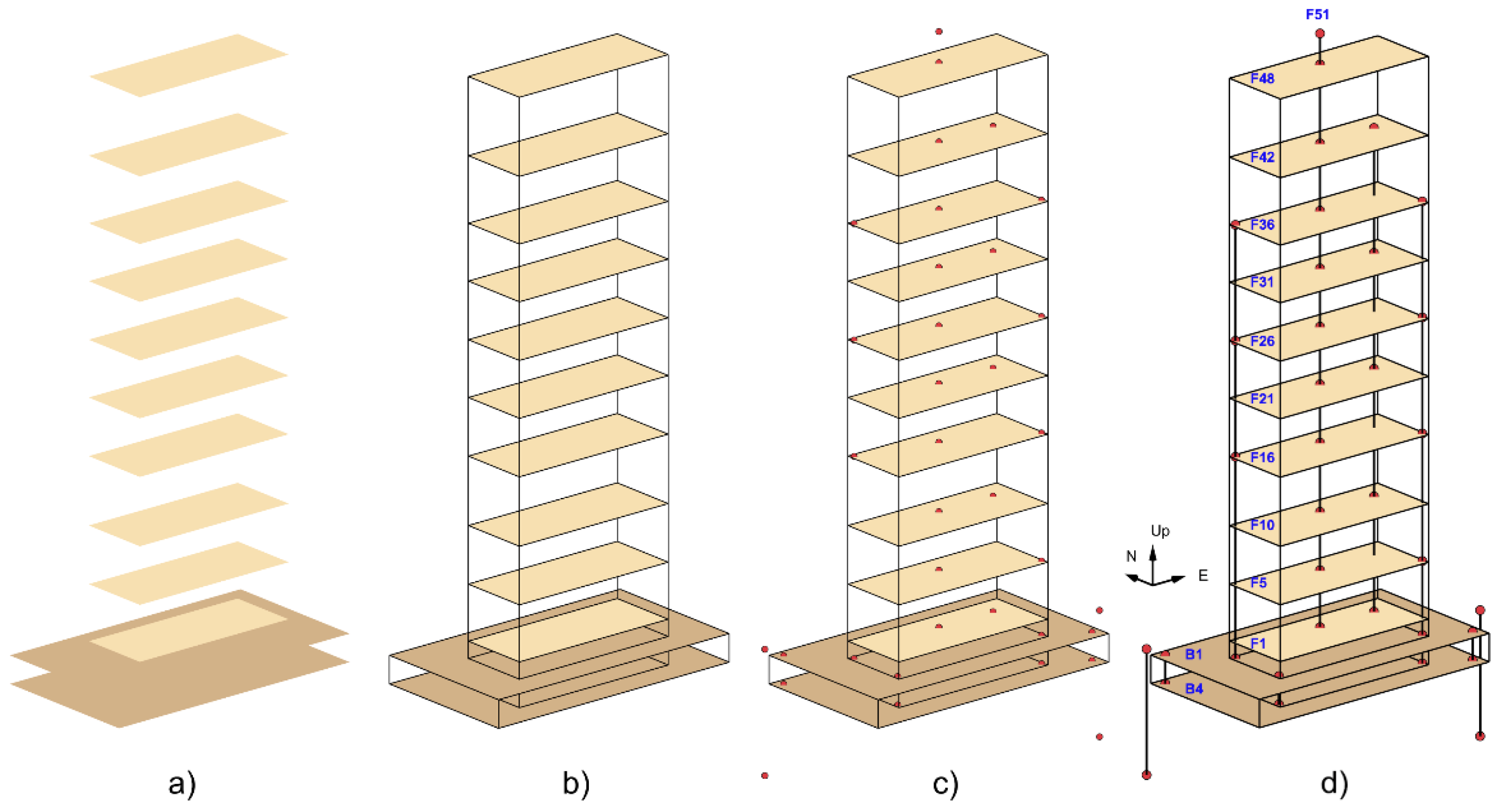
Figure 8.
Hodogram plots of the sensors located outside the building (SURF-NW, SURF-SE, BOR-NW, and BOR-SE); and are the radial and vertical components of the particle motion.
Figure 8.
Hodogram plots of the sensors located outside the building (SURF-NW, SURF-SE, BOR-NW, and BOR-SE); and are the radial and vertical components of the particle motion.
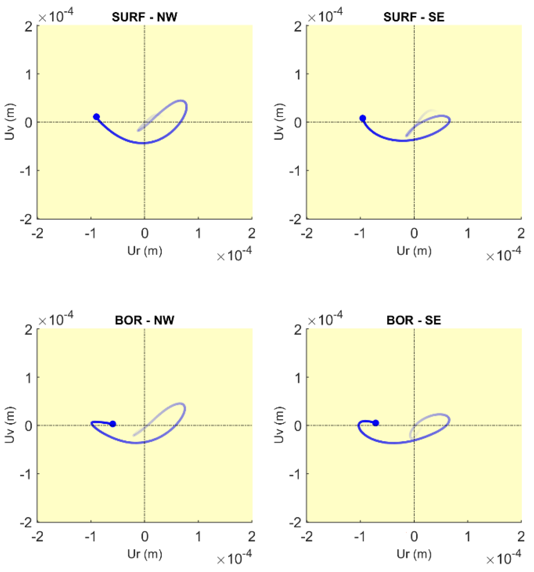
Figure 9.
Accelerations (the first 80 s) recorded during the Shuangbai earthquake of June 10, 2021, at different floors along column line C5 (floor centers). The motions recorded at the two borehole sensors are shown at the bottom. The motions were extracted from continuously recorded data.
Figure 9.
Accelerations (the first 80 s) recorded during the Shuangbai earthquake of June 10, 2021, at different floors along column line C5 (floor centers). The motions recorded at the two borehole sensors are shown at the bottom. The motions were extracted from continuously recorded data.
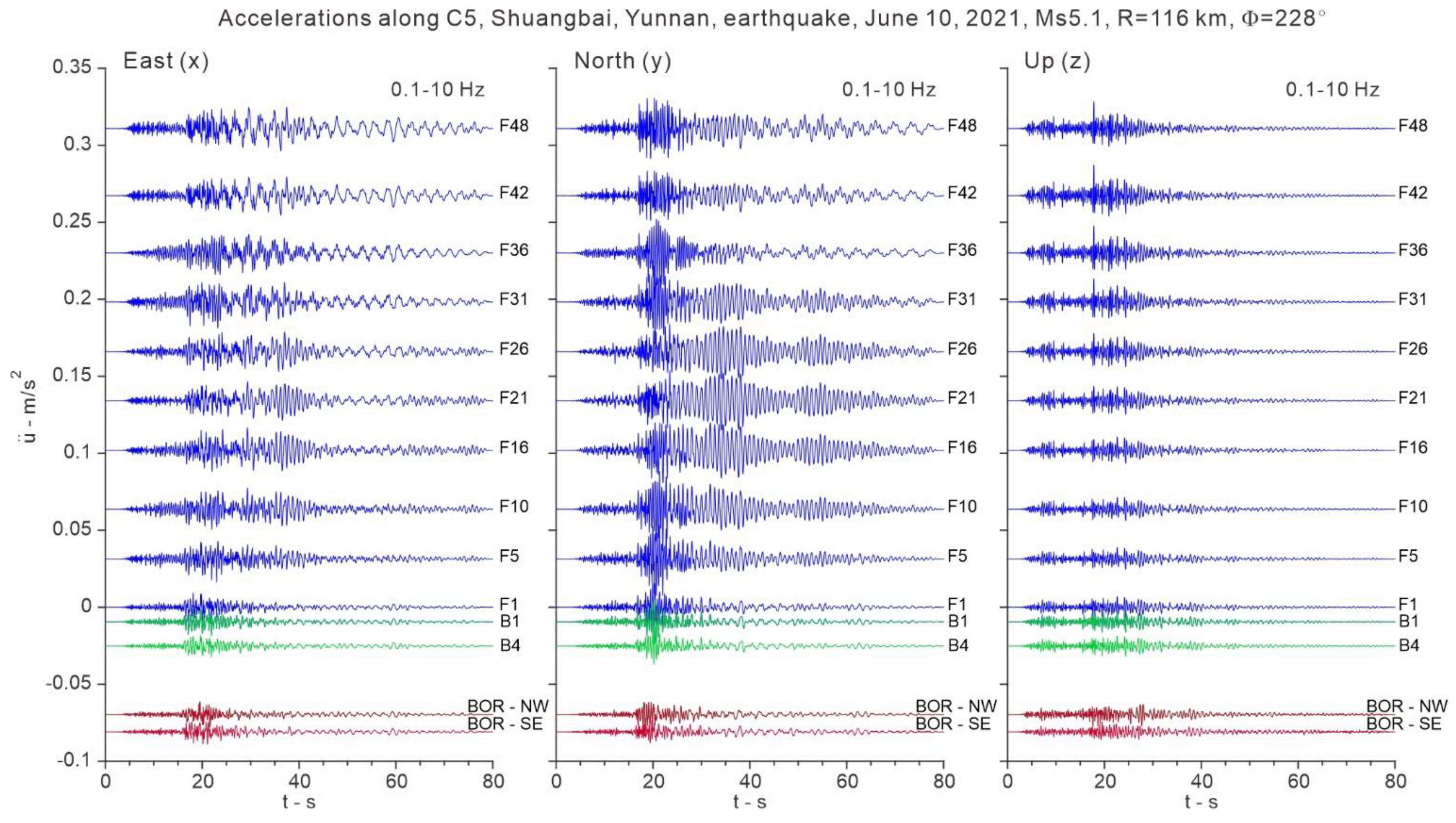
Figure 10.
Animation snapshot for the Shuangbai earthquake at time 22.84 s.
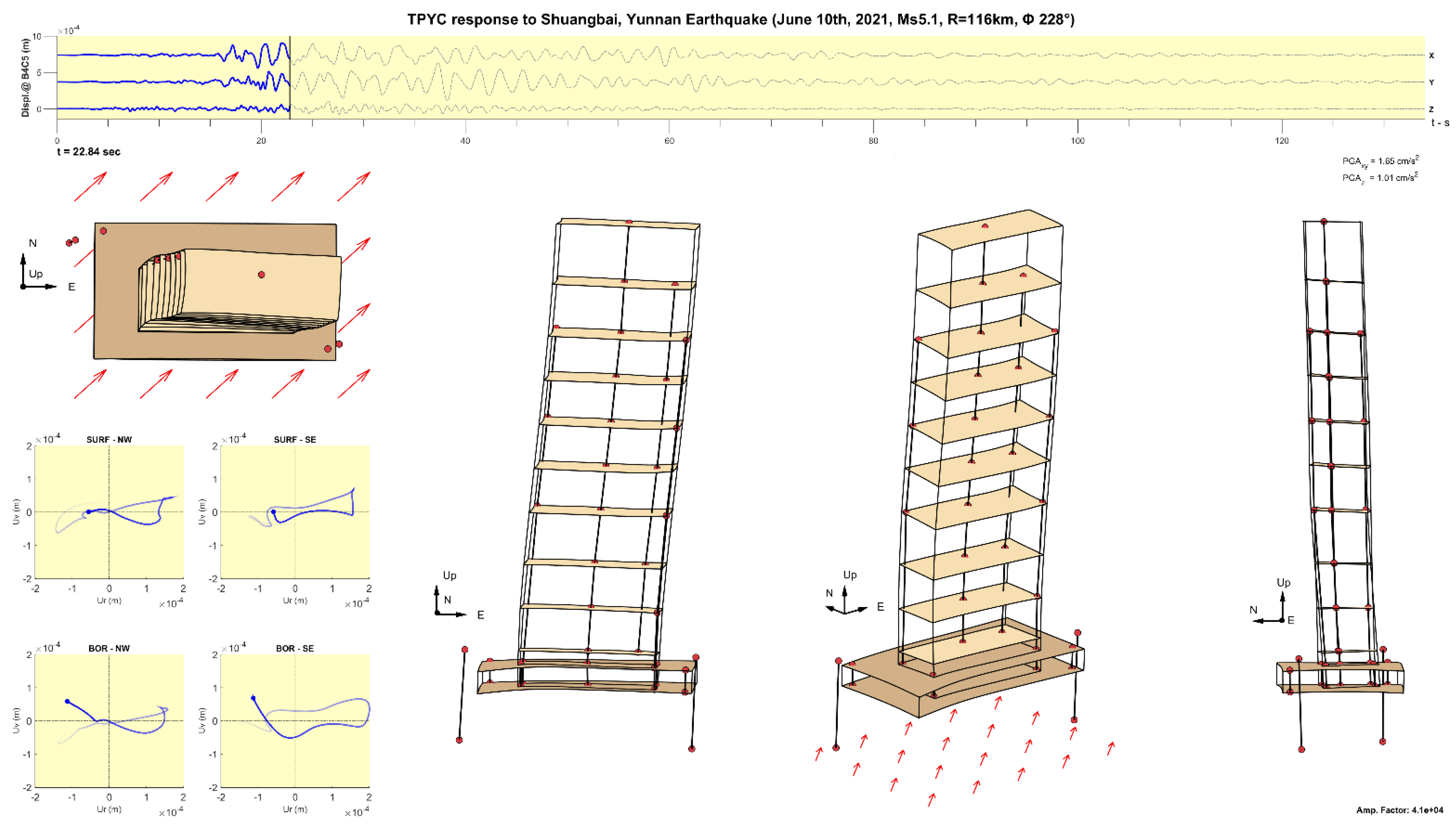
Figure 11.
Animation snapshot for the Shuangbai earthquake at time 23.95 s.
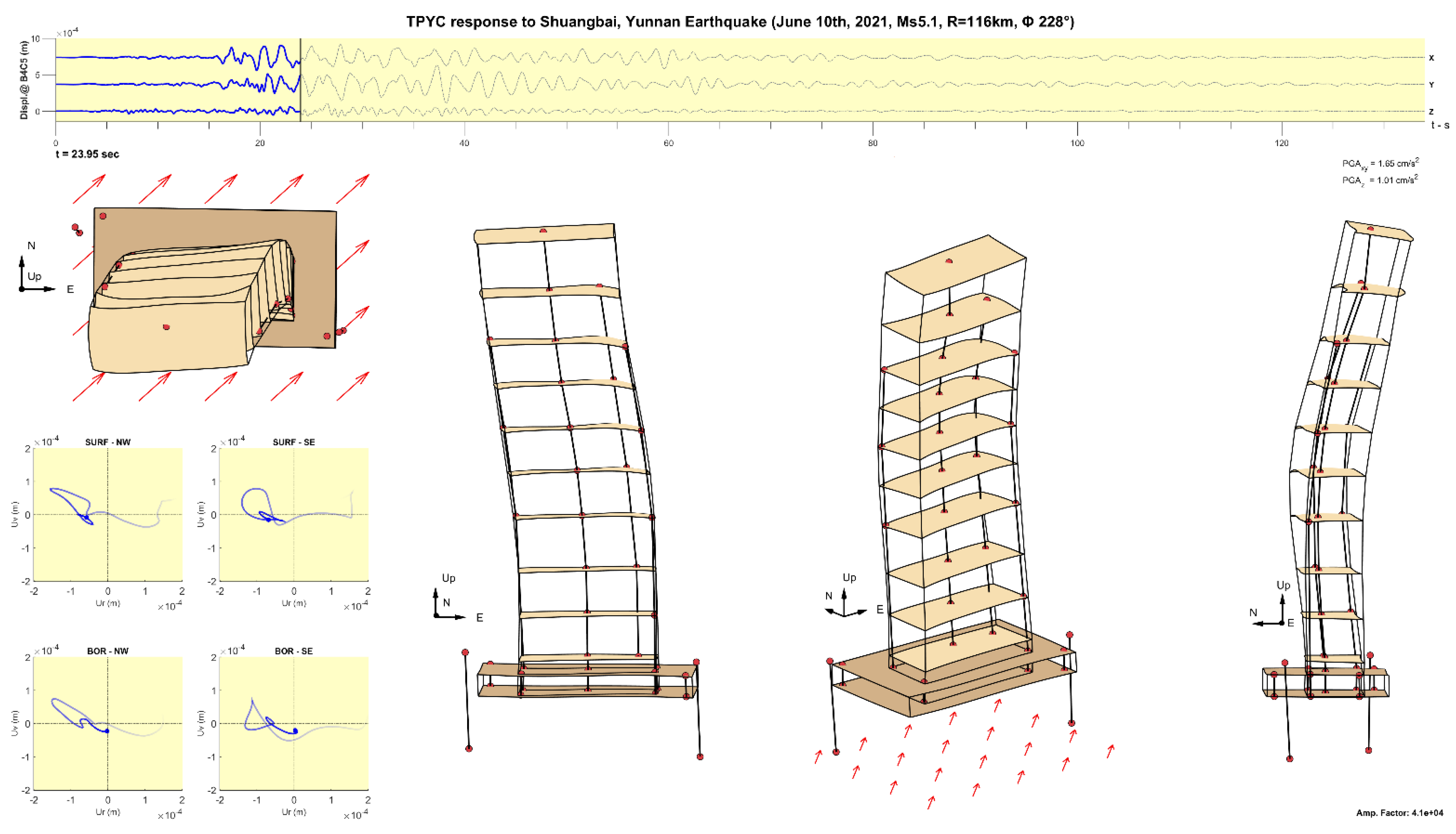
Figure 12.
Animation snapshot for the Shuangbai earthquake at time t = 29.62 s.
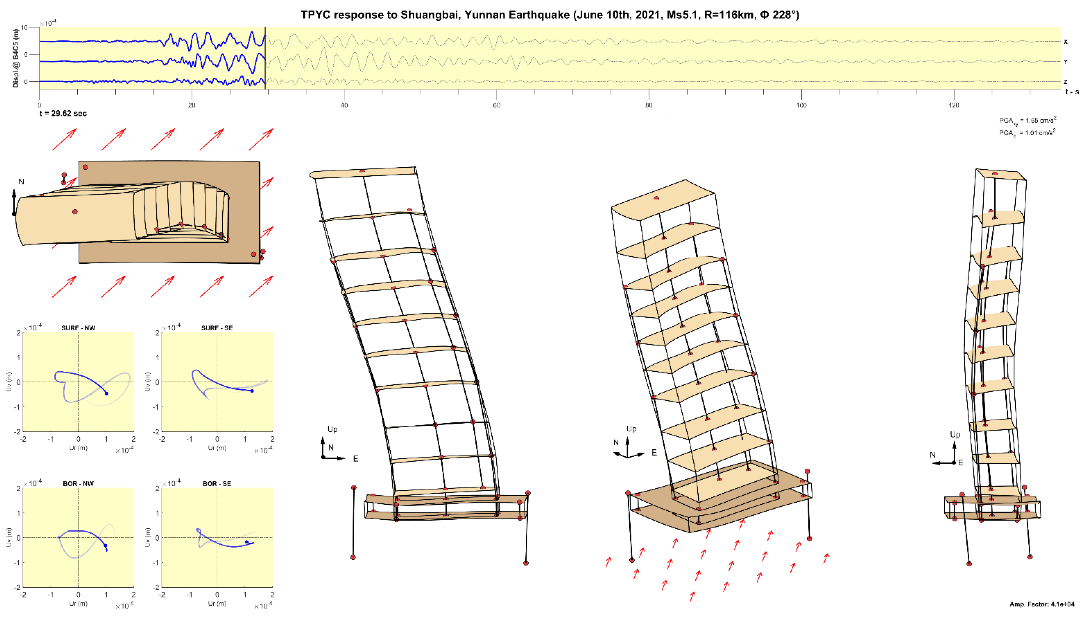
Figure 13.
Animation snapshot for the Shuangbai earthquake at time t = 31.00 s.
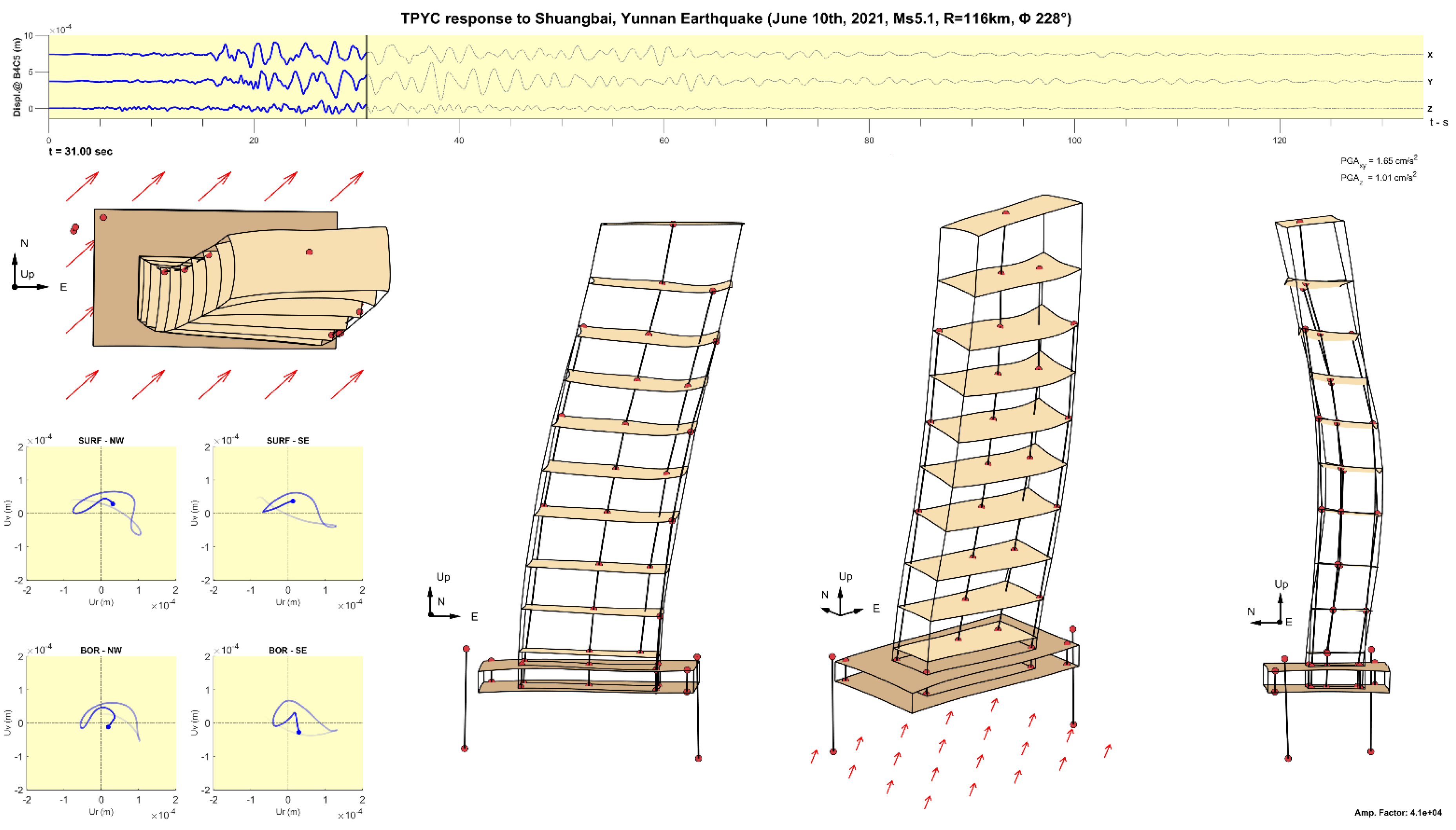
Figure 14.
Animation snapshot for the Shuangbai earthquake at time t = 32.20 s.
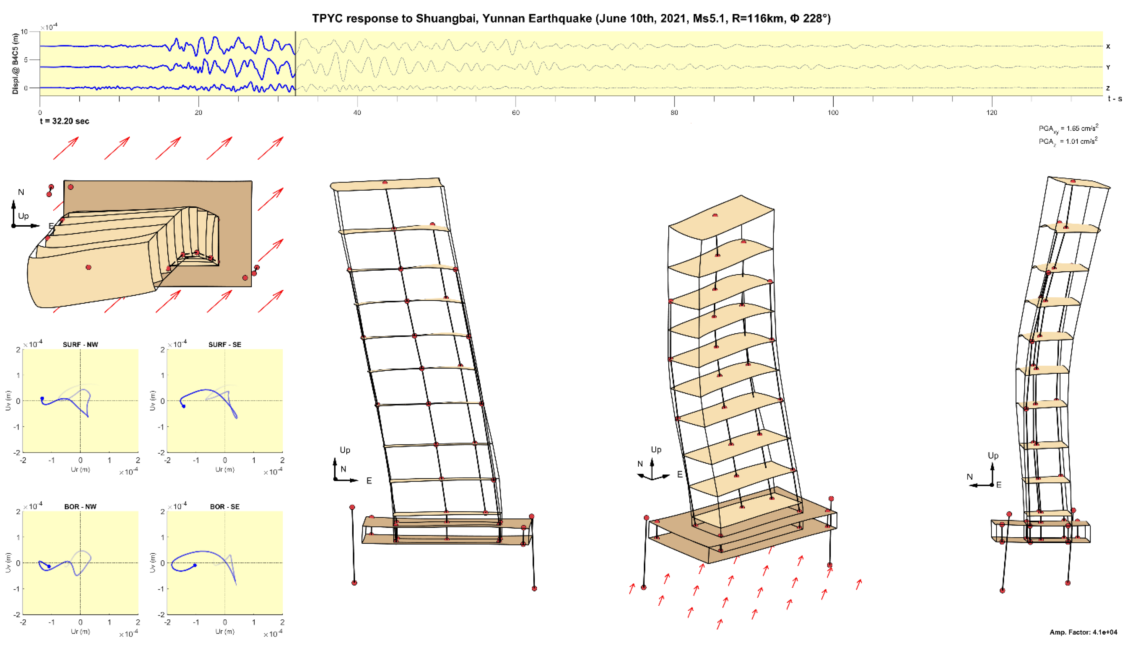
Figure 15.
Animation snapshot for the Shuangbai earthquake at time t = 40.93 s.
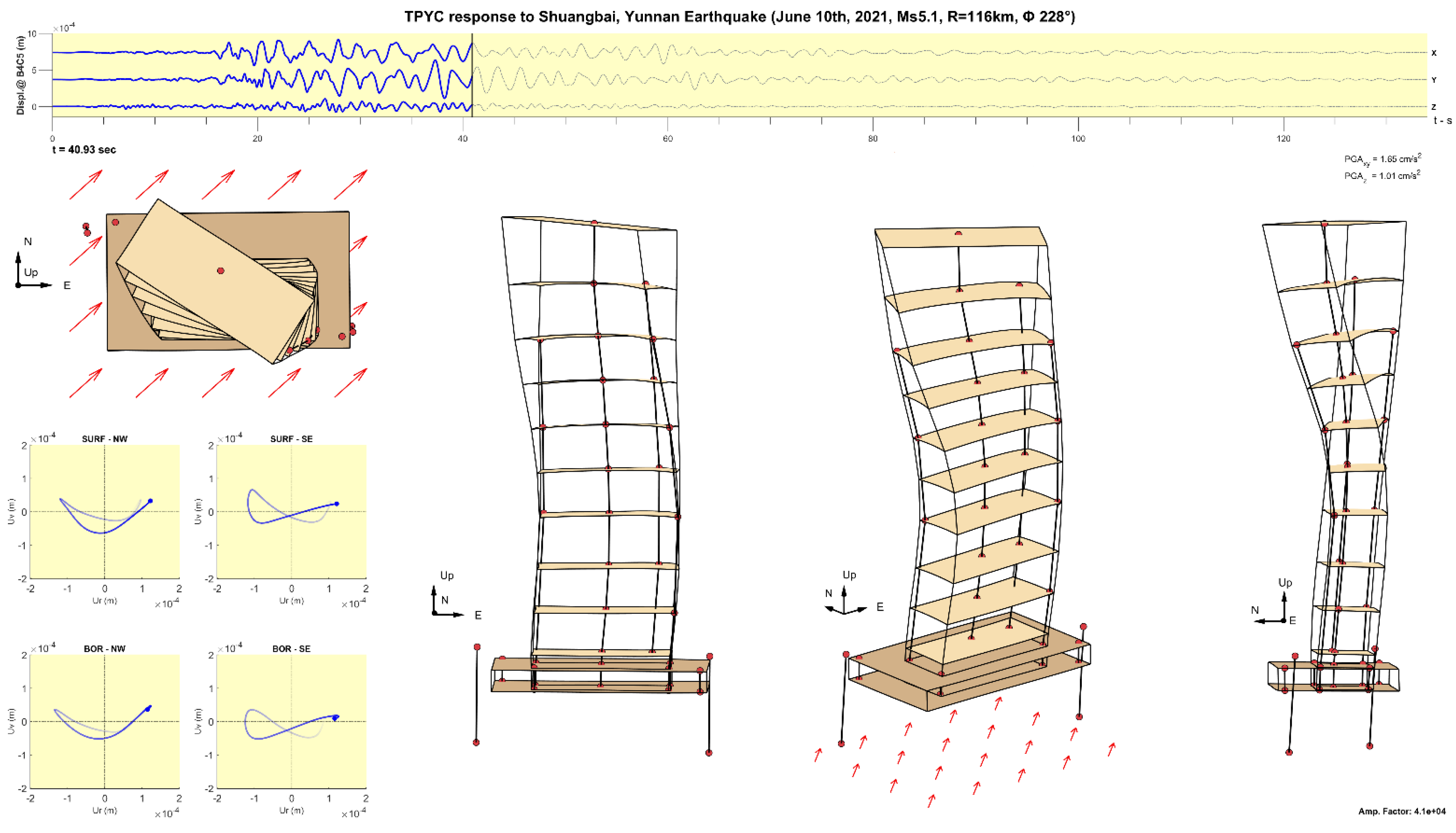
Figure 16.
Animation snapshot for the Shuangbai earthquake at time t = 43.93 s.
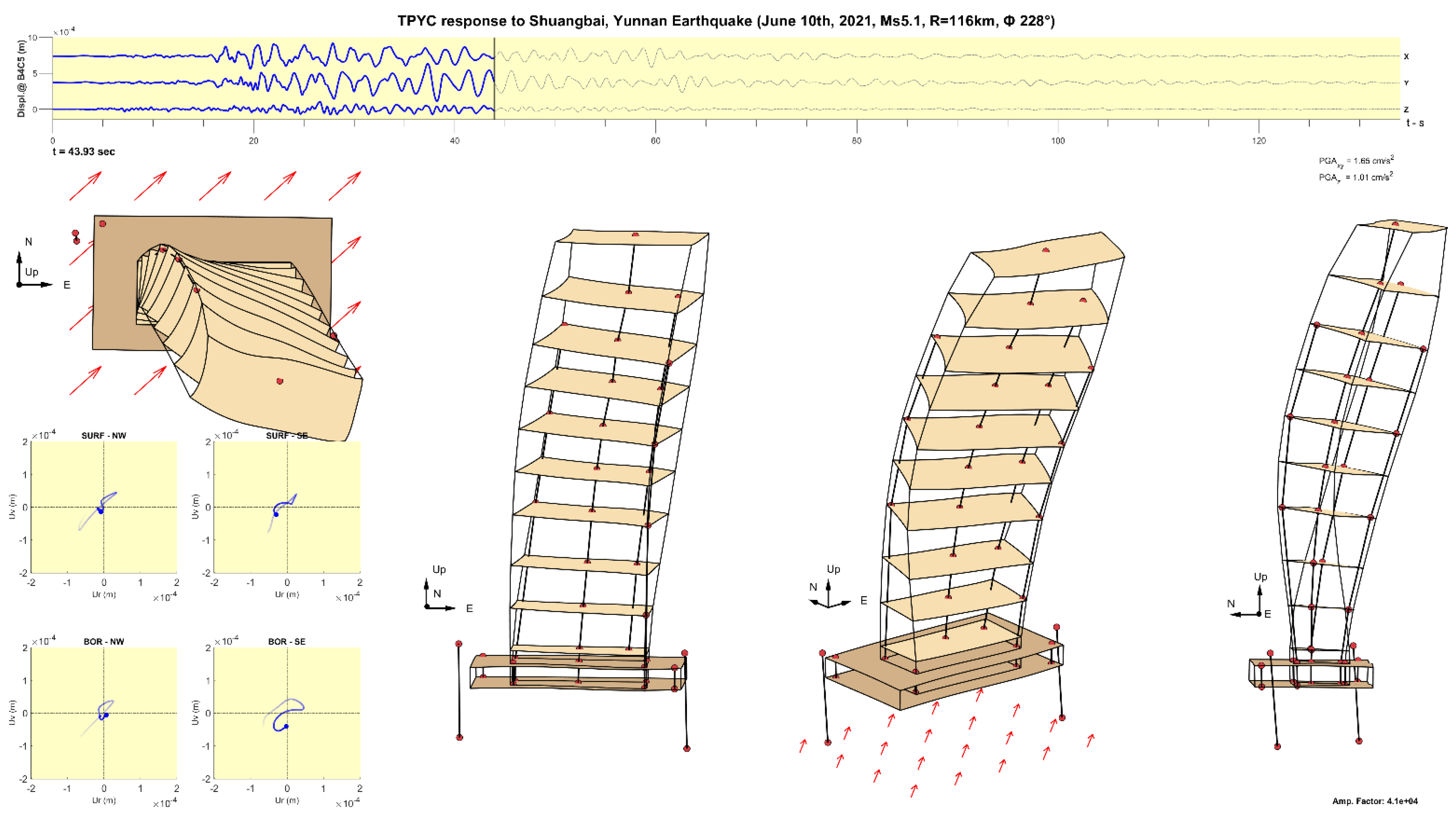
Figure 17.
Animation snapshot for the Shuangbai earthquake at time t = 50.44 s.
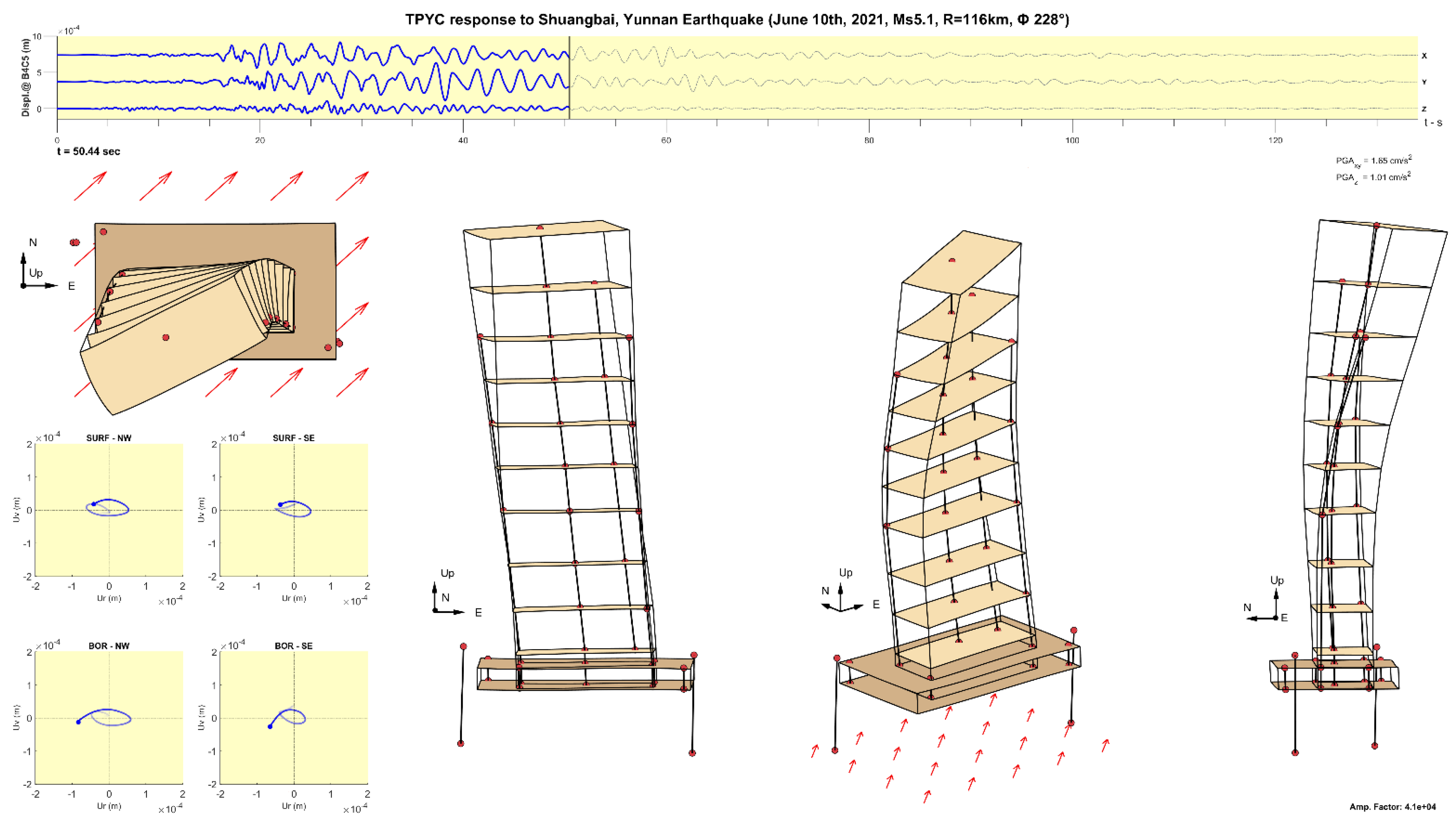

Table 1.
Points in the TPYC where motion is recorded.
| Sensors above ground level | Sensors below ground level | ||||||||
|---|---|---|---|---|---|---|---|---|---|
| Level | Point | X (m) | Y (m) | Z (m) | Level | Point | X (m) | Y (m) | Z (m) |
| F50 | F50 - C5 | 0 | 0 | 231.8 | B1 | B1 - PBP16 | 51.4 | -25.75 | -6.7 |
| F48 | F48 - C5 | 0 | 0 | 219.7 | B1 - PNP2 | -51.1 | 27.3 | -6.7 | |
| F42 | F42 - C8 | 25.8 | 0 | 188.9 | B1 - D9 | 35.1 | 8.3 | -6.7 | |
| F42 - C5 | 0 | 0 | 188.9 | B1 - A1 | -33.5 | -16.5 | -6.7 | ||
| F36 | F36 - A9 | 35.1 | -16.5 | 162.6 | B1 - A9 | 35.1 | -16.5 | -6.7 | |
| F36 - D1 | -33.5 | 8.3 | 162.6 | B1 - D1 | -33.5 | 8.3 | -6.7 | ||
| F36 - C5 | 0 | 0 | 162.6 | B1 - C5 | 0 | 0 | -6.7 | ||
| F31 | F31 - C8 | 25.8 | 0 | 140.1 | B4 | B4 - PBP16 | 51.4 | -25.75 | -17.8 |
| F31 - C5 | 0 | 0 | 140.1 | B4 - PNP2 | -51.1 | 27.3 | -17.8 | ||
| F26 | F26 - A9 | 35.1 | -16.5 | 117.3 | B4 - D9 | 35.1 | 8.3 | -17.8 | |
| F26 - D1 | -33.5 | 8.3 | 117.3 | B4 - A1 | -33.5 | -16.5 | -17.8 | ||
| F26 - C5 | 0 | 0 | 117.3 | B4 - A9 | 35.1 | -16.5 | -17.8 | ||
| F21 | F21 - C8 | 25.8 | 0 | 94.8 | B4 - D1 | -33.5 | 8.3 | -17.8 | |
| F21 - C5 | 0 | 0 | 94.8 | B4 - C5 | 0 | 0 | -17.8 | ||
| F16 | F16 - A9 | 35.1 | -16.5 | 72 | R2 | F48 - C5 - EQRR | 0 | 0 | 219.7 |
| F16 - D1 | -33.5 | 8.3 | 72 | B4 - C5 - EQRR | 0 | 0 | -17.8 | ||
| F16 - C5 | 0 | 0 | 72 | SURF | SURF - NW | -63.8 | 22.85 | 0 | |
| F10 | F10 - C8 | 25.8 | 0 | 45 | SURF - SE | 56.6 | -23.85 | 0 | |
| F10 - C5 | 0 | 0 | 45 | BOR | BOR - NW | -63.8 | 22.85 | -49.2 | |
| F5 | F5 - A9 | 35.1 | -16.5 | 22.2 | BOR - SE | 56.6 | -23.85 | -49.2 | |
| F5 - C5 | 0 | 0 | 22.2 | ||||||
| F1 | F1 - C8 | 25.8 | 0 | 0 | |||||
| F1 - C5 | 0 | 0 | 0 | ||||||
Disclaimer/Publisher’s Note: The statements, opinions and data contained in all publications are solely those of the individual author(s) and contributor(s) and not of MDPI and/or the editor(s). MDPI and/or the editor(s) disclaim responsibility for any injury to people or property resulting from any ideas, methods, instructions or products referred to in the content. |
© 2024 by the authors. Licensee MDPI, Basel, Switzerland. This article is an open access article distributed under the terms and conditions of the Creative Commons Attribution (CC BY) license (http://creativecommons.org/licenses/by/4.0/).
Copyright: This open access article is published under a Creative Commons CC BY 4.0 license, which permit the free download, distribution, and reuse, provided that the author and preprint are cited in any reuse.


