
Submitted:
10 November 2024
Posted:
12 November 2024
Read the latest preprint version here
Abstract
We describe the duality of incompressible Navier-Stokes fluid dynamics in three dimensions, leading to its reformulation in terms of a one-dimensional momentum loop equation. The momentum loop equation does not have finite-time blow-up solutions. The decaying turbulence is a solution of this equation equivalent to a string theory with discrete target space made of regular star polygons and Ising degrees of freedom on the sides. This string theory is solvable in the turbulent limit, equivalent to the quasiclassical approximation in a nontrivial calculable background. As a result, the spectrum of decay indexes is analytically computed, and it agrees very well with real and numerical experiments. Among the decay indexes there are complex conjugate pairs related to zeros of the Riemann zeta function. The Kolmogorov scaling laws are replaced by certain number theory functions, nonlinear in log-log scale.
Keywords:
Turbulence
; Fractal
; Fixed Point
; Velocity Circulation
; Loop Equations
1. Introduction
The incompressible Navier-Stokes (NS) equation is more than a partial differential equation with quadratic nonlinearity; it encapsulates deep hidden symmetries, reflecting the geometric nature of fluid flows. Arnold [1] first revealed the geometric aspects of fluid dynamics, showing the relationship between the evolution of fluid elements, preserving volume, and diffeomorphism groups.
This insight has sparked considerable mathematical investigation, yet it has not resolved the enduring problem of explosive solutions in NS dynamics. Power counting suggests that finite-time singularities (poles) might arise in the NS equation, but is a deeper mechanism preventing such outcomes?
In 1993, we introduced a new geometric approach to the NS equation called the loop equation [2]. This approach predicted the Area Law for the probability distribution of turbulent velocity circulation around large stationary loops, a prediction later confirmed numerically [3,4].
More recently, we found an exact solution to the loop equation [5], yielding explicit energy spectrum formulas for decaying turbulence, which closely align with experimental and simulation data [6].
This paper, however, focuses on the broader duality between fluid dynamics and a Schrödinger equation in loop space. This duality reveals a hidden one-dimensional quantum system underlying classical NS dynamics in any spatial dimension. The dimensional reduction and the quantum nature embedded in everyday fluids open new avenues for study.
We present a general framework for solving the NS equation’s Cauchy problem with rough initial data of finite variance . Classical solutions are recovered in the limit . From a physical standpoint, this limit is unnecessary, as real fluids always experience thermal noise, which the NS evolution can amplify or diminish over time.
We highlight five key features of this new representation:
- It uncovers a duality between classical fluid dynamics and quantum mechanics.
- It reduces the problem from to dimensions, introducing fractal curves as solutions.
- It allows for exact solutions characterized by fixed trajectories.
- The explosive solutions are ruled out.
2. Loop Functional and its General Properties
The loop functional is defined as a phase factor associated with velocity circulation, averaged over the initial distribution of the velocity field
We use viscosity as a unit of circulation. Both have the same dimension as the Planck’s constant ℏ. The viscosity will play the same role in our theory as Planck’s constant in quantum mechanics. The variable with this definition is dimensionless.
This loop functional is the Fourier transform of the PDF for the circulation over fixed loop C
There is an implicit dependence of time, coming from the evolution of the velocity field by the Navier-Stokes equation
We restrict ourselves to three-dimensional Euclidean space, the most interesting case for physics applications. The generalization to arbitrary dimension is straightforward, as discussed in previous papers [2,5,7].
In the next sections, we shall study the Cauchy problem for the loop equation [2,7], which follows from the Navier-Stokes equation. Here, we state some general properties of the loop function and various scenarios of its evolution.
The first obvious property is that this evolution goes inside the unit circle
At a small enough time passed from initial data, , turning off the noise would bring us to the usual unique laminar solution of the Navier-Stokes equation, corresponding to the loop functional at the unit circle with a small enough phase.
Here, denotes the variance of the Gaussian distribution of the velocity field around some smooth initial value. Generally speaking, we could expect the following fixed points (see Fig.Figure 1) of the time evolution for the loop functional1.
- Finite-time explosion? The vorticity could blow up at some finite or infinite point in time, leading to infinite circulation. In this case, the loop functional would cover the unit circle at this moment of singularity.
In the following sections, we elaborate on each of these possible regimes. The finite-time explosion is proven to be inconsistent and is therefore ruled out.
3. Loop Equation
The first step is to write down the loop equation by projecting the Hopf equation to the loop space.
Before doing that, we have to specify certain boundary conditions which we assume in our fluid dynamics. Namely, we consider infinite space, with boundary condition of vanishing or constant velocity at infinity.
Vorticity can be everywhere in space, but not at infinity, where the velocity gradients vanish by our boundary conditions. We also assume that there are no internal boundaries, such as the surfaces of the bodies which our fluid flows around. We do not eliminate some surfaces with singular vorticity in the limit of zero viscosity, such as vortex lines and sheets, as long as these singular regions are located in a finite part of the volume, in agreement with our boundary conditions. At finite viscosity, these regions have finite thickness proportional to , which leads to anomalous dissipation in the turbulent flow.
The computations leading to the loop equation were performed in the old papers [2,7]. For the reader’s convenience, we repeat them here using another language, hopefully more clear for mathematicians.
The straightforward time derivative of the loop functional, assuming the constant loop C and using time derivative (5) of the velocity field in the circulation, yields
The averaging goes, as before, over all NS solutions with a given set of initial values . It is implied that a probability measure (see examples below) is supplied for this set of initial velocity fields. The phase factor of circulation is averaged over initial data using this measure.
The gradient terms in (5) dropped in the time derivative of the circulation as the integral of a gradient of some single-valued function of coordinate around the closed loop:
The velocity field is a solution of the Poisson equation, relating it to vorticity by incompressibility condition
This representation leaves vorticity as the main unknown variable in the time derivative of the loop functional.
To find the loop equation, we must replace the vorticity and its gradients with certain operators acting on the loop independently of the vorticity and velocity fields. As a result of such transformation, the vector function will be replaced by a certain operator in loop space acting on
As this operator does not depend on the dynamical variables , it can taken out of the averaging over trajectories starting from various initial data , so that this operator acts on the loop average . Such is the plan of the proof of the loop equation. We define the loop operators and follow this plan in the next section.
4. The Definitions Of The Loop Operators And The Proof Of The Loop Equation
The operators in the loop equation were introduced in[2] and explained at length in my review paper [7].
In this paper, we do not assume any knowledge of the previous work; instead, we derive the loop operators from scratch using a simpler method.
First, we replace the smooth loop C by a polygon with N sides with the vanishing length in the limit . We postpone this local limit until we solve the discrete loop equation. This limit will define the continuum theory in the same way as in the QFT; the functional integral is discretized using a lattice with the lattice spacing going to zero at the end of the calculation. In this limit, the theory’s parameters vary with the lattice spacing to provide a finite result for the physical observables.
The first observation is that with smooth velocity and finite vorticity field, the discrete circulation around the polygon converges to the circulation around the smooth loop
The finite difference becomes derivative for the smooth loop; the error will vanish as .
The next property is also easy to prove using the Stokes theorem for a small triangle
This first derivative vanishes as in the local limit.
The second derivative, however, stays finite. We prefer to use another set of variables
The last relation follows from the chain rule
The vorticity can be represented as
Finally, the velocity field at the vertex can be related to the vorticity through the Biot-Savart law
Let us verify this relation using the Biot-Savart integral formula for the inverse Laplace operator
At first glance, the loop in the new circulation involves two long "wires": and .
However, in the local limit, when the distance , these two wires have zero area inside the arising thin triangle, so they effectively cancel in virtue of the Stokes theorem, assuming the Biot-Savart integral converges.
This produces the desired result in the Biot-Savart formula.
The convergence of the Biot-Savart integral follows from our boundary conditions, assuming no vorticity at infinity or even stronger requirement of finite support of vorticity. The phase factor does not influence the absolute convergence, so it can be set to for that purpose and taken out of the integral, returning us to the convergence of the ordinary Biot-Savart integral.
Therefore, with accuracy, we can replace the right side of the (10) by its discrete version with operators involving
We restrict ourselves to the velocity vanishing at infinity and no internal boundaries in the physical domain. With this boundary condition, the harmonic potential is zero, and there is no zero mode to add to the inverse Laplace operator.
In the rest of the paper, we shall use the language of the continuum theory, implying the limit of a polygon with N sides. While the lengths of the sides of vanish in the local limit , the sides of polygon are not at our disposal, so they may stay finite (this will happen in the decaying turbulence below).
5. SchröDinger Equation In Loop Space
Before we investigate the solutions of the loop equation, let us consider its physical and mathematical meaning and its relation to the geometry of the incompressible flow.
By definition, the loop functional is a superposition of the phase factors with the circulation of a particular solution of the Navier-Stokes equation. These solutions have initial values , distributed by some distribution which we assume Gaussian with the mean given by some smooth initial field and some coordinate-independent variance .
In the turbulent scenario, the Navier-Stokes trajectories initiated from a narrow vicinity of some smooth velocity field eventually expand and cover some attractor, slowly varying with time and asymptotically converging to .
The alternative smooth solution of the Navier-Stokes equation, sought after in numerous mathematical papers, would correspond to these trajectories staying close and converging to a single trajectory in the limit . This single trajectory would go along the unit circle, bounding our disk.
With this generalization of a definition of the Cauchy problem for the Navier-Stokes equation, we can address the existence of smooth, explosive, or stochastic (i.e., turbulent) solutions within the loop equation’s framework.
The transformation from the Navier-Stokes equation to the loop equation is similar to that from the Newton equation of the particle in random media to the diffusion equation. We add dimension to the problem, switching to the probability distribution in , after which the particle’s infinitesimal time steps translate into probability derivatives by coordinates.
There are two essential differences, however. Our loop space is not just higher-dimensional; it is infinite-dimensional. The second difference is that in addition to diffusion in loop space, we have nonlocal terms affecting the evolution of the distribution in loop space.
Our definition of the loop functional already by construction has superficial similarities with quantum mechanics. We are summing phase factor over a manifold of solutions of the Navier-Stokes equations. The circulation plays the role of classical Action, and viscosity plays the role of Planck’s constant.
This analogy becomes a complete equivalence when the time derivative of the loop functional is represented as an operator in the loop space acting on this functional.
Now we have quantum mechanics in loop space, with the Hamiltonian
The operator depends of functional derivatives , as was determined, and discussed in previous works [2,5,7]. Our polygonal approximation has no functional derivatives, just ordinary derivatives . Thus, our quantum-mechanical system has continuum degrees of freedom.
This Hamiltonian is not Hermitian, which reflects the dissipation phenomena. The time reversal leads to complex conjugation of the loop functional, a nontrivial transformation, as there is no symmetry for the reflection of velocity field .
The loop in our theory is a continuous (but not necessarily differentiable) periodic function of the angular variable . Geometrically, this is a map of the unit circle into Euclidean space . In particular, there could be several smaller periods, in which case this loop becomes a set of several closed loops connected by backtracking wires like in Fig.Figure 2.
Also, this map could have an arbitrary winding number n corresponding to the same geometric loop in traversed n times.
The linearity of the loop equation is the most important property of this transformation from Navier-Stokes equation to the quantum mechanics in loop space.
This transformation is an example of how the nonlinear PDE reduces to the linear problem projected from high dimensional space. In our case, this space is the loop space, which is infinite-dimensional.
As a consequence of linearity, the generic solution of the loop equation is a superposition of particular solutions with various parameters. More generally, this is an integral (or sum, in discrete case) over the space of solutions of the loop equation.
In the case of the Cauchy problem in loop space, the measure for this integration over space is determined by the initial distribution of the velocity field. The asymptotic turbulent solution [5] uniformly covers the Euler ensemble, like the microcanonical distribution in Newton’s mechanics covers the energy surface.
This turbulent solution does not solve a Cauchy problem; it rather solves the loop equation with the boundary condition at infinite time .
In the next section, we simplify the loop equation using Fourier space; this will be the foundation for the subsequent analysis.
6. Momentum Loop Equation
The loop operator, in (28), dramatically simplifies in the functional Fourier space, which we call momentum loop space. In our discrete approximation the momentum loop will also be a polygon with N sides.
The origin of this simplification is the lack of direct dependence of the loop operator on the loop C itself. Only derivatives enter this operator.
From the point of view of quantum mechanics in loop space, our Hamiltonian only depends on the canonical momenta but not on the canonical coordinates. This property is exact as long as we do not add external forces.
This remarkable symmetry property (translational invariance in loop space) allows us to look for the "plain wave" Ansats:
The discrete loop equation (28) would be satisfied provided satisfies the following momentum loop equation (MLE)[5,7]
In the local limit , the momentum loop will have a discontinuity at every parameter , making it a fractal curve in complex space . Such a curve can only be defined using a limit like a polygonal approximation.
You can regard this curve as a periodic random process hopping around the circle (more about this process below, in the context of the decaying turbulence).
Generally, there is also a discontinuity at the endpoint, making this momentum loop open . With open momentum loop, the loop functional is not translational invariant
7. Uniform Constant Rotation And Momentum Loop
The loop equation has several unusual features, especially the discontinuities of the momentum loop. These discontinuities have a physical meaning related to vorticity.
It is best understood by studying an exact fixed point of the loop equation: the global constant rotation. We set for simplicity in this example.
We present two implementations of the momentum loop for this simple model: one using an infinite Fourier expansion and another using the limit of polygonal approximation of the loop. This will allow us better understand the origin and the meaning of these discontinuities.
7.1. Infinite Fourier Series
Here is the implementation of the momentum loop by an infinite Fourier series.
The covariance matrix components are (for odd )
The loop functional is obtained after averaging over Gaussian random variables . The loop function can be computed without an explicit Functional Fourier transform using the well-known properties of the Gaussian expectation value of the exponential.
With this representation, it is obvious why the circulation does not depend on time; the vorticity is a global constant which does not depend on time nor . Simple tensor algebra in the time derivative of circulation leads to the term
The tensor trace vanishes by symmetry , changing the sign of . This solution is a consequence of the rotational symmetry of the Navier-Stokes equation.
Verification of the MLE is more tedious because, this time, the velocity in (38) explicitly depends on the coordinate. This will become in the equation, which means that the operator depends both on . Still, for the proof, it suffices to know the momentum loop (Section 6) and the corresponding velocity field (38), solving the Navier-Stokes equation for arbitrary constant .
Though this special solution does not describe isotropic turbulence, it helps understand the mathematical properties of the loop technology.
In particular, it shows the significance of the discontinuities of the momentum loop , as it is manifest in the correlation function(46). These discontinuities are necessary for vorticity; they result from the divergence of the Fourier series in (42).
The mean vorticity at the circle is proportional to independently of
7.2. Polygonal Approximation
The second implementation is more aligned with the methods we use in the MLE. We approximate the loop C as a polygon with vertices equidistant on a parametric circle.
Our next task is to represent the loop functional as a Gaussian average over the momentum loop } with symmetric covariance matrix
This representation will involve the following discrete Fourier transform with Gaussian coefficients
This discrete Fourier transform for reads
Note that this is antiperiodic: it changes the sign when the index goes around the loop. This, however, keeps the solution simply periodic in C space, as only even number of variables have non-vanishing expectation values in this particular example.
This example shows both the discontinuities’ meaning and the momentum loop’s approximation by a polygon. In this example, the continuum limit can be taken for the loop functional, but not at the level of the Fourier series for the momentum loop.
The formal limit exists for at fixed n
and matches the continuum theory, but the oscillating sum of Gaussian random variables does not converge to any normal function; rather, this is a stochastic process on with convergent expectation values.
8. Cauchy Problem And Its Solution
The Cauchy problem, notoriously difficult for nonlinear PDE, can be solved analytically for the loop equation. The hard part of the problem is now hidden in the limit , bringing us back to the Navier-Stokes equation with smooth initial data.
Let us describe this solution. Assuming the MLE (35) satisfied, we have certain conditions for the initial data . This data is distributed with some distribution to be determined from the equation
This path integral is nothing but a functional Fourier transform, which can be inverted as follows
The definition of the parametric-invariant functional measure in this Fourier integral was discussed in detail in the old work [2,7]. The periodic vector functions are represented by the Fourier series, after which the measure becomes a limit of the multiple integrals over all the Fourier coefficients. As an alternative, one may replace these loops with polygons with sides and define the measure as a product of integrals over the positions of the vertices of these polygons.
The explicit formulas for the Fourier measure, proof of its parametric invariance, and some computations of the Functional Fourier Transform can be found in [7], section 7.10 (Initial data).
In the next section, we completely solve the Cauchy problem for an interesting example – the exact fixed point of the loop equation corresponding to a global random rotation.
In a physically justified case of Gaussian thermal noise added to the initial velocity field , we can advance solving the Cauchy problem for a generic initial velocity field.
Averaging the initial loop functional over Gaussian noise, we find
This Gaussian noise is correlated at small distances , related to the molecular structure of the fluid, which leads to the following estimate
This estimate yields the following initial distribution of the random loop
This path integral is equivalent to that of a relativistic Klein-Gordon particle in the presence of the electromagnetic field with vector potential in three Euclidean dimensions. The unusual feature is the distributed momentum along the loop.
Let us compute this path integral for the uniform initial velocity . In this case, the circulation is zero, so we are left with the Fourier transform of the exponential of the loop’s length.
This path integral is equivalent [8] to the Klein-Gorgon propagator of the free massive particle with the mass up to renormalization coming from the short-range fluctuations of the path.
The constant velocity drops from the closed-loop integral, which brings the exponential to the ordinary momentum term in the Action . This path integral is computed by fixing the gauge for the parametric invariance , which is studied in the modern QFT, say in [8], Chapter 9.
The result is the following Gaussian distribution
Fourier coefficients can parametrize this periodic trajectory
The term with is omitted, as it drops from the closed loop integral . These Fourier coefficients at fixed T are Gaussian variables with the above variance matrix . This property is, in principle, sufficient to compute the terms of the perturbative expansions in inverse powers of viscosity (see below).
These Fourier coefficients do not decrease with number, so the curve is fractal rather than smooth. In particular, .
Note, that the limit of smooth initial velocity field corresponds to the zero mass for this relativistic particle. This limit does not lead to infinities in correlation functions in three or more dimensions. This important question deserves more investigation in our case. If this limit exists, we can prove the no-explosion theorem for the smooth initial field.
Let us summarize the results of this section. We bypassed the nonlinear Cauchy problem for the Navier-Stokes equation by treating it as a limit of the solvable Cauchy problem in the linear loop equation. As we argued, the unavoidable thermal noise in any physical fluid makes such a limit the correct definition.
We have advanced the Cauchy problem further by reducing the dimensionality from dimensions in the Navier-Stokes equation to dimensions in the MLE.
Before elaborating on that dimensional reduction, we consider an exact solution of the loop equation corresponding to the random global rotation of the original velocity field and the associated Cauchy problem.
9. Universality and Scaling of MLE
Various symmetry properties affect solutions’ space, especially their fixed trajectories.
First of all, this equation is parametric invariant:
Naturally, any initial condition will break this invariance; each such initial data will generate a family of solutions corresponding to initial data .
The lack of explicit time dependence on the right side leads to time translation invariance:
Less trivial but also very significant is the time-rescaling symmetry:
This symmetry follows because the right side of (35) is a homogeneous functional of the third degree in without explicit time dependence.
This scale transformation is quite different from the scale transformation in the Navier-Stokes equation, which involves rescaling of the viscosity parameter:
In our case, there is a genuine scale invariance without parameter changes; in other words, no dimensional parameters are left in MLE.
Using this invariance, one can make the following transformation of the momentum loop and its variables
The new vector function satisfies the following dimensionless equation
The viscosity disappeared from this equation; now it only enters the initial data
This universality property is extremely important. Note that the loop functional is now represented as
with the square root of viscosity in the denominator as a coupling constant in nonlinear QFT.
This formula immediately suggests that turbulence is a quasiclassical phenomenon in our quantum mechanical system that can be studied by the well-known WKB method (or corresponding methods developed by Kolmogorov and Maslov in the mathematical literature).
In the conventional approach to fluid mechanics, based on the Navier-Stokes equation, the Reynolds number distinguishing between the laminar and turbulent flow enters the equation. One has to study various regimes in that equation, including the inviscid limit presumably related to the turbulence, but different from the Euler equation due to the dissipation anomaly.
In our dual theory, representing the same Navier-Stokes dynamics as a quantum system, the dynamical equation (81) is universal; it does not depend upon the Reynolds number. This number enters initial data and the relation between our solution for and the loop functional (i.e., the PDF for the circulation as a functional of the shape of the loop).
The evolution of the loop functional inside the unit circle in the complex plane in Fig.Figure 1 goes by universal trajectories, determined by (81). The Reynolds number describes the initial position of this inside the circle. The distance from the fixed point is the true measure of turbulence. One could expect a laminar flow solution in some small vicinity of this fixed point (corresponding to potential flow).
10. Laminar Flow At Small Time And Seeds Of Turbulence
The viscosity enters the MLE’s denominator, making it straightforward to investigate the laminar flow (large viscosity) and even turbulent flow (small viscosity).
Let us start with the laminar flow. It corresponds to small , in which case the equation (81) linearizes and can be explicitly solved
This solution will stay smooth when starting with the smooth initial value . There will be no discontinuity in and no discontinuity in .
For the loop functional this means zero area derivative, in other words, potential flow without vorticity. Moreover, this flow will stay as a potential flow in every order of the formal perturbation expansion in inverse powers of for an arbitrary smooth initial value .
However, any finite initial discontinuity in would lead to nontrivial terms of this perturbation expansion. These terms will be singular but scale as higher powers of . One may expect these corrections to be controlled at a large enough viscosity (compared to initial circulation).
The above thermal fluctuations lead to a small but singular contribution to the initial momentum loop. The Fourier coefficients do not decrease with order n, leading to the delta function singularity in the correlation function , which is stronger than the discontinuity, required for the presence of vorticity.
After sufficient time, these small singular terms may lead to larger singular terms in the solution.
The recent paper [9] argued that the thermal fluctuations could produce turbulence in finite time, comparable with experimental times of the large eddy formation. In other words, these small fluctuations could quickly grow and end up as large random eddies observable in experiments by order of magnitude estimates in [9].
Our theory considers two possible asymptotic regimes: decaying turbulence or a finite-time explosion. We study these regimes in the subsequent sections.
11. Decaying Turbulence
The solutions originating deep inside the unit circle, far from , can become turbulent and eventually decay to due to energy dissipation by vorticity micro-structures. This decay for corresponds to the fixed point equation for
This fixed point is not a solution of the Cauchy problem for the loop functional, though we expect the solution of some Cauchy problems to asymptotically approach this fixed point at a large time.
This fixed point represents the solution of the loop equation with the boundary condition . This boundary condition describes the flow eventually stopping as a result of dissipation of kinetic energy
.
11.1. Fixed Point Solution
The saddle point equation (86) was solved and investigated in previous papers [5,6]. The solution for is a fractal curve defined as a limit of the polygon with the following vertices
The parameters are random, making this solution for a fixed manifold rather than a fixed point. We suggested in [5] calling this manifold the big Euler ensemble of just the Euler ensemble.
Both terms of the right side (81) vanish; the coefficient in front of and the one in front of are both equal zero. Otherwise, we would have , leading to zero vorticity [5].
This requirement leads to two scalar equations
The integer numbers came as the solution of the loop equation, and the requirement of the rational came from the periodicity requirement, as we prove below.
In our limit, the integral for velocity circulation becomes the Lebesque sum:
A remarkable property of this solution of the loop equation is that even though it satisfies the complex equation and has an imaginary part, the resulting circulation (93) is real! The imaginary part of the does not depend on and thus drops from the discontinuity .
11.2. The Proof Of The Euler Ensemble As A Fixed Point Of MLE
Let us present here the proof of this solution.
Euler Ensemble Theorem.
Analyzing the imaginary and parts of the second equation in (Section 11.1), we observe that the imaginary part will vanish provided
We conclude that belongs to a circle with some radius R in the origin of the plane, which plane is orthogonal to . In the coordinate frame where
The matrix needed to rotate our vectors to this coordinate frame can be absorbed into the rotation matrix Ω we have in our solution.
The radius R and A are determined by the real part of our equations as follows
Solving these two equations, we find the variables at every step
The radius R and the length are related to this angular step β
The periodicity of the sequence requires the angular step to be a fraction of , which brings us to the Euler ensemble (87).▪
11.3. Euler Ensemble As A Random Walk On A Regular Star Polygon
Geometrically, the vertices belong to the regular star polygon with q sides of unit length, with vertices at . They were classified by Thomas Bradwardine (archbishop of Canterbury) and later by Johannes Kepler in the 17th Century and are denoted as ( so-called Schläfli symbol).
We show several examples in Fig. Figure 3. The general polygon is characterized by co-prime with . Euler totients count these polygons. The number counts the coordinates covering our polygon several times, so that, in general, each geometric vertex is covered more than once.
The Ising variables describe a random walk around this polygon with the extra condition that it comes to the initial point after N steps. The random walk goes according to the sign of . The periodicity condition requires to be a rational fraction of .
This quantization of the angle and the radius brings the number theory to the statistical distribution. Each polygon may be covered several times during this random walk with this periodicity condition. A certain winding number w is related to . Surprisingly, such a fundamental random walk problem on the 500-year-old geometric manifold has been solved only now.
11.4. Euler Ensemble As String Theory With Discrete Target Space
This random walk problem can also be interpreted as a closed fermionic string in the discrete target space consisting of regular star polygons on a (randomly rotated) plane. Integrating over fermionic degrees of freedom in a quantum trace of the evolution operator is equivalent to summation over occupation numbers , providing directions of the random walk.
The target space coordinates are the vertices of the regular star polygons .
The integration over target space made of these regular star polygons becomes a discrete sum over states of the Euler ensemble: the fraction , the configurations of fermionic occupation numbers and the winding number .
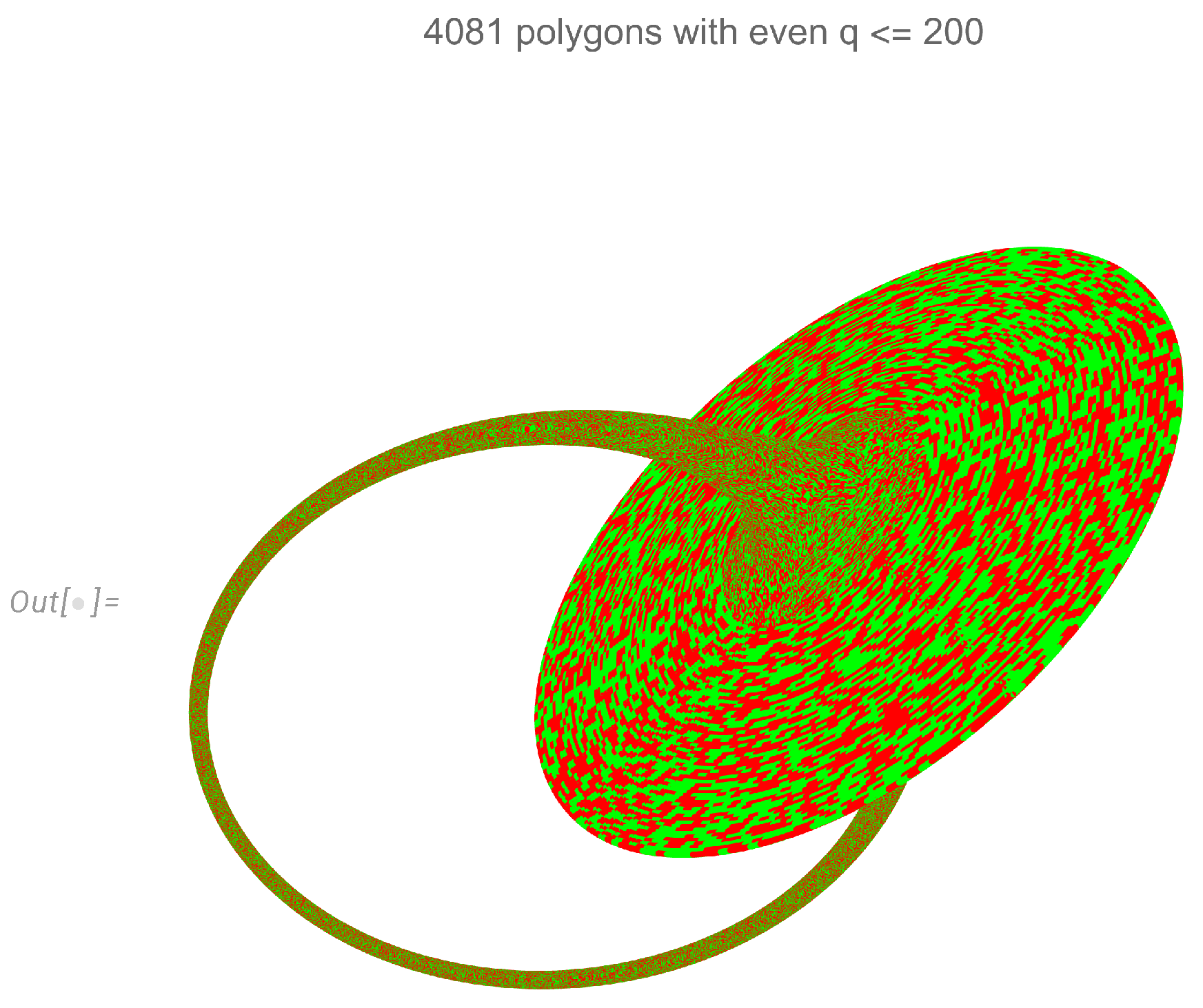
Placing these polygons for a fixed N on a torus in 3D space ordered by the angle shows the world sheet of our discrete string in Fig.Figure 4, with red/green colors of sides indicating random directions of random walk (occupation number of fermions). The large disk (infinite at ) corresponds to endpoints .
The solution of the Euler ensemble[5] is based on new number theory identities for sums of powers of cotangent of fractions of . These identities relate these sums to Jordan multi-totient functions weighted with Bernoulli coefficients.
The nontrivial part of using the Euler ensemble is the formula (84) relating this ensemble to the observable loop functional of the decaying turbulence theory.
In the string theory language, where the momentum loop is the target space along with fermionic occupation numbers, this formula is the dual amplitude for the discrete string theory, with playing the role of external momentum distributed along the closed string position (regular star polygon) .
This turbulence/string duality reveals the hidden beauty of primes under the ugly mask of chaos in the observable turbulent flow.
The corresponding universal energy spectrum for the decaying turbulence was computed in quadrature [6] in the quasiclassical limit at , and it closely matched the data of real and numerical experiments.
11.5. An Open Problem Of The Stability Of Euler Ensemble As MLE Fixed Point
The interesting and unexpected property of the Euler ensemble solution of the MLE is its independence of the spectral parameter . The dependence reappears in the linearized MLE for the small deviations from the fixed point. These deviations describe the approach of the solution of the MLE to the fixed trajectory of decaying turbulence.
As we found in the first paper [5], these deviations decay by power laws with some indexes, depending on
The spectral equation for these decay indexes was written down in [5] for the finite N in the Euler ensemble. The problem of the continuum limit of this spectrum is yet to be solved.
12. Inconsistency Of Explosive Solution
Within our dual theory, there is, in principle, a possibility for finite-time explosion with at some finite moment .
In that case, only the third-degree terms will remain on the right side, with the linear term becoming negligible at . The scale invariance fixes the time dependence in this case, so the solution becomes
The vector function must satisfy the following equation:
The left side of this equation for differs from the left side of the equation (86) for the fixed point for .
The following theorem proves the lack of a solution for this fixed point .
No explosion Theorem.
Let us assume such a solution with some vector function and arrive at a contradiction. This vector equation is a linear combination of two vectors . Both coefficients must be zero. Otherwise, these two vectors are parallel, or else one of them vanishes. In both cases, the vorticity at the loop vanishes at every point θ on the unit circle. Without vorticity, the solution reduces to the trivial fixed point .
Now, the first coefficient a can only vanish if has some imaginary component, which contradicts the requirement that the circulation is a real variable.
This requirement allows for a constant imaginary term in , as this constant term will drop in the closed loop integral. This requirement implies real discontinuity . In the explosion equation (105) with , there is no real solution with .▪
We have proven the inconsistency of the finite-time explosion in the momentum loop dynamics, i.e., the Navier-Stokes dynamics with noisy initial data and constant or vanishing velocity at infinity.
This inconsistency is a consequence of the universality and dimensional reduction of the dual fluid dynamics, leading to much more stringent conditions on a potential explosion solution, which we have proven inconsistent.
In the conventional approach to the Navier-Stokes equation, without the noise in initial data, Constantin and Fefferman have proven a theorem about the solution’s regularity [10]. As a consequence of this theorem, any singular solution must have vorticity growing to infinity at some point in time in some region in space.
In the MLE equation, vorticity at the loop would have a finite time singularity with the above hypothetical solution
In particular, the mean square of vorticity (so-called enstrophy) would have a double pole
The growth of vorticity was proven necessary for the singular solution of Navier-Stokes equation in [10], and in our theory, it is ruled out.
If proven to stay in the smooth limit , this proof would provide a negative answer to the notorious problem of the explosion in the Navier-Stokes equation, leaving two remaining alternatives: smooth (laminar) solution and a stochastic (turbulent) solution which we have found before [5,6] and reinterpreted in this work as a string theory.
Presumably, decaying turbulence occurs at a large enough Reynolds number in the initial data; otherwise, the solution stays smooth.
13. Conclusions
This work demonstrated the duality between classical incompressible fluid mechanics in Euclidean space and a nonlinear equation in loop space. Key takeaways include:
- The viscosity drops from this momentum loop equation (81), making momentum loop trajectories completely universal. The Reynolds number becomes the property of initial data , a stochastic loop in .
- There is a degenerate fixed point for covered by decaying turbulence solution: periodic random walk on a regular star polygon with steps. This fixed point (Euler ensemble) was found analytically in previous works [5,6], where the decaying energy spectrum was computed in quadrature and verified by the experimental data.
- This Euler ensemble is equivalent to a string theory with the target space made of regular star polygons. This ensemble is an explicit example of a decaying stochastic solution of the unforced Navier-Stokes equation.
- We have not proven that this solution is reachable from smooth initial data, corresponding to vanishing noise or , so we cannot claim a stochastic solution of the conventional Cauchy problem.
Acknowledgments
I benefitted from discussions of this work with Camillo de Lellis, Elia Bruè, Stan Palasek, and Jincheng Yang. Following valuable advice from Albert Schwartz, I eliminated ill-defined mathematical objects from my equations. This research was supported by the Simons Foundation award ID SFI-MPS-T-MPS-00010544 in the Institute for Advanced Study.
References
- Arnold, V. Sur la géométrie différentielle des groupes de Lie de dimension infinie et ses applications à l’hydrodynamique des fluides parfaits. Annales de l’Institut Fourier 1966, 16, 319–361. [Google Scholar] [CrossRef]
- Migdal, A. Loop Equation and Area Law in Turbulence. In Quantum Field Theory and String Theory; Baulieu, L.; Dotsenko, V.; Kazakov, V.; Windey, P., Eds.; Springer US, 1995; pp. 193–231. [CrossRef]
- Iyer, K.P.; Sreenivasan, K.R.; Yeung, P.K. Circulation in High Reynolds Number Isotropic Turbulence is a Bifractal. Phys. Rev. X 2019, 9, 041006. [Google Scholar] [CrossRef]
- Iyer, K.P.; Bharadwaj, S.S.; Sreenivasan, K.R. The area rule for circulation in three-dimensional turbulence. Proceedings of the National Academy of Sciences of the United States of America 2021, 118, e2114679118. [Google Scholar] [CrossRef] [PubMed]
- Migdal, A. To the Theory of Decaying Turbulence. Fractal and Fractional 2023, arXiv:physics.flu-dyn/2304.13719]7, 754. [Google Scholar] [CrossRef]
- Migdal, A. Quantum solution of classical turbulence: Decaying energy spectrum. Physics of Fluids 2024, 36, 095161. [Google Scholar] [CrossRef]
- Migdal, A. Statistical Equilibrium of Circulating Fluids. Physics Reports 2023, arXiv:physics.flu-dyn/2209.12312]1011C, 1–117. [Google Scholar] [CrossRef]
- Gauge Fields and Strings; Number v. 3 in Contemporary concepts in physics, Taylor & Francis, 1987.
- Bandak, D.; Mailybaev, A.A.; Eyink, G.L.; Goldenfeld, N. Spontaneous Stochasticity Amplifies Even Thermal Noise to the Largest Scales of Turbulence in a Few Eddy Turnover Times. Physical Review Letters 2024, 132. [Google Scholar] [CrossRef] [PubMed]
- Constantin, P.; Fefferman, C. Direction of Vorticity and the Problem of Global Regularity for the Navier-Stokes Equations. Indiana University Mathematics Journal 1993, 42, 775–789. [Google Scholar] [CrossRef]
| 1 | We do not count deterministic fixed points corresponding to potential flows. They correspond to isolated points on the unit circle. |
Figure 1.
Asymptotic trajectories of the time evolution for the loop functional inside the unit circle in the complex plane. The laminar flow is the yellow region on the circle close to . Three other flows are 1) hypothetical explosion, 2) decaying turbulence, and 3) special fixed point.
Figure 1.
Asymptotic trajectories of the time evolution for the loop functional inside the unit circle in the complex plane. The laminar flow is the yellow region on the circle close to . Three other flows are 1) hypothetical explosion, 2) decaying turbulence, and 3) special fixed point.
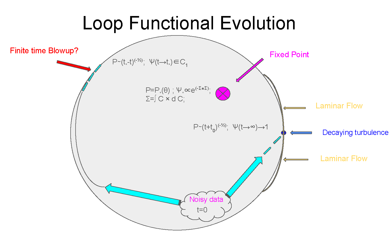
Figure 2.
The "hairpin" loop C used in defining the pair correlation of vorticity. The little circles are the loop variations needed to bring down vorticity at two points in space. The backtracking contribution to the circulation cancels at vanishing separation between these parallel lines.
Figure 2.
The "hairpin" loop C used in defining the pair correlation of vorticity. The little circles are the loop variations needed to bring down vorticity at two points in space. The backtracking contribution to the circulation cancels at vanishing separation between these parallel lines.
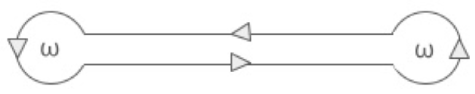
Figure 3.
regular star polygons for Euler ensembles of various . The variable indicates the direction of the random step of the link . The random walk could go several times around the polygon as long as it ends where it started.
Figure 3.
regular star polygons for Euler ensembles of various . The variable indicates the direction of the random step of the link . The random walk could go several times around the polygon as long as it ends where it started.
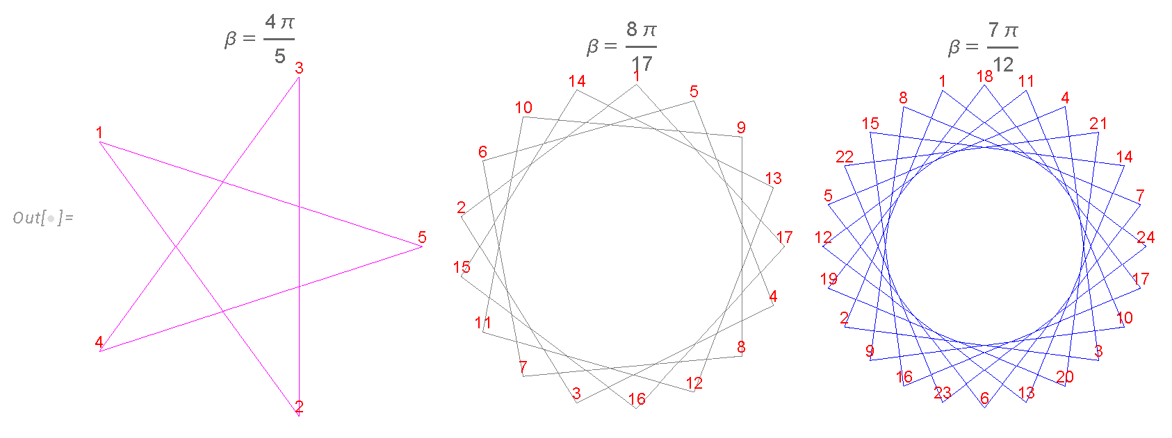
Figure 4.
The world sheet of our discrete string made of regular star polygons with unit side. The red/green colors of the sides indicate random directions of random walk.
Figure 4.
The world sheet of our discrete string made of regular star polygons with unit side. The red/green colors of the sides indicate random directions of random walk.
Disclaimer/Publisher’s Note: The statements, opinions and data contained in all publications are solely those of the individual author(s) and contributor(s) and not of MDPI and/or the editor(s). MDPI and/or the editor(s) disclaim responsibility for any injury to people or property resulting from any ideas, methods, instructions or products referred to in the content. |
© 2024 by the authors. Licensee MDPI, Basel, Switzerland. This article is an open access article distributed under the terms and conditions of the Creative Commons Attribution (CC BY) license (http://creativecommons.org/licenses/by/4.0/).
Copyright: This open access article is published under a Creative Commons CC BY 4.0 license, which permit the free download, distribution, and reuse, provided that the author and preprint are cited in any reuse.


