
Submitted:
28 October 2024
Posted:
30 October 2024
You are already at the latest version
Abstract
This chapter discusses stochastic processes known as "hidden Markov models". In these models, there are states or phases. In applications to statistical process control, for example, the states could correspond to "in control" or "out of control". In applications to the market and the economy, there are states of the market conventionally called "Bull" and "Bear", for up and down markets, resp. The states of the economy are often referred to as recession, recovery, expansion, contraction. Questions arise as to how many such states to use, and whether the nature of the states detected by statistical methods correspond to conventional notions about the phases of the market or the economy. The models considered involve a bivariate time series {Yt, St}; where Y is observed and S is the state, or label. "Hidden" means that the state is unobserved and must be inferred. For example, Yt may be the rate of return (ROR) of the S&P 500 index in month t and St may be 1 or 0, for Bull or Bear for that month. One definition of Bull and Bear is that St = 1 if the ROR Yt > 0 and St = 0; otherwise. In that case, St is directly derivable from the data. In other cases, the labels are unobserved and then are estimated from the observed process by more complicated means. The act of estimating St for each t, that is, labeling each time point of a time series with the name of its estimated state, is called time series segmentation, sequences of 0s or 1s being called segments. Thus a segment (regime, epoch) is a sequence of time points with the same label. Some definitions of phases are in terms of patterns; others are obtained in terms of fitting models in which the states are explicit elements of the model, albeit unobservable. Patterns are considered first, and then hidden state models. Use of model selection criteria for choosing between alternative models is illustrated. For example, it was found that for the stock market use of two states (corresponding to Bull and Bear) is indeed better than three states or a single state.
Keywords:
Hidden Markov Model
; Time series segmentation
| Contents | ||
| 1 | Introduction | 2 |
| 2 | Example: Bull and Bear Markets | 2 |
| 2.1 Definitions of Bull and Bear Markets................................................................................................ | 2 | |
| 2.2 Regressions on Bull3............................................................................................................... | 3 | |
| 2.2.1 Two Betas, No Alpha................................................................................................... | 3 | |
| 2.2.2 Two Betas, One Alpha.................................................................................................. | 4 | |
| 2.2.3 Two Betas, Two Alphas................................................................................................. | 5 | |
| 2.3 Other Models for Bull/Bear.......................................................................................................... | 5 | |
| 2.3.1 Two Means and Two Variances........................................................................................... | 5 | |
| 2.3.2 Mixture Model......................................................................................................... | 6 | |
| 2.3.3 Hidden Markov Model.................................................................................................. | 7 | |
| 3 | Formulation of HMMs | 8 |
| 3.1 Estimating the Parameters of an HMM................................................................................................. | 9 | |
| 3.2 More on Transition Probabilities.................................................................................................... | 9 | |
| 3.3 Bull and Bear Portfolios............................................................................................................ | 9 | |
| 4 | Example: GDP – Gross Domestic Product | 10 |
| 5 | Further Reading | 10 |
| 6 | Summary | 10 |
| 7 | References | 11 |
1. Introduction
This chapter relates to a particular type of stochastic process, namely, hidden Markov models. Markov models are defined in terms of a set of states. For example, in statistical process control, "in control" and "out of control" might be characterized by two states, with associated probability distributions. In other settings, "out of control" might be characterized by say, two states, one with a mean that is too high, the other, with a mean that is too low. We shall consider applications to finance and economics. The Markov model includes transition probabilities between states. An example of such states in the financial field is a "Bull market" and a "Bear market".
That is to say, in such applications, we speak of states or phases of the market and the economy. The states of the economy are often referred to as recession, recovery, expansion, contraction, level.
Obviously, then, questions arise as to how many such states to use, and, in the financial example, whether the nature of the states detected by statistical methods correspond to conventional notions about the phases of the market or the economy. We shall illustrate in terms of financial/economic models.
The models considered here involve a bivariate time series where Y is observed and S is the state, or label. For example, may be the rate of return of the S&P 500 index in month t and may be 1 or 0, for Bull or Bear for that month. One definition of Bull and Bear is that if the ROR and otherwise. In that case, is directly derivable from the data. In other cases, the labels are unobserved and then are estimated from the observed process by more complicated means. The act of estimating for each that is, labelling each time point of a time series with the name of its estimated state, is called time series segmentation, repeating sequences of 0s or 1s being called segments. That is, a segment (regime, epoch) is a sequence of time points with the same label. Some definitions of phases are in terms of patterns; others are obtained in terms of fitting models in which the states are explicit elements of the model, albeit unobservable ("hidden"). Patterns may be used to indicate (estimate) states, so patterns will be considered first, and then hidden state models.
2. Example: Bull and Bear Markets
2.1. Definitions of Bull and Bear Markets
The popular financial press repeats the conventional wisdom relating to the definition of Bull and Bear markets. One common definition (Vanguard Group; Investopedia) is that a Bear market is indicated by a price decline of 20% or more in a key stock market index from a recent peak over at least a two-month period. Others consider a twelve-month period. With this definition, on the average, the market is in a Bear state every four or five years. During an average Bear market, the S&P loses about 25% of its value. It usually takes 11 to 18 months for the market to hit bottom. That would be about two or three to four or five quarters, or one to one and a half years.
The simplest definition of Bull and Bear states would be to label a month as a Bear month if the market index went down in that month and as a Bull month if the market index went up in that month. This is the Up-Down (U/D) method. The U/D method definition of a Bull market indicator variable is
where is the market ROR in month t and the sign function is
If sgm( then and if sgm( then
Other definitions of Bull/Bear states can involve a moving window of, say, three months of market RORs since some analysts say that three consecutive down months of a market index constitute a Bear market. This notion can be applied to the data considered in Chapter 4. The idea is that the state should remain Bull until there are three consecutive months with negative market ROR and should remain Bear until there are three consecutive months with positive market ROR. Accordingly, define Bull3, a Bull/Bear indicator built on this idea of agreement of the most recent three months. That is, take Bull3 to be 0 (Bear) if each of the last three months had negative market ROR, equal to 1 (Bull) if each of the last three months had positive market ROR, and equals (unchanged), otherwise. That is, the Bull/Bear indicator is defined in terms of algebraically as follows.
Initialization:
- for
Computation:
- for
- if =
- if =
- otherwise.
In programming this, it is convenient to work in terms of the moving sum S3 Then if S3 if and if or 2. Table 1 at the end of the chapter shows the RORs and the Bull3 indicator.
2.2. Regressions on Bull3
Next we do some regression anaysis before going further into hidden Markov models. Some regressions on Bull3 will be shown, namely:
- two betas, no alpha: regression of fund on market and market*Bull3 (no constant)
- two betas, one alpha: regression of fund on market and market*Bull3 (with constant)
- two betas, two alphas: regression of fund on market, Bull3 and market*Bull3 (with constant)
2.2.1. Two Betas, No Alpha
This is the regression of Y = excess ROR of the fund (in percent) on excess ROR of the market and Bull3 (without a constant).

Software Output
Five years of monthly data (n = 60)
Regression Analysis:
fundROR versus marketROR, marketROR*Bull3 (marketROR times Bull3)
The regression equation is
fitted value of fundROR = 0.975 marketROR + 0.0939 marketROR*Bull3
Predictor Coef SE Coef t p
-----------------------------------------------
(No constant)
marketROR 0.97463 0.02259 43.15 0.000
marketROR*Bull3 0.09388 0.03700 2.54 0.014
s = 0.724429
Analysis of Variance
Source DF SS MS F p
--------------------------------------------------------
Regression 2 1674.80 837.40 1595.66 0.000
Residual Error 58 30.44 0.52
Total 60 1705.24
The fitted regression, of the form is
This is
The standard error of fit is (less than one percent). The variance of Y was giving
2.2.2. Two Betas, One Alpha
Next to be discussed is the model with state-dependent slope but common intercept. This is the regression of Y = excess ROR of the fund on = excess ROR of the market and Bull3 (with constant). The fitted regression will be of the form
Software Output
Regression Analysis: fundROR versus marketROR, marketROR*Bull3 \\
The regression equation is
fitted value of fundROR = 0.171 + \, 0.983 marketROR + \, 0.0729 marketROR*Bull3.
Predictor Coef SE Coef t p
---------------------------------------------------
Constant 0.17081 0.09671 1.77 0.083
marketROR 0.98350 0.02275 43.24 0.000
marketROR*Bull3 0.07286 0.03824 1.91 0.062
s = 0.711544 R-Sq = 98.3% R-Sq(adj) = 98.2%
Analysis of Variance
Source DF SS MS F p
--------------------------------------------------------
Regression 2 1676.16 838.08 1655.32 0.000
Residual Error 57 28.86 0.51
Total 59 1705.02
-------------------------------------------------------
The fitted regression is
fitted value of fundRORfund = 0.171 + 0.983 market + 0.0729 market*Bull3.
This is
fitted value of fundROR = 0.173 + 0.983 marketROR, if Bull3 = 0 = 0.173 + 1.056 marketROR, if Bull3 = 1.
The standard error of fit is 0.7115.
2.2.3. Two Betas, Two Alphas
This is the regression of Y = excess ROR of the fund on X1 = Bull3, X2 = excess ROR of the market and Bull3 (with constant), that is, the regression of ROR of the fund on the three variables ROR of the market, Bull3 and the product ROR of the market ×Bull3 (with constant).
Software Output
Regression Analysis: fundROR versus marketROR, Bull3, marketROR*Bull3
The regression equation is
fitted value of fundROR
= 0.002 + 0.975 marketROR + 0.224 Bull3 + 0.0778 marketROR*Bull3.
Predictor Coef SE Coef t p
-----------------------------------------------
Constant 0.0018 0.1957 0.01 0.993
marketROR 0.97472 0.02440 39.94 0.000
Bull3 0.2236 0.2251 0.99 0.325
marketROR*Bull3 0.07775 0.03856 2.02 0.049
s = 0.711626 R-Sq = 98.3% R-Sq(adj) = 98.2%
Analysis of Variance
Source DF SS MS F p
-------------------------------------------------
Regression 3 1676.66 558.89 1103.62 0.000
Residual Error 56 28.36 0.51
Total 59 1705.02
The fitted model is
fitted value of fundROR = 0.002 + 0.9747 marketROR + 0.224Bull3 + 0.0778 marketROR*Bull3. This is
fitted value of fund ROR = 0.002 + 0.9747 marketROR, if Bull3 = 0 = (.002 + .224) + (0.9747 + 0.0778) marketROR
= .226 + 1.0525 market, if Bull3 = 1.
The standard error of fit is 0.7116, about the same as the 0.7115 obtained with the preceding model.
2.3. Other Models for Bull/Bear
2.3.1. Two Means and Two Variances
A model with separate Bull and Bear distributions can be considered. The parameters of the two distributions can be estimated from the months with Bull3 = 0 and those with Bull3 = 1. The results are shown below. The mean and standard deviation for Bear months are mean = -3.34% and standard deviation = 7.53%; those for Bull months are mean = +0.988% and standard deviation = 3.635%, resp. Thus as expected there is a negative mean and relatively large standard deviation for Bear months and a positive mean and relatively small standard deviation for Bull months. The size of the coefficient of variation (relative standard deviation) is 7.53/3.34 = = 2.25 for Bear months and 3.635/0.988 = 3.68 for Bull months.
Descriptive Statistics: marketROR
Bull3 n Mean SE Mean StDev Min Q1 Median Q3 Max
0 16 -3.34 1.88 7.53 -18.62 -9.10 -2.42 1.03 8.96
1 44 0.988 0.548 3.635 -8.570 -0.938 1.065 3.265 8.38
The preceding is predicated upon a given indicator for Bull/Bear states. Indicators such as Bull and Bull3 seem somewhat arbitrary. What about a Bull4, based on a moving window of width 4, or a Bull2, based on a moving window of width 2? Why not use a more flexible method that lets the data do more to speak for themselves? To do this, we consider other descriptions, which model Bull and Bear as hidden (latent) states, to be detected from the data.
2.3.2. Mixture Model
Another model that incorporates hidden states and fits state-specific distributions is the finite mixture model. (See, e.g., McLachlan and Peel 2000). This model is for any number K of states and observations that may be vectors. The p.d.f. is of the form
The p.d.f.s are called component p.d.f.s. or state-conditional p.d.f.s. Sometimes the states are called classes and the corresponding distributions are called class-conditional distributions. The mixture probabilities of course must add to 1. When there are just two states, it is often convenient to index them by Then the p.d.f. is
where the mixture probabilities and add to 1. The two class-conditional distributions could be multivariate Normal. Of course, a special case is the univariate case in which the vector x is just a scalar The class-conditional densities could, for example, be Normal, with
where is the p.d.f. of the Normal distribution with mean and variance The probabilities are prior probabilities of the distributions given by and The posterior probability of state k, given x, is
In the Gaussian case this is
Denote estimates of by respectively. Estimation starts with initial guesses Then it alternates between estimating the posterior probabilities and the distributional parameters. (This alternation is an example of the EM algorithm; see Dempster, Laird and Rubin 1978; McLachlan and Krishnan 1997). At stage set the updated, stage estimates in terms of the current estimates p for states to
the updated estimates of the prior probabilities, means and variances being
where the new weights are proportional to the estimated posterior probabilities,
Iterations are continued until adequate precision is reached.
2.3.3. Hidden Markov Model
Another model with hidden (latent) states is the hidden Markov model (HMM). An HMM also consists of state-conditional probability functions, e.g., Normal distributions with different means and different variances, but in addition there is a matrix of transition probabilities. The entry of the matrix gives the probability of transition to state k, given that the process was in state j in the preceding time period,
where is the unobservable state process. Each The p.d.f. for an HMM is analogous to that of a mixture model, but with transition probabilities taking the place of mixture probabilities:
For modeling Bull and Bear states, we take and use Normal p.d.f.s, obtaining the p.d.f.
where denotes the hidden (unobservable) state, 0 for Bear, 1 for Bull, at time t.
Remarks. (i) Here, an HMM is being applied to RORs. It is often noted that the distribution of RORs is not Gaussian. Note, however, that though the marginal distribution of xt may not be Gaussian, the component densities fk(xt) in a finite mixture model or HMM may be.
(ii) In the above formulation, the transition probabilities are taken as stationary (not time-dependent, i.e., the corresponding stochastic process is homogeneous), but they may instead be modeled in terms of time-varying covariates, such as the risk-free rate. HMMs for Bull and Bear Markets. Maheu and McCurdy (2000) used a Markov-switching model that incorporates duration dependence to capture nonlinear structure in both the conditional mean and the conditional variance of stock returns. Their data are monthly returns including dividends (1802 to 1925 from Schwert 1990; 1926 to 1995:12 from CRSP, the Center for Research in Security Prices). The model sorts returns into a high-return stable state and a low-return volatile state. These can be labeled as Bull and Bear states, resp. The authors’ method identifies all major stock-market downturns in over 160 years of monthly data. Bull markets have a declining hazard function although the best market gains come at the start of a Bull market. Volatility increases with duration in Bear markets. Allowing volatility to vary with duration captures volatility clustering. According to their method the market spent 90% of the time as a Bull market and only 10% in a Bear market. Lunde and Timmermann (2004) studied time series dependence in the direction of stock prices by modeling the (instantaneous) probability that a Bull or Bear market terminates as a function of its age and a set of underlying state variables, such as interest rates. A random walk model is rejected both for bull and bear markets. Although it fits the data better, a generalized autoregressive conditional heteroscedasticity model (GARCH) is also found to be inconsistent with the very long bull markets observed in the data. The strongest effect of increasing interest rates is found to be a lower bear market hazard rate (chance of ending, as time goes on) and hence a higher likelihood of continued declines in stock prices. Huang (2011) and Huang and Sclove (2011) segmented the time series of S&P500 monthly RORs using an HMM with Gaussian p.d.f.s with differing means and variances. Three values of the number K of states were tried, With K states, the number of free parameters is means and variances and free parameters in the transition probability matrix, a total of This is 6 for 2, 12 for and just 2 for A conclusion that fits best corresponds to no state-switching and might justify fitting a single ARIMA model over all time points. A conclusion that corresponds to the conventional use of two states, Bull and Bear, particularly if one state has a positive mean ROR and the other has a negative mean. A conclusion that would suggest another state, perhaps intermediate between Bull and Bear.
BIC (Schwarz 1978) was used to compare models. is an expansion of -2 ln(posterior probability of Model k), and so can be put onto a scale of posterior probability. That is, the posterior probability of Model k is approximately proportional to exp(- (This assumes equal prior probabilities of but the expression can be adjusted for unequal prior probabilities.) That is, the posterior probability of Model k is approximately
It was found that the conventional numberr of states, K = 2, has the best (lowest) BIC and hence the highest posterior probability, with a larger variance corresponding to the Bear state.
3. Formulation of HMMs
Next the likelihood function for HMMs will be discussed.
Joint Distribution. The joint distribution of the observations in a time series may be built up from
In the case of a first order Markov process, this becomes
The joint distribution for an HMM takes account of both the observations and the hidden states. The observation vector
is Thus,
Here we have used the facts of the HMM model formulation that
and
For a given state sequence the probability is
This involves also an initial distribution The marginal distribution of the observable sequence is a sum of this over all such possible state sequences, since the event that occurs is the union of their occurrence over possible state sequences.
The Likelihood. The likelihood is the joint distribution of the observations, with the observations taken as given and the parameters taken as variables. The likelihood is to be maximized over the parameters, both the distributional parameters and the transition probabilities.
3.1. Estimating the Parameters of an HMM.
The parameters may be estimated by direct maximization of the likelihood or by iterative numerical methods such as the EM (Expectation/Maximization) algorithm; see. e.g., McLachlan and Krishnan (1997).
In the HMM model, it is natural to alternate between estimating thd distributional parameters and the transition parameters. First, make an initial guestimate of the states. For example, in the case of a scalar observation and two states, estimate low values as State 1 and high values as State 2. Then estimate the distributional parameters by method of moments, or maximum likelihood (giving an EM algorithm). Then, for time given that relabel according to arg Then re-estimate the distributional parameters. Etc.
A special case of the EM algorithm is the Baum-Welch algorithm (Baum and Welch; Baum, Petrie, Soules and Weiss 1970). In the Baum, Petrie, Soules and Weiss article (1970), there is a reference to a paper by Baum and Welch submitted to the Proceedings of the National Academic of Sciences (PNAS), but the archives of PNAS reveal no publication by Baum and Welch. The Baum-Welch algorithm has become an important tool in many fields, first especially in speech recognition. The algorithm estimates the probability distribution over the states of the hidden Markov chain at each time point. Though formulated before any general formulation of the EM algorithm, the Baum-Welch algorithm is an EM algorithm. We do not elaborate further on the Baum-Welch algorithm here. For further discussion of it, see, e.g., McLachlan and Krishnan (1997).
3.2. More on Transition Probabilities
As above, let These are the transition probabilities. The process is homogeneous if these are constant across time. The transition probability matrix is The distribution across states at time t is the vector where S is the number of states. Then to move forward one time period, T
Having estimated the transition probabilities, one may solve for the steady-state, long run distribution across the states. If is the transition probabilty matrix and is the steady-state distribution, then to find , one solves the set of simultaneous linear equations i.e., which is the homogeneous set of equations
3.3. Bull and Bear Portfolios
Having segmented the relevant time series of market indicators into states such as Bull and Bear, one may then estimate the mean vector and covariance matrix of a portfolio of selected stocks and form an optimal Bull portfolio and an optimal Bear portfolio. The estimate of an optimal weight vector is a function of the estimate of the mean vector and of the covariance matrix, say There are estimates and for Bull and Bear states, resp.;
One would try to predict whether or not there will be a change in the state of the market, and rebalance or not, accordingly. A decision risk analysis should be performed to see if the expected increase in portfolio ROR would compensate for transaction costs incurred in rebalancing. The transaction costs might be proportional to the amount of buying and selling across the m stocks, that is, proportional to where is the weight of asset a in the portfolio for state
4. Example: GDP – Gross Domestic Product
Next, a macro-economic example, GDP, will be considered further. Gross domestic product is the total monetary or market value of all the finished goods and services produced within the country’s borders in a specific time period. GDP is similar to GNP (Gross National Product), except the GNP includes imports and exports, whereas GDP excludes them. This modeling could be applied to GNP as well.
In terms of time series analysis, a seasonal ARIMA model for, say, log quarterly GDP could be discussed. It is interesting to compare this with a model with different states, although even if it happened that a single ARIMA model fit better, one might still want to fit a model with states, which labels the time points. Chen and Sclove (2011) fit a state model to GDP. The time series of quarterly growth rates of US GDP, from 1947 through the third quarter of 2010, was segmented by hidden Markov models (HMMs). HMMs with several states were fit and compared with a single distribution for the growth rate. State-conditional Normal distributions with different means and variances were fit for different numbers of states. The extent to which states correspond to recession, recovery, expansion, and contraction was assessed. The HMMs were scored by BIC (Schwarz 1978). Some comparison was made to ARIMA models involving regular and quarterly differencing and regular and quarterly autoregression of log GDP. Components of GDP were also fit with HMMs, with a view toward determining which components are leading or lagging indicators of the state of overall GDP.
5. Further Reading
The model selection criterion BIC was formulated by Schwarz (1978); the paper by Kashyap (1982) is also very helpful. To begin a study of HMMs, it is helpful to begin with the Viterbi algorithm, which finds the most likely state sequence. See Viterbi (1968) and Forney (1978). Then for further study on the HMM, one may refer, for example, to McLachlan and Krishnan (1997) or Zucchini and MacDonald (2009) or Zucchini, MacDonald and Langrock (2016).
6. Summary
Stochastic processes, such as time series, may have states. These are phases through which the process passes over time. Examples are Bull and Bear states of the stock market, and Recession, Recovery, Expansion, and Contraction in the economy. A segment (regime, epoch) is a sequence of time points having the same state. Segmentation involves labeling each time point with its most likely state, or giving a probability distribution over the states for each time point.
Hidden Markov models involve state-conditional p.d.f.s and transitions between states, with the corresponding transition probabilities. The state process is a Markov chain with a transition probability matrix. Alternative, competing models with different numbers of states and different state-conditional distributions can be compared with criteria such as BIC (Bayesian Information Criterion). The values of BIC for the alternative models can be put on a scale of posterior probability.
References
- Baum, Leonard E., and Welch, Lloyd (ca. 1970). A statistical estimation procedure for probabilistic functions of finite Markov processes. Submitted for publication to Proceeding of the National Academy of Sciences, U.S.A.
- Baum, L. E.; Petrie, T.; Soules, G.; Weiss, N. A maximization technique occurring in the statistical analysis of probabilistic functions of Markov chains. Annals of Mathematical Statistics 1970, 41, 164–171. [Google Scholar] [CrossRef]
- Chen, Y.; Sclove, S.L. Segmenting the time series of quarterly GDP using a hidden Markov model. Presentation at the Joint Statistical Meetings (American Statistical Association and related societies), Miami Beach, FL.
- Dempster, A. P.; Laird, N. M.; Rubin, D. B. Maximum likelihood from incomplete data via the EM algorithm. Journal of the Royal Statistical Society, Series B (Methodological) 1977, 39, 1–38. [Google Scholar] [CrossRef]
- Forney, G. D. The Viterbi algorithm. Proceedings of the IEEE 1973, 61, 268–278. [Google Scholar] [CrossRef]
- Huang, Z. Segmentation of financial and marketing data: mixture logit model and hidden Markov model. PhD dissertation, Department of Information & Decision Sciences, University of Illinois Chicago, 2011. [Google Scholar]
- Huang, Z.; Sclove, S. L. Segmenting the time series of a market index using a hidden Markov model. Working Paper, Dept. of Information & Decision Sciences, University of Illinois at Chicago, 2011. [Google Scholar]
- Investopedia (2011). Bear market.www.investopedia.com/terms/b/bearmarket.asp#axzz1gXPbjeE2.
- Kashyap, R.L. Optimal choice of AR and MA parts in autoregressive moving average models. IEEE Transactions on Pattern Analysis and Machine Intelligence 1982, 4, 99–104. [Google Scholar] [CrossRef]
- Lunde, A.; Timmermann, A. Duration dependence in stock prices: an analysis of Bull and Bear markets. Journal of Business and Economic Statistics, 2004, 22, 253–273. [Google Scholar] [CrossRef]
- Maheu, J.M.; McCurdy, T.H. Identifying Bull and Bear markets in stock returns. Journal of Business and Economic Statistics 2000, 18, 100–112. [Google Scholar] [CrossRef]
- McLachlan, G.; Krishnan, T. The EM Algorithm and Extensions; Wiley: New York, 1997. [Google Scholar]
- McLachlan, G.; Peel, D. McLachlan, Geoffrey, and Peel, David (2000). In Finite Mixture Models; Wiley: New York.
- Schwarz, G. Estimating the dimension of a model. Annals of Statistics 1978, 6, 461–464. [Google Scholar] [CrossRef]
- Schwert, G. W. Indexes of U.S. stock prices from 1802 to 1987. Journal of Business 1990, 63, 399–426. [Google Scholar] [CrossRef]
- Vangard Group (2011). Staying calm during a Bear market.retirementplans.vanguard.com/VGApp/pe/PubVgiNews?
- Viterbi, A. J. Error bounds for convolutional codes and an asymptotically optimum decoding algorithm. IEEE Transactions on Information Theory 1967, 13, 260–269. [Google Scholar] [CrossRef]
- Zucchini, W.; MacDonald, I.L. Hidden Markov Models for Time Series: an Introduction using R; Chapman & Hall/CRC (Taylor & Francis Group): Boca Raton, FL, 2009. [Google Scholar]
- Zucchini, W.; MacDonald, I.L.; Langrock, R. Hidden Markov Models for Time Series: An Introduction Using R, 2nd ed.; Chapman & Hall/CRC (Taylor & Francis Group): Boca Raton, FL.

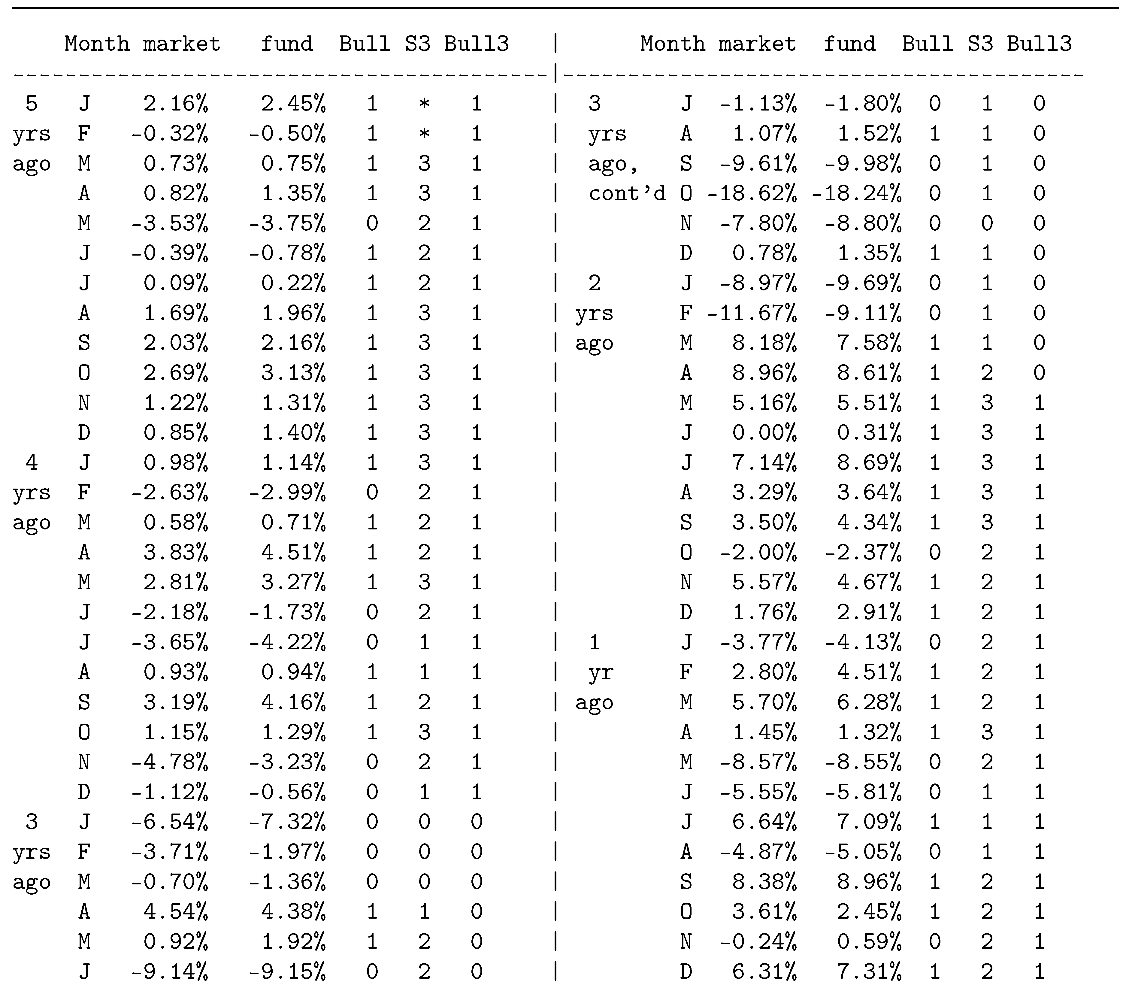
Table 1.
Excess monthly RORs (%) of market and fund, with Bull/Bear state defined as Bull3. S3 is the moving sum of 3.
Table 1.
Excess monthly RORs (%) of market and fund, with Bull/Bear state defined as Bull3. S3 is the moving sum of 3.
Disclaimer/Publisher’s Note: The statements, opinions and data contained in all publications are solely those of the individual author(s) and contributor(s) and not of MDPI and/or the editor(s). MDPI and/or the editor(s) disclaim responsibility for any injury to people or property resulting from any ideas, methods, instructions or products referred to in the content. |
© 2024 by the authors. Licensee MDPI, Basel, Switzerland. This article is an open access article distributed under the terms and conditions of the Creative Commons Attribution (CC BY) license (http://creativecommons.org/licenses/by/4.0/).
Copyright: This open access article is published under a Creative Commons CC BY 4.0 license, which permit the free download, distribution, and reuse, provided that the author and preprint are cited in any reuse.


