
Submitted:
28 October 2024
Posted:
30 October 2024
You are already at the latest version
Abstract
Floating offshore wind turbine (FOWT) systems are advancing quickly, but they still need to become economically viable for large-scale commercial adoption. Design optimization is essential for reaching this objective by reducing costs while ensuring the best possible system performance and structural integrity. The present study aims to carry a comparative multi objective optimization (MOO) of a 10MW FOWT semisubmersible using three different metaheuristic optimizations technics and sophisticated approach for optimizing a floating concept through the utilization of global limit states. The optimization is performed in Python, integrating PyMAPDL and PyMOO for intricate modeling and simulation tasks. The ZJUS10 floating offshore wind turbine (FOWT) platform, developed by the state key laboratory of wind power at Zhejiang University, is employed as the basis for this study. Key criteria, such as platform stability, overall structural mass, and the stress, are pivotal in formulating the objective functions. Based on a preliminary study the three Metaheuristic Optimization Algorithms chosen for optimization are Particle Swarm Optimization (PSO), Simulated Annealing (SA), and Ant Colony Optimization (ACO). Then, the solutions are evaluated based on Pareto dominance, leading to a Pareto front, a curve that represents the best possible trade-offs among the objectives. Each algorithm's convergence is meticulously evaluated, leading to the selection of the optimal design solution. The results evaluated in simulations elucidate the strengths and limitations of each optimization method, providing valuable insights into their efficacy for complex engineering design challenges. In the post-processing phase, the performance of the optimized FOWT platforms is thoroughly compared both among themselves and with the original model, resulting in validation and endorsement.
Keywords:
Renewable Energy
; Floating Offshore Wind Turbine
; Metaheuristic
; Evolutionary Algorithms
; Particle Swarm Optimization
; Ant Colony Analysis
; Simulated Annealing
1. Introduction
The increasing global demand for renewable energy has led to significant advancements in offshore wind technology[1,2]. Floating Offshore Wind Turbines (FOWTs) have emerged as a viable solution for deep-water installations, where wind speeds are higher and traditional fixed-bottom turbines are impractical[3]. FOWTs offer several advantages over onshore and nearshore wind turbines, including reduced noise and increased energy production[4,5]. Among the various floating platform designs, semisubmersibles are favored in mainland China due to their inherent stability in deep waters and cost-effectiveness[6]. However, installing FOWTs is more challenging because of the high construction costs and the need for more advanced offshore wind farm technology[7,8]. The commercialization and competitiveness of these platforms[9] consider three main factors: cost-effectiveness, stability in deeper waters, and structural integrity. Optimizing these three parameters is a complex task that requires balancing multiple objectives. Recent advances in Multi Objective Optimization (MOO) have focused on Metaheuristic[10,11] approaches that combine machine learning techniques that enhance the performance of optimization algorithms[12,13].
Evolutionary Algorithms (EAs) remain the most prevalent techniques in the world of metaheuristics, especially in the optimization of Floating Offshore Wind Turbines (FOWTs). Jiazhi Wang et al. (2024) [14] presents a multi-objective optimization framework for the design of a 15 MW semi-submersible floating offshore wind turbine using an evolutionary algorithm. T.A. Boghdady et al. (2016) [15] introduces an innovative hybrid evolutionary algorithm, LBBO-DE (Linearized Biogeography-Based Optimization and Differential Evolution), for maximizing power generation in wind energy conversion systems (WECS). Furthermore, Hüseyin Hakli et al. (2019) [16] proposes a modified differential evolution (MDE) algorithm for solving the wind turbine placement problem. Serhat Duman et al. (2021) develops the Multi-Objective Adaptive Guided Differential Evolution (MO-AGDE) algorithm, applied to optimize the multi-objective AC optimal power flow (MO-ACOPF) for hybrid energy sources, including wind, photovoltaic (PV), and tidal systems. Christos A. Christodoulou (2020) et al. [17] applies the Harmony Search Method to estimate the optimal number of wind turbines in a wind farm. Ramazan Özkan et al. (2023) [18] investigates the aerodynamic design and optimization of small-scale wind turbine blades using a novel artificial bee colony algorithm based on blade element momentum (ABC-BEM) theory. Ajay Sharma et al. (2021) [19] focuses on the design of controller parameters for a wind turbine emulator using an artificial bee colony algorithm. Besides, Oussama Maroufi et al. (2020) [20] introduces a hybrid fractional fuzzy PID controller for Maximum Power Point Tracking (MPPT) and pitch control of wind turbines. In terms of real-time optimization, Su, Yongxin. et al. (2017) .[21] tackled the challenge of balancing power production and fatigue loads in wind turbines by developing a method that handles real-time optimization. Charhouni et al. (2019) [22] took a different angle, focusing on reducing the Levelized Cost of Energy (LCOE) in wind farms.
While this study focuses on metaheuristic technics, it specifically delves into Ant Colony Optimization (ACO), Particle Swarm Optimization (PSO), and Simulated Annealing (SA), all of which do not belong to the Evolutionary Algorithms (EAs) family. In this hand Kyoungboo Yang (2019)[23] proposed a novel layout optimization method for wind farms using the Simulated Annealing (SA) algorithm.. Similarly, A. Mu (2022) [24] focused on floating wind turbines and introduced an optimal model reference adaptive control (MRAC) approach, optimized with Simulated Annealing. Peng Chen (2021) [25]applied the Simulated Annealing algorithm to predict the dynamic response of floating offshore wind turbines (FOWTs). On a similar note, Yongman Park (2015)[26] focused on optimizing the hull form of semi-submersible Floating Production Units (FPUs). Ruilin Chen (2024)[27] developed an improved SA algorithm to optimize the electrical collector systems in large offshore wind farms.
Additionally, Xiaoqiang Wen (2020) brought together Ant Colony Optimization (ACO) with the Extreme Learning Machine (ELM) to model and evaluate wind turbine performance. Similarly, Mahmudur Rahman (2019) [28] used Ant Colony Optimization (ACO) to model and control wind turbine tower vibrations. Xiaoqiang Wen (2020)[29] combined ACO with the Extreme Learning Machine (ELM) to further improve wind turbine performance prediction. Yunus Eroğlu (2019) [30] took a fresh approach to fault detection in wind turbines by using an artificial neural network (ANN) trained with a novel ACO-based algorithm, Antrain ANN. Similarly, Xin Zhao (2023) [31] explored the optimal sizing of hybrid energy storage for wind power systems using ACO.
Further, Gu, B et al. (2021) [32]developed an efficient method for maximizing power output in small- and medium-scale wind farms using Particle Swarm Optimization (PSO). Tang et al. (2022) [33]introduced a hybrid optimization method to lower the Levelized Cost of Energy (LCOE) in wind farms. In a similar vein, Song et al. (2023)[34] combined PSO with the Arithmetic Optimization Algorithm (AO) to minimize construction and power loss costs. Yong Ma et al. (2019) [35] explored how PSO, combined with the FAST program, could optimize offshore wind turbine blade design. Jianping Zhang (2022) [36] applied an improved PSO algorithm alongside a Back Propagation Neural Network (BPNN) to assess offshore wind resources in China.
This paper explores a multi-objective optimization of a 10MW semisubmersible aiming to reach a better stability of the FOWT system, a reduced mass and optimal structural integrity. Starting with a detailed look at the ZJUS10 floating platform which covers essential topics like hydrodynamics, aerodynamics, mooring dynamics, and the coupled dynamic analysis method. In Section 2, the optimization problem is clearly defined, and the paper discusses the chosen optimization approach, optimizer, and the specific settings and processes involved. Section 3 focuses on how the results are selected and analyzed in depth.
2. ZJUS10 Platform Optimization Methodology
2.1. ZJUS10 FOWT System
2.1.1. ZJUS10 Floating Platform
The Floating Offshore Wind Turbine (FOWT) typically comprises the wind turbine, the floating platform, and the mooring system. In this paper, the whole FOWT is regarded as a rigid body. According to Newton’s second law, its dynamic equations of motions in the time domain is as follows:
where represents the inertia of the whole system.
This study established that the primary stability requirements of the FOWT system include maintaining a maximum pitch angle of less than 10°. Additionally, the area enclosed by the system’s restoring moment curve up to the immersion angle must be at least 130% of that enclosed by the tilting moment curve. Concerning the motion response criteria, the acceleration at the top of the tower should not exceed 1.5 m/s². Moreover, the period of oscillatory motion should ideally fall outside the wave period range of the selected maritime area. The 10 MW FOWT semi-submersible investigated in this work (Figure 1), named ZJUS10[37,38], which employs the DTU10MW wind turbine designed by the Technical University of Denmark, with a rated wind speed of 11.4 m/s. The tower stands at 103 meters and has a natural frequency exceeding 0.5 Hz, categorizing it as a rigid body. The ZJUS10 semi-submersible platform was developed by our research team of Zhejiang University, featuring a compact and straightforward design that uses concrete and water for ballast[38,39]. The Y-shaped pontoons are crucial for ensuring buoyancy and stability. A Cartesian coordinate system featuring XYZ axes, which are customarily employed in similar applications was employed situating the origin at (0, 0, 0), positioned at the mean free surface at the midpoint of the mid-column. Within this framework, the Z-axis extends vertically upward, while the X-axis is oriented in the direction of wave incidence. The origin remains consistently anchored at the center of gravity (COG) and adapts in accordance with any transitions or rotations of the floating body. The design also provides uniform has a draft of 22 meters and a freeboard of 16 meters, with a submerged volume of 257,900 cubic meters, including the pontoons, cones, and 4 meters of the cylinder height. The Y-shaped pontoons are essential for buoyancy and stability, while the column size influences the platform’s response to wave loading and its ability to support the wind turbine. The mooring system is symmetrically configured with three catenary lines to constrain the platform’s movement in six degrees of freedom. The ZJUS10 is intended for operation at a water depth of 130 meters.

Table 1.
Dimensions of the ZJUS10 platform.
| Parameter | Value |
| Draft | 22 |
| Airgap | 12 |
| H _c2_up | 16 |
| H_c2 _mid | 12 |
| H_c2_down | 6 |
| D_c1_up | 14 |
| D_c1_mid | 16 |
| D_c1_down | 16 |
| ac | 69 |
| Width, d | 10 |
| Rod diameter, r | 3 |
Figure 1.
ZJUS10 platform and coordinates system.
2.1.2. 10 MW Wind Turbine
Aerodynamic loads on blades are calculated based on the blade element momentum (BEM) theory[40], where blades are divided into many small elements that act as two-dimensional airfoils. For each blade element, the generated axial forces can be expressed as:
Which represents the air density, and represents the lift coefficient and the drag coefficient respectively, represents the inflow angle, C represents the blade element chord, Vrel represents the relative incoming flow velocity between the air and the blade element cross-section, and can be expressed as:
represents the incoming wind speed, represents the rotation speed of the rotor, and represents the axial induction factor and tangential induction factor respectively. Besides, several nonlinear unsteady aerodynamic effects of tip losses, hub losses, dynamic inflow and skewed wake are considered based on related empirical correction methods.
Figure 2.
The aerodynamic loads of a blade element.
Shown in Table 2, the rotor diameter of such a turbine typically ranges from 170 to 220 meters. The blades, which can exceed 90 meters in length, are meticulously crafted to maximize wind energy capture. The expansive rotor diameter allows the turbine to sweep a larger area, thereby enhancing the energy harvested from the wind. The hub height of a 10MW wind turbine generally stands between 100 to 150 meters above ground level. The cut-in wind speed, the minimum speed at which the turbine begins generating power, is typically around 3 to 4 meters per second (m/s). Conversely, the cut-out wind speed, the maximum speed at which the turbine can safely operate, usually lies between 25 to 30 m/s. The rated wind speed, at which the turbine achieves its maximum power output of 10MW, typically falls within the range of 12 to 14 m/s.
The numerical model of the 10 MW FOWT was constructed in FAST software shown in Figure 3, and the time domain simulation analysis was carried out at the designed steady conditions with the uniform wind speed of 11.4 m/s speed and regular wave height of 2.5 m height and 10 s period.
2.1.3. Catenary Mooring System
The mooring system employed in this study successfully maintained the ZJUS10 at a height of 326 meters and with a rope strength of 305 meters. It operates by leveraging the inherent weight and length of the mooring lines to provide stability and ensure the platform remains anchored in its designated position.
Table 3.
Coordinates of the used catenary mooring system.
| Parameter | Value |
| Equivalent mass(in air) | 375 kg/m |
| Equivalent mass(in water) | 3200 N/m |
| Extensional stiffness(EA) | 1.51e9 N |
| Added mass coefficient | 0.8 |
| Damping coefficient | 2.0 |
| Catenary diameter | 0.137 m |
| Pretension | 1.67e6 N |
Illustrated in Figure 4, the catenary curve of the lines imparts stability through both horizontal and vertical components of tension. The weight of the mooring lines exerts a downward force, while their length and tension generate horizontal forces[41]. The horizontal restoring force counteracts the lateral displacement of the floating platform induced by wind, waves, and currents, whereas the vertical forces arise from the combined effects of the mooring line’s weight and the buoyancy of the floating structure. The catenary mooring system applied on the ZJUS10 was analyzed in AQWA as shown in Figure 5 considering quasi static and Coupled dynamics. Considering the mooring line weight, seabed friction, and nonlinear restoring forces of the catenaries, the mooring line tensions can be calculated by the quasi-static equilibrium and dynamic method [42] and expressed as:
where represents the pretensions of the mooring system in its undisplaced position. represents the linearized restoring matrix of the mooring system and is the combined result of the elastic stiffness and the effective geometric stiffness brought by the weight of the mooring lines in water.
2.2. ZJUS10 System Analysis in Ansys
2.2.1. Coupled Dynamic Analysis
The principal objective of the ZJUS10 analysis in AQWA is to assess stability. Initially, hydrostatic tilting was evaluated, with specific focus on the pitch and roll angles, which were computed using the restoring matrix. The hydrostatic stiffness matrix delineates the restoring forces and moments exerted on the ZJUS10 as a result of displacements in heave, roll, pitch, and other degrees of freedom.
The equations of motion for pitch and roll are derived from the restoring moments and can be expressed as:
is the moment of inertia about the pitch axis. the hydrostatic stiffness coefficient for pitch. the hydrostatic stiffness coefficient for roll. is the external moment applied to the structure.
The hydrodynamic analysis in AQWA adopts a Fully Coupled analysis approach, integrating interactions among the wind turbine, the floating platform, and mooring system.
The simulation was divided into three case studies: the first case study focuses on hydrodynamic diffraction analysis, where the wave environment is defined by several intermediate wave directions, with eight specific directions spaced at 45-degree intervals, as depicted in the Figure 6a. For the results Figure 6c,d it was only considered beam seas waves (90degree) instead of head seas (0 degree). The goal was also the evaluate the roll inclination as head sea waves will be the main consideration in hydrodynamic response. The wave heights reached up to 3 meters and periods varied between 0 and 15 seconds, although typical wave periods in the East and South China Sea are generally between 0 and 20 seconds. The wave excitation forces on the structure are calculated by AQWA, they entail determining the potential flow around the semi-submersible and analyzing wave scattering and diffraction effects.
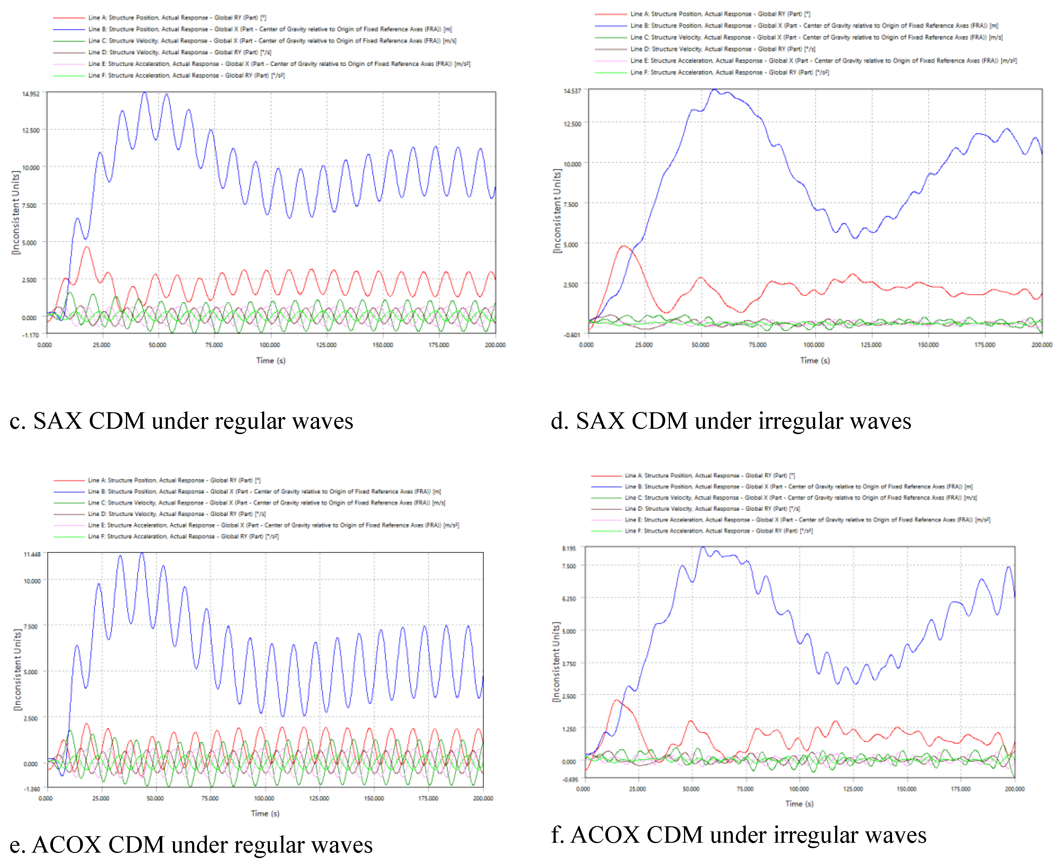
In the second case study, the analysis extends to hydrodynamic response under regular waves Figure 6b, utilizing a time step of 0.1 seconds over a total duration of 100 seconds. A regular wave height of 3 meters was considered, and the mooring system was modeled with a catenary load Figure 5, characterized by a stiffness (EA) of 1,506,000 kN and a maximum anticipated tension of 5,000 kN. Wind force of 1.615e6 max amplitude previous calculated on FAST. Figure 3 were and incorporated into the evaluation of the maximum pitch inclination angle.
For the third case study Figure 6b the setup was modified to include an Irregular Wave Spectrum based on the JONSWAP spectrum, while maintaining the same conditions. This setup featured a wave direction of 0 degrees, a peak period of 10 seconds, a spectral index of γ = 2.3, and a wave height of 3 meters.
The results, as depicted in the Figure 6c–h, analyzed in hydrodynamic diffraction the Response Amplitude Operator RAO, which quantifies the relationship between wave amplitude (input) and the structure’s response amplitude (output). As the wave angle increases, the pitch angle also rises, with rotations Ry and Rx showing slightly larger pitch and roll displacements compared to Rz. The pitch, roll, and yaw are synchronized with the wave action, causing the platform to move in harmony with the waves. In hydrodynamic response under a variety of wave conditions, the system is inclination more stable under regular wave conditions than irregular ones. The maximum pitch displacement was calculated through iterative step response and actual equilibrium position response while accounting for the aerodynamic loads of the floating wind turbine, resulted in an estimated pitch rotation of 5.6 degrees. The roll and yaw displacements are relatively smaller.
2.2.2. Structural Integrity Analysis
Then ANSYS Static Structural is used to evaluate the stress of the platform under the hydrodynamic loads calculated from AQWA imported as boundary conditions. The results post-processed to evaluate maximum stresses, identify the pontons as critical high stress points with a maximum von-mises stress reaching up to 2.2e8, as illustrated in Figure 7. The reason of the high stress is the hydrodynamic analysis in AQWA might be conducted for extreme sea states, leading to higher-than-usual loads. The increased stress observed on the pontoons after importing hydrodynamic pressure data from AQWA is primarily due to the complex interaction between hydrodynamic loads, structural responses, and potential modeling differences.
2.2.3. ZJUS10 Sensitivity Analysis
The sensitivity analysis performed in Python, using relative sensitivity based on finite difference method to adjust for the scale of X and Y [43,44] demonstrated that the pontoons and the wide have a substantial impact on the structure. Sensitivity analysis is an essential technique for obtaining deeper insights into model dynamics. As depicted in Figure 8, the mass and pitch of the semisubmersible are primarily influenced by the pontoons and conical towers. However, the columns play a pivotal role in affecting stress distribution. The findings from this sensitivity analysis provide crucial information that can be leveraged in the development of optimization algorithms.
Where is a small change in the input and is the corresponding change in the output
2.3. Problem Definition Optimization Objectives
Along with the simulation done in AQWA to evaluate the stability of the platform, an experiment was done in (Zhejiang Province of China) after testing manufacturing and testing, Figure 9. In this experiment, a geometric Froude scaling[45] factor of 1:50 is employed, resulting in a correspondingly scaled platform structure. Concrete is pre-installed internally as fixed ballast, while cross-shaped metal structures are utilized to mitigate the movement of ballast water. The tower, standing at a height of 2.07 meters, is securely bolted to the central pontoon. Instead of the rotor, an actuation system is implemented, comprising fans, aluminum alloy cantilevers, motors, and controllers. The wave basin spans 70 meters in length, 40 meters in width, and has a depth of 1.5 meters, with a maximum operational water depth of 1 meter. The wave period varies between 0.3 and 5.0 seconds, and the wave height ranges from 0.03 to 0.3 meters. However, during pool trials, it was observed that the semi-submersible platform exhibited unexpected pitch instability. The platform’s tilt along its horizontal axis, became more pronounced than anticipated, leading to concerns about the platform’s overall stability.
The weight of floating offshore wind turbine (FOWT) semi-submersibles is a critical factor influencing their performance, cost, and overall feasibility. However, the ZJUS10 platform has a mass (including structure and ballast) of 24,052,000 kg, which even exceeds that of the DTU10. Reducing the weight of semi-submersible FOWTs has significant implications for the levelized cost of energy (LCOE), a key metric in assessing the economic viability of wind energy projects. Moreover, managing stress is crucial to ensuring the long-term structural integrity of a semi-submersible platform. A stress level of 2.25e8 Pa approaches the maximum yield stress of the high strength steel, highlighting the platform’s vulnerability. Thus, the three primary challenges facing our current platform are excessive mass, stability concerns, and structural integrity. The triple objective function is defined as :
where represents the stability criteria, the mass, and the structural integrity.
The parameters chosen for optimization, as shown in Table 4, were selected based on a sensitivity analysis of the ZJUS10 model, established engineering practices for numerical calculations, and industry standards. Both the design variables and the global limit state criteria are restricted by specific bounds. These limits were defined through sensitivity analysis and previous simulations and experiments with the ZJUS10 model, taking into account key factors: , , (with ); α ) The setup of these constraints is primarily influenced by the goal of reaching a wider stochastic search, the significance of the parameters and the necessity of preserving the structural integrity of the model’s shape.
2.4. Optimization Methodology and Optimizers
The optimization process for the ZJUS10 floating platform involves three main tasks. First, Python is used to integrate numerical values and the Finite Element Analysis (FEA) model in PyMapdl with metaheuristic optimization algorithms from the Pymoo library. Python computes the mass and pitch angle based on coordinates and floating offshore wind turbine dynamics, while PyMapdl calculates mechanical stress. The Pymoo library is used to run optimization algorithms like PSO, ACO, and SA to analyze convergence behavior. The second task involves hydrodynamic analyses in AQWA. The third task includes experimental validation in a laboratory to verify platform stability. The results for mass, pitch angle, and stress after optimization are compared to the original platform’s metrics.
Figure 10.
Optimization Methodology.
This work explored the strength of the ZJUS10 by computing is stress using the command mapdl.stress. The primary reason for utilizing PyAnsys in our work is to import the stress data of the ZJUS10 into our optimization solver. By integrating PyMapdl with others python libraries for optimization, we harnessed the power of MAPDL simulations within the optimization framework, allowing for the automatic exploration of design spaces and the identification of optimal solutions. After the 3D plot of the ZJUS10 the mass in is computed based on the material properties, volume, and density of the elements within the model. The command was then used for quick calculation of the mass. Then right after getting the mass of the ZJUS10, the hydrostatic picth is calculated based on the structure mass and the hydrostatic stiffness coefficient C55 which is derived from the stiffness matrix.
Figure 11.
ZJUS10 stress FEA and stress computation in PyMapdl.
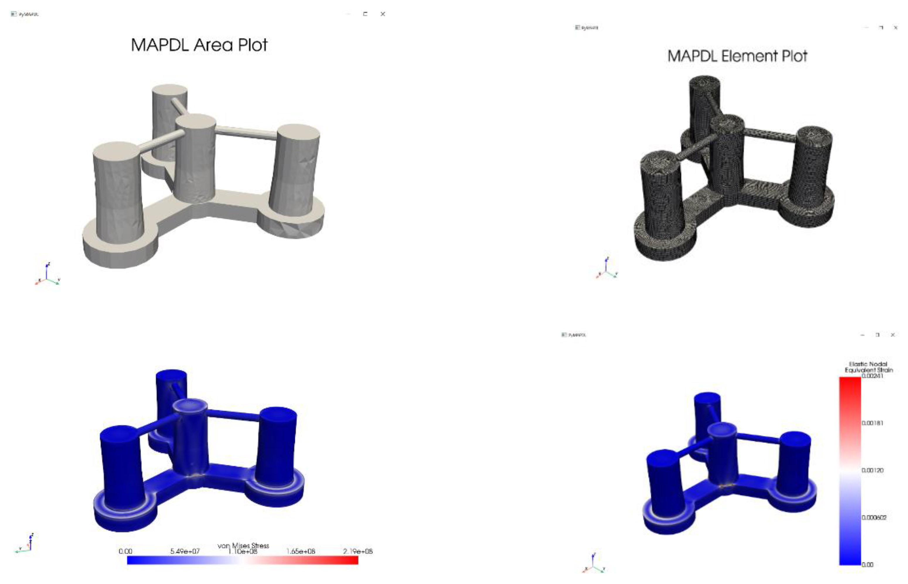
As mention above, PyMoo was chosen as the primary solver due to its capability to integrate seamlessly with other Python libraries such as PyMapdl, NumPy, and SciPy. This Pymoo code which can encompass NSGA-II, SA, MOEA/D, PSO, ACO was developed based on reference codes from the School of Mechatronics at Zhejiang University and additional resources from GitHub. The ZJUS10 optimization process leverages the minimize function from PyMoo, invoked as “from pymoo.optimize import minimize,” with the objective of achieving minimization for each of the objective functions[46]. The objective function incorporated terms for f1, f2, and f3 with constraints to guarantee feasible designs. The chosen optimizers for this work are PSO, ACO, SA.
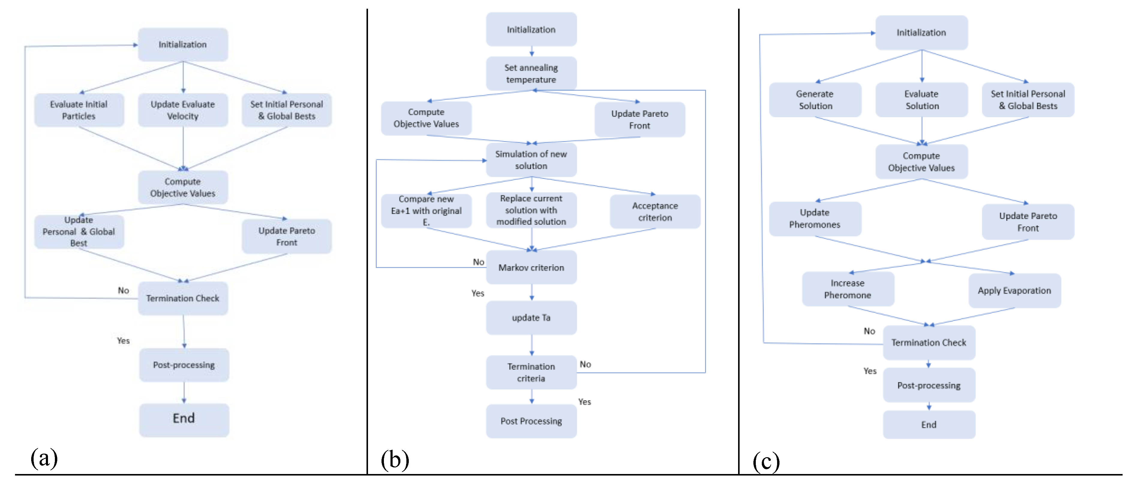
The first, PSO algorithm code was the initial implementation using the Pymoo open-source framework[47]. Inspired by the social behavior of bird flocks, the algorithm optimizes a problem by iteratively improving candidate solutions based on their own experience and that of their neighbors[48,49]. Each particle adjusts its velocity and position according to specific equations (18,19) and a flow chart (Figure 12).
where (t) is the position of particle at time t and (t+1) the updated velocity of particle
where (t): Velocity of particle iii at time t, ω: Inertia weight. c1, c2: Cognitive and social acceleration coefficients, respectively. r1 , r2: Random numbers uniformly distributed in [0,1]. then (t): Best known position of particle i (personal best) and(t): global best.
Simulated Annealing (SA) draws inspiration from the annealing process in metallurgy, Figure 12, where controlled cooling of a material reduces defects[50,51]. The algorithm explores the solution space by accepting or rejecting new solutions based on a probability that decreases with temperature over time. The temperature T governs the likelihood of accepting worse solutions as the algorithm advances.
Where T0 represents the initial temperature, α is the cooling rate (0 < α < 1), k is the current iteration and change in energy.
The semi-submersible parameters in ACO are constructed based on pheromone levels and heuristic information. The key idea in ACO is the use of pheromone trails, which guide the search process based on the experiences of previous iterations[52,53], illustrated in the following equations and flow chart in Figure 12. The probability of an ant choosing a path is influenced by the intensity of the pheromone trail and the heuristic desirability of the path. In this study we updated the pheromone levels based on the quality of the solutions found by the ants. Then Combine the components into the main loop of the ACO algorithm. The evaporation reduces the pheromone levels to avoid premature convergence.
Where Q is the Constant representing the total amount of pheromone deposited and the Length of the path traveled by ant.
Where m is the Number of ants, the Pheromone deposited by ant k on edge (i,j) the Pheromone level on edge (i,j) at time t. ρ the Pheromone evaporation rate (0 < ρ < 1). the Amount of pheromone deposited on edge (i,j) by ants.
Where : Probability that ant k will move from node iii to node j at time t. α the Parameter to control the influence of pheromone. β the Parameter to control the influence of heuristic information the Heuristic information. the Set of neighbors of node i.
Figure 12.
flow charts of PSO(a), SA(b), ACO(c) [54].
Figure 12.
flow charts of PSO(a), SA(b), ACO(c) [54].
3. Results and Discussion
The Pymoo-based PSO optimization code included 1,000 particles and a total of 700 iterations. The inertia weight (w) was set to 0.5, with the cognitive and social coefficients chosen as c1=1 and c2=2. Then SA began with an initial solution with parameters and an initial temperature T0 = 1000. The number of iterations also set at 700, involved repeating the following steps until the system had sufficiently “cooled.” The cooling rate, or alpha, was set at 0.5. The algorithm terminates when the temperature reaches a sufficiently low level, after a fixed number of iterations. About ACO, the number of ants was chosen as 1000. Then the number of iterations 700 as the others. Besides evaporation rate ρ 0.5 then the importance of pheromone α 1.0 and the importance of heuristic β 2.0. The data were meticulously selected according to the ACO methodology described earlier, incorporating the essential computational formulas central to ACO: pheromone updating and the probabilistic determination of the next node.
Throughout the iterations, PSO tends to have faster convergence and continuously tracks the best solution found by any particle (global best) as well as the best solution found by each individual particle (personal best). The particles are continuously pulled toward the best-known positions, both personal and global. Once particles find promising areas of the solution space, they rapidly refine their positions, leading to faster optimization in many cases and reaching the optimal result after 12h and only required 87 iterations.
The initial high temperature in SA (T0) was crucial and influenced the algorithm’s exploration of the solution space. Its high value allows the algorithm to accept worse solutions like higher energy states, with a greater probability, thereby facilitating exploration and preventing the algorithm from getting trapped in local optima. Each iteration evaluated one new solution at a time against the current solution: As the temperature decreases, the probability of accepting worse solutions also decreased. The best result was found at iteration 286th Iteration with 26h of running time and is the outcome of the best solution found during the entire annealing process.
ACO algorithm stored the best solution at each iteration when it improves upon the previous best. It was noticed that the ACO code took take longer to converge. It’s no doubt due to the fact it often requires several iterations for pheromones to accumulate and guide ants toward the best regions of the solution space. In addition, the convergence speed was also influenced by factors like the evaporation rate, which controls how quickly pheromone trails decay. The best solution was found 42h after starting at a later iteration: 431th and remains the best through subsequent iterations.
The optimized parameters results provided by the three algorithms were illustrated in Table 5. Besides the minimized objectives functions minimal values were highlighted in Table 6. The 3D pareto plots Figure 13 revealed a cloud of solutions with various trade-offs, helping to illustrate the complex interdependencies between objectives. The solutions at the corners typically indicate extreme trade-offs where one or more objectives are being maximized or minimized to their fullest extent. The solution considered f1 for selection and decision making as it’s the most critical objective in order to provide a good balance of smaller pitch, and mass while also being relatively low in stress distribution. The mass is also sensitive, but its effects are less immediate compared to those of the pitch angle. The pitch angle of the ZJUS10 system is more sensitive because it directly affects the system structural loading. Shown in Table 6 and Figure 14, the SAX is the widest platform among the three, followed by PSOX, which has a more compact triangular configuration footprint is more compact compared to ZJUS10, though it remains wider than ACOX. This wide configuration provides significant stability by distributing the platform’s weight and buoyancy over a large area.
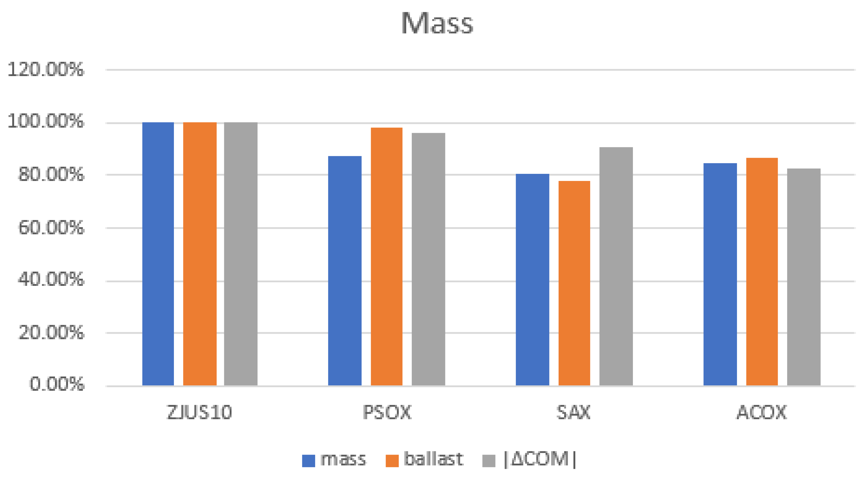
3.1. Mass Analysis
By incorporating various constraints and applying the ZJUS10 mass calculation formula, the results of the optimization indicate that the most streamlined platform achieves a total weight of 19,251,984.52 kg. This reflects a significant reduction of 19.79% from the original mass of the ZJUS10, evidencing a highly successful optimization outcome. Both ACOX and SAX configurations demonstrate a lowered center of mass, with vertical displacements of ∆z -4m and -3m from the original, respectively. This is achieved by strategically concentrating mass in the lower sections of their structures, thereby markedly enhancing stability and reducing the platform’s susceptibility to tilting under wind and wave forces. Furthermore, the buoyant columns generate a righting moment that further fortifies stability. The ACO’s center of buoyancy is meticulously positioned to maximize stability through an extended righting arm. The ACOX configuration strikes an astute balance between the necessary displacement for stability and the flexibility required for diverse operational conditions, while maintaining a substantial submerged volume, thereby increasing the displaced volume.
Figure 15.
mass evaluation.
3.2. Stress Analysis
PyMAPDL was utilized to evaluate the comparative stress distribution across different platform designs. The maximum stress remained concentrated on the pontoons, particularly at the connection points, which are subjected to the highest stress levels, Figure 16. Although the reduction in maximum stress was not huge, it still decreased to less than the original value. Notably, the stress concentration regions expanded significantly around the longitudinal pontoon in all three models. The SAX model exhibited higher stress levels compared to the PSOX and ACOX models, though it still represents 93.1% of the original ZJUS10 stress. This is largely due to the SAX model’s lower center of gravity and increased submerged volume. Conversely, the PSOX model experienced stress levels at 91.8% of the original, which, while lower, remained higher than those in the ACOX model which stands at 87.3%. Additionally, elevated stress concentrations were observed at critical points, including the junction between the center column and the upper horizontal brace, as well as the connection between the outer column and the diagonal brace. The structural integrity of the frame at the base of the outer column is vital for maintaining strength, and wave loads further exacerbate stress levels near the tower base.
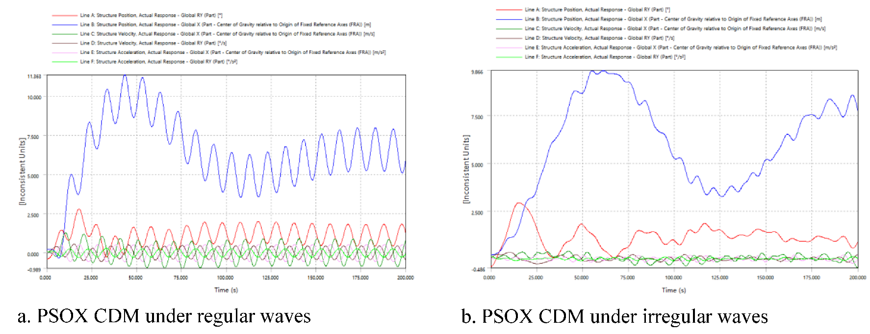
3.3. Hydrodynamic Analysis
Hydrodynamic diffraction analysis reveals that SAX exhibits a slightly higher RAO-based displacement compared to PSOX and ACOX, yet its maximum rotational motions are significantly Higher. The optimized models demonstrate out-of-phase degrees of freedom, potentially reducing the overall tilt of the platform and thereby enhancing stability. The pitch time history calculations under operational conditions indicate that the maximum inclination angles for PSOX, SAX, and ACOX under dynamic loads, as evaluated in AQWA, are considerably smaller than those of the original model. The ACOX model achieves the most optimal hydrodynamic pitch angle at 2.3 degrees, as shown below. PSOX’s deep draft and ballast confer exceptional stability, particularly in pitch and yaw. Meanwhile, SAX enhances stability through its distributed buoyancy and structural rigidity. ACOX’s design, featuring higher heave plates, a low center of gravity, and a broad footprint, also offers superior stability. The current stability results suggest that a smaller hydrostatic pitch angle corresponds to a smaller hydrodynamic pitch angle, thereby affirming the initial hypothesis. A reduced hydrostatic pitch angle indicates a design with a lower center of gravity or improved weight distribution, which enhances the platform’s natural frequency and damping characteristics.
Figure 17.
Stability Analysis.
6. Conclusion
In this paper, a multi optimization approach is presented and applied to the ZJUS10 semi-submersible FOWT system to reduce mass, inclination and ensure better structural integrity. Starting with the reference system and its implementation for being simulated in FAST, AQWA and PyMAPDL. Processing these for the formal description of the optimization problem. Then proceeded a substantiated selection and specification of the optimization variables and global limit states and the integration of three metaheuristic algorithms (PSO, SA, ACO) to the PyMoo framework for automated simulation and optimization. Finishing off with the final selection approach of the optimum and its evaluation, then a comparison with the initial model, and validation of results using PyMAPDL and AQWA. PSO demonstrated rapid convergence, often reaching near-optimal solutions within fewer iterations compared to SA and ACO. ACO was the most robust algorithm, consistently yielding good solutions in repeated trials. It also showed better performance in exploring complex regions of the search space, potentially finding higher-quality solutions over more extended iterations. The ACO optimization achieved a best optimum reduction of 19.8% in weight, 40.1% in pitching, 12.7% in stress compared to the original model, thereby providing significant support for LOCE, AEP, and other engineering applications. The optimization concept presented in this paper surpasses the limitations of its current application, providing a versatile approach for optimizing engineering structures and demonstrating promising avenues for future development. These results and the presented methodologies serve as basis for further in depth and more sophisticated application of the design optimization approach, including local criteria, integrity checks, fatigue analyses, as well as reliability aspects.
Author contributions
Drabo Souleymane: Writing – original draft, Visualization, Data curation, Methodology; Lai Siqi: Data curation, Methodology; Xiangheng Feng: Conceptualization; Lui Hongwei: Project administration, Supervision
Data availability
The data that support the findings of this study are available from the corresponding author upon reasonable request.
Acknowledgements
This research was funded by the National Natural Science Foundation of China (U22A20178), Science and Technology Project of Zhejiang Province (2023C01123), Basic Public Welfare Research Program of Zhejiang Province (LHZ21E090004) and Natural Science Foundation of Zhejiang Province (LY22E090001), National Natural Science Foundation of China (No. 52275070).
Declaration of Competing Interest
The authors declare that they have no known competing financial interests or personal relationships that could have appeared to influence the work reported in this paper.
References
- Sun, X.; Huang, D.; Wu, G. The current state of offshore wind energy technology development. Energy 2012, 41, 298–312. [Google Scholar] [CrossRef]
- Kaldellis, J.; Kapsali, M. Shifting towards offshore wind energy—Recent activity and future development. Energy policy 2013, 53, 136–148. [Google Scholar] [CrossRef]
- Díaz, H.; Soares, C.G. Review of the current status, technology and future trends of offshore wind farms. Ocean Engineering 2020, 209, 107381. [Google Scholar] [CrossRef]
- Barooni, M.; Ashuri, T.; Velioglu Sogut, D.; Wood, S.; Ghaderpour Taleghani, S. Floating offshore wind turbines: Current status and future prospects. Energies 2022, 16, 2. [Google Scholar] [CrossRef]
- Ha, K.; Truong, H.V.A.; Dang, T.D.; Ahn, K.K. Recent control technologies for floating offshore wind energy system: A review. International Journal of Precision Engineering and Manufacturing-Green Technology 2021, 8, 281–301. [Google Scholar] [CrossRef]
- Qiao, D.; Ou, J. Global responses analysis of a semi-submersible platform with different mooring models in South China Sea. Ships and Offshore Structures 2013, 8, 441–456. [Google Scholar] [CrossRef]
- Chitteth Ramachandran, R.; Desmond, C.; Judge, F.; Serraris, J.-J.; Murphy, J. Floating wind turbines: marine operations challenges and opportunities. Wind Energy Science 2022, 7, 903–924. [Google Scholar] [CrossRef]
- Asim, T.; Islam, S.Z.; Hemmati, A.; Khalid, M.S.U. A review of recent advancements in offshore wind turbine technology. Energies 2022, 15, 579. [Google Scholar] [CrossRef]
- Díaz, H.; Serna, J.; Nieto, J.; Guedes Soares, C. Market needs, opportunities and barriers for the floating wind industry. Journal of Marine Science and Engineering 2022, 10, 934. [Google Scholar] [CrossRef]
- Abdel-Basset, M.; Abdel-Fatah, L.; Sangaiah, A.K. Metaheuristic algorithms: A comprehensive review. Computational intelligence for multimedia big data on the cloud with engineering applications 2018, 185–231. [Google Scholar]
- Minguijón, D.H.; Pérez-Rúa, J.-A.; Das, K.; Cutululis, N.A. Metaheuristic-based design and optimization of offshore wind farms collection systems. Proceedings of 2019 IEEE Milan PowerTech; pp. 1–6.
- Karl, F.; Pielok, T.; Moosbauer, J.; Pfisterer, F.; Coors, S.; Binder, M.; Schneider, L.; Thomas, J.; Richter, J.; Lang, M. Multi-objective hyperparameter optimization in machine learning—An overview. ACM Transactions on Evolutionary Learning and Optimization 2023, 3, 1–50. [Google Scholar] [CrossRef]
- Morales-Hernández, A.; Van Nieuwenhuyse, I.; Rojas Gonzalez, S. A survey on multi-objective hyperparameter optimization algorithms for machine learning. Artificial Intelligence Review 2023, 56, 8043–8093. [Google Scholar] [CrossRef]
- Wang, J.; Ren, Y.; Shi, W.; Collu, M.; Venugopal, V.; Li, X. Multi-objective optimization design for a 15 MW semisubmersible floating offshore wind turbine using evolutionary algorithm. Applied Energy 2025, 377, 124533. [Google Scholar] [CrossRef]
- Boghdady, T.; Sayed, M.; Elzahab, E.A. Maximization of generated power from wind energy conversion system using a new evolutionary algorithm. Renewable energy 2016, 99, 631–646. [Google Scholar] [CrossRef]
- Hakli, H. A new approach for wind turbine placement problem using modified differential evolution algorithm. Turkish Journal of Electrical Engineering and Computer Sciences 2019, 27, 4659–4672. [Google Scholar] [CrossRef]
- Christodoulou, C.A.; Vita, V.; Seritan, G.-C.; Ekonomou, L. A harmony search method for the estimation of the optimum number of wind turbines in a wind farm. Energies 2020, 13, 2777. [Google Scholar] [CrossRef]
- Özkan, R.; Genç, M.S. Aerodynamic design and optimization of a small-scale wind turbine blade using a novel artificial bee colony algorithm based on blade element momentum (ABC-BEM) theory. Energy Conversion and Management 2023, 283, 116937. [Google Scholar] [CrossRef]
- Sharma, A.; Sharma, H.; Khandelwal, A.; Sharma, N. Designing controller parameter of wind turbine emulator using artificial bee colony algorithm. In Proceedings of Intelligent Learning for Computer Vision: Proceedings of Congress on Intelligent Systems 2020; pp. 143–151.
- Maroufi, O.; Choucha, A.; Chaib, L. Hybrid fractional fuzzy PID design for MPPT-pitch control of wind turbine-based bat algorithm. Electrical Engineering 2020, 102, 2149–2160. [Google Scholar] [CrossRef]
- Su, Y.; Li, Q.; Duan, B.; Wu, Y.; Tan, M.; Qiao, H. A coordinative optimization method of active power and fatigue distribution in onshore wind farms. International transactions on electrical energy systems 2017, 27, e2392. [Google Scholar] [CrossRef]
- Charhouni, N.; Sallaou, M.; Mansouri, K. Realistic wind farm design layout optimization with different wind turbines types. International Journal of Energy and Environmental Engineering 2019, 10, 307–318. [Google Scholar] [CrossRef]
- Yang, K.; Cho, K. Simulated annealing algorithm for wind farm layout optimization: A benchmark study. Energies 2019, 12, 4403. [Google Scholar] [CrossRef]
- Mu, A.; Huang, Z.; Liu, A.; Wang, J.; Yang, B.; Qian, Y. Optimal model reference adaptive control of spar-type floating wind turbine based on simulated annealing algorithm. Ocean Engineering 2022, 255, 111474. [Google Scholar] [CrossRef]
- Chen, P.; Song, L.; Chen, J.-h.; Hu, Z. Simulation annealing diagnosis algorithm method for optimized forecast of the dynamic response of floating offshore wind turbines. Journal of Hydrodynamics 2021, 33, 216–225. [Google Scholar] [CrossRef]
- Park, Y.; Jang, B.-S.; Du Kim, J. Hull-form optimization of semi-submersible FPU considering seakeeping capability and structural weight. Ocean engineering 2015, 104, 714–724. [Google Scholar] [CrossRef]
- Chen, R.; Zhang, Z.; Hu, J.; Zhao, L.; Li, C.; Zhang, X. Grouping-based optimal design of collector system topology for a large-scale offshore wind farm by improved simulated annealing. Protection and Control of Modern Power Systems 2024, 9, 94–111. [Google Scholar] [CrossRef]
- Rahman, M.; Ong, Z.C.; Chong, W.T.; Julai, S.; Ng, X.W. Wind turbine tower modeling and vibration control under different types of loads using ant colony optimized PID controller. Arabian Journal for Science and Engineering 2019, 44, 707–720. [Google Scholar] [CrossRef]
- Wen, X. Modeling and performance evaluation of wind turbine based on ant colony optimization-extreme learning machine. Applied Soft Computing 2020, 94, 106476. [Google Scholar] [CrossRef]
- Eroğlu, Y.; Seçkiner, S.U. Early fault prediction of a wind turbine using a novel ANN training algorithm based on ant colony optimization. Journal of Energy Systems 2019, 3, 139–147. [Google Scholar] [CrossRef]
- Zhao, X. Optimal allocation of wind power hybrid energy storage capacity based on ant colony optimization algorithm. Engineering Optimization 2024, 1–17. [Google Scholar] [CrossRef]
- Gu, B.; Meng, H.; Ge, M.; Zhang, H.; Liu, X. Cooperative multiagent optimization method for wind farm power delivery maximization. Energy 2021, 233, 121076. [Google Scholar] [CrossRef]
- Tang, X.-Y.; Yang, Q.; Stoevesandt, B.; Sun, Y. Optimization of wind farm layout with optimum coordination of turbine cooperations. Computers & Industrial Engineering 2022, 164, 107880. [Google Scholar]
- Song, D.; Shen, G.; Huang, C.; Huang, Q.; Yang, J.; Dong, M.; Joo, Y.H.; Duić, N. Review on the application of artificial intelligence methods in the control and design of offshore wind power systems. Journal of marine science and engineering 2024, 12, 424. [Google Scholar] [CrossRef]
- Ma, Y.; Zhang, A.; Yang, L.; Hu, C.; Bai, Y. Investigation on optimization design of offshore wind turbine blades based on particle swarm optimization. Energies 2019, 12, 1972. [Google Scholar] [CrossRef]
- Zhang, J.; Zhu, Y.; Chen, D. Assessment of offshore wind resources, based on improved particle swarm optimization. Applied Sciences 2022, 13, 51. [Google Scholar] [CrossRef]
- Feng, X.; Lin, Y.; Gu, Y.; Li, D.; Chen, B.; Liu, H.; Sun, Y. Preliminary stability design method and hybrid experimental validation of a floating platform for 10 MW wind turbine. Ocean Engineering 2023, 285, 115401. [Google Scholar] [CrossRef]
- Feng, X.; Lin, Y.; Gu, Y.; Zhao, X.; Liu, H.; Sun, Y. Indirect load measurement method and experimental verification of floating offshore wind turbine. Ocean Engineering 2024, 303, 117734. [Google Scholar] [CrossRef]
- Feng, X.; Huang, P.; Lin, Y. The hybrid model test of floating offshore wind turbine based on an aerodynamic actuation system. Proceedings of International Joint Conference on Civil and Marine Engineering (JCCME 2023); p. 6.
- Dorrego-Portela, J.R.; Ponce-Martínez, A.E.; Pérez-Chaltell, E.; Peña-Antonio, J.; Mateos-Mendoza, C.A.; Robles-Ocampo, J.B.; Sevilla-Camacho, P.Y.; Aviles, M.; Rodríguez-Reséndiz, J. Angle Calculus-Based Thrust Force Determination on the Blades of a 10 kW Wind Turbine. Technologies 2024, 12, 22. [Google Scholar] [CrossRef]
- Rocha, M.; Schnaid, F.; Rocha, C.; Amaral, C. Inverse catenary load attenuation along embedded ground chain of mooring lines. Ocean Engineering 2016, 122, 215–226. [Google Scholar] [CrossRef]
- Azcona, J.; Munduate, X.; González, L.; Nygaard, T.A. Experimental validation of a dynamic mooring lines code with tension and motion measurements of a submerged chain. Ocean Engineering 2017, 129, 415–427. [Google Scholar] [CrossRef]
- Iooss, B.; Saltelli, A. Introduction to sensitivity analysis. Handbook of uncertainty quantification 2017, 1103–1122. [Google Scholar]
- Saltelli, A.; Annoni, P. Sensitivity Analysis. 2011.
- Bredmose, H.; Lemmer, F.; Borg, M.; Pegalajar-Jurado, A.; Mikkelsen, R.F.; Larsen, T.S.; Fjelstrup, T.; Yu, W.; Lomholt, A.K.; Boehm, L. The Triple Spar campaign: Model tests of a 10MW floating wind turbine with waves, wind and pitch control. Energy procedia 2017, 137, 58–76. [Google Scholar] [CrossRef]
- Blank, J.; Deb, K. Pymoo: Multi-Objective Optimization in Python. IEEE Access 2020, 8, 89497–89509. [Google Scholar] [CrossRef]
- pso. Availabe online: https://github (accessed.
- Kennedy, J.; Eberhart, R. Particle swarm optimization. In Proceedings of Proceedings of ICNN'95-international conference on neural networks; pp. 1942–1948.
- Shami, T.M.; El-Saleh, A.A.; Alswaitti, M.; Al-Tashi, Q.; Summakieh, M.A.; Mirjalili, S. Particle swarm optimization: A comprehensive survey. Ieee Access 2022, 10, 10031–10061. [Google Scholar] [CrossRef]
- Delahaye, D.; Chaimatanan, S.; Mongeau, M. Simulated annealing: From basics to applications. Handbook of metaheuristics 2019, 1–35. [Google Scholar]
- Guilmeau, T.; Chouzenoux, E.; Elvira, V. Simulated annealing: A review and a new scheme. Proceedings of 2021 IEEE statistical signal processing workshop (SSP); pp. 101–105.
- Dorigo, M.; Stützle, T. Ant colony optimization: overview and recent advances; Springer: 2019.
- Dorigo, M.; Birattari, M.; Stutzle, T. Ant colony optimization. IEEE computational intelligence magazine 2006, 1, 28–39. [Google Scholar] [CrossRef]
- Chopard, B.; Tomassini, M.; Chopard, B.; Tomassini, M. Simulated annealing. An introduction to metaheuristics for optimization 2018, 59–79. [Google Scholar]
Figure 3.
ZJS10 Fowt system Aerodynamics analysis.
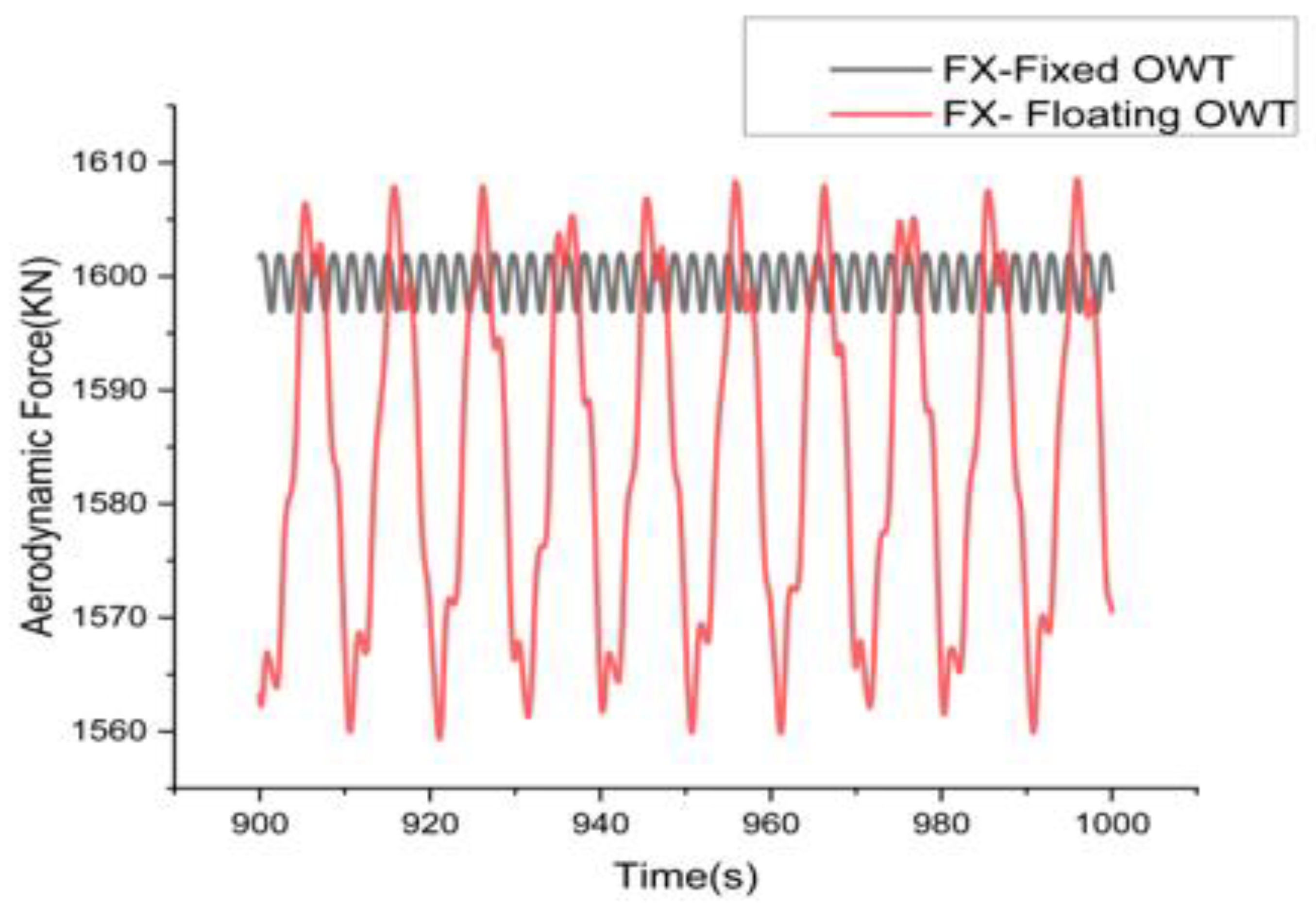
Figure 4.
ZJUS10 catenary mooring system.
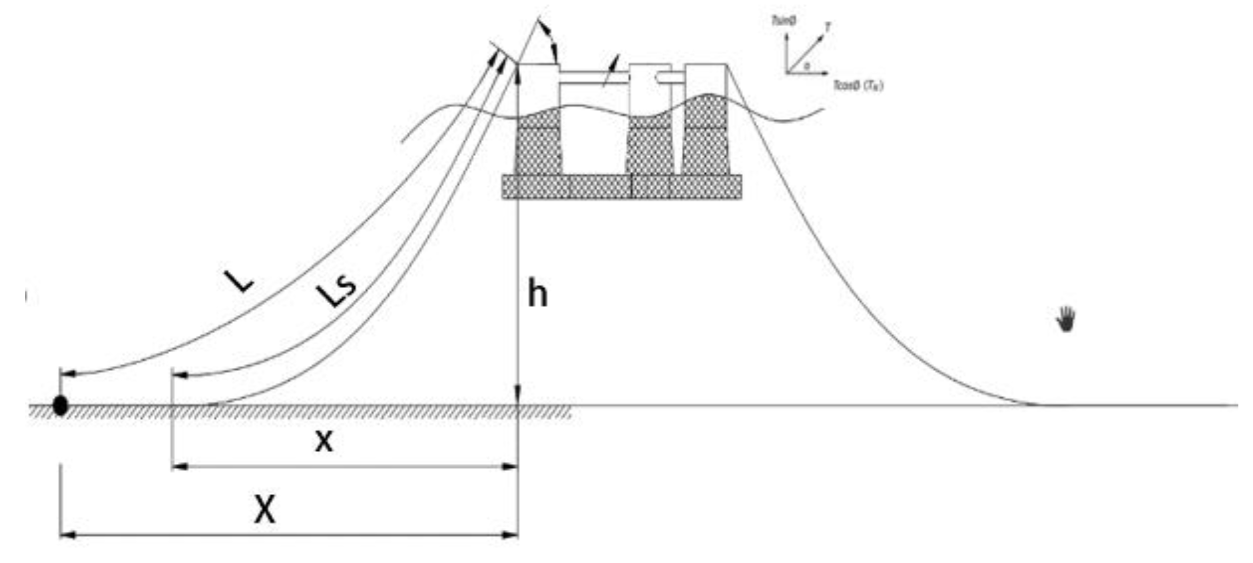
Figure 5.
Mooring loads analysis from AQWA.
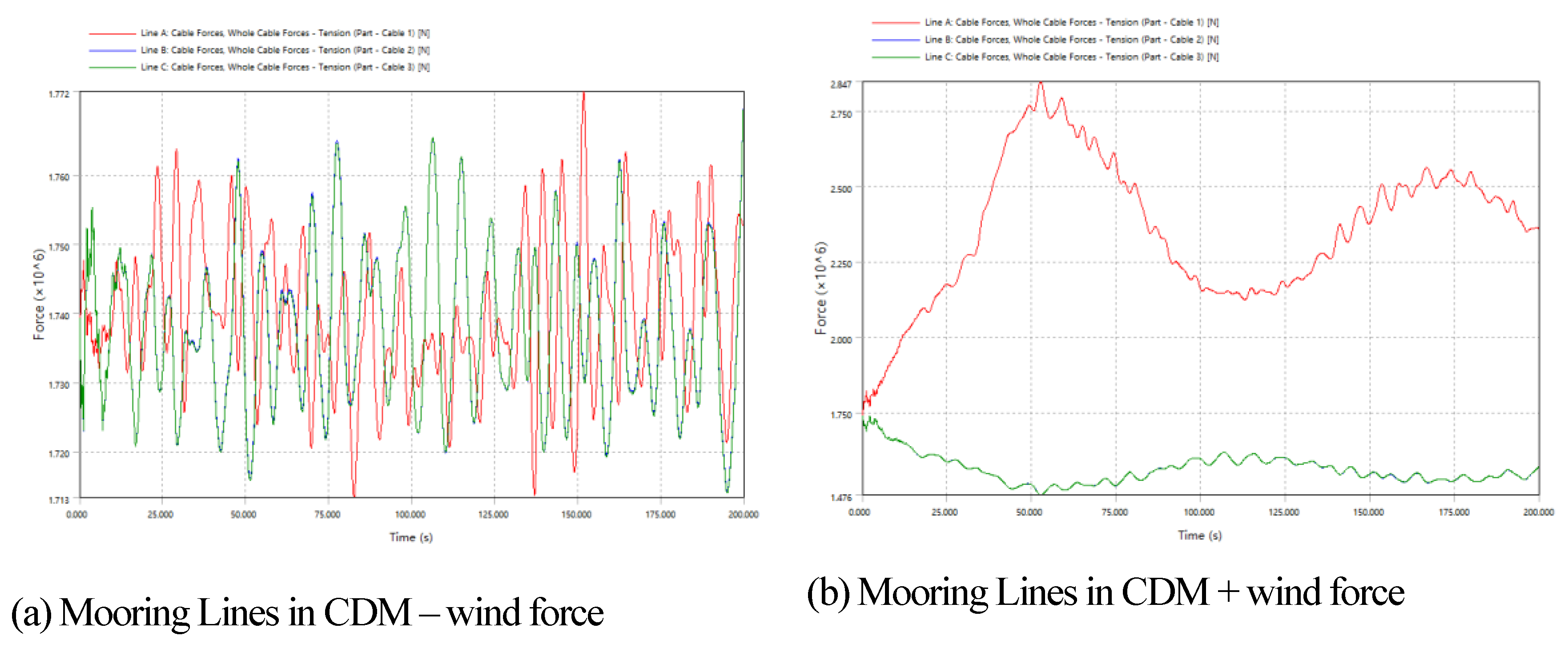
Figure 6.
Hydrodynamic diffraction and response AQWA.
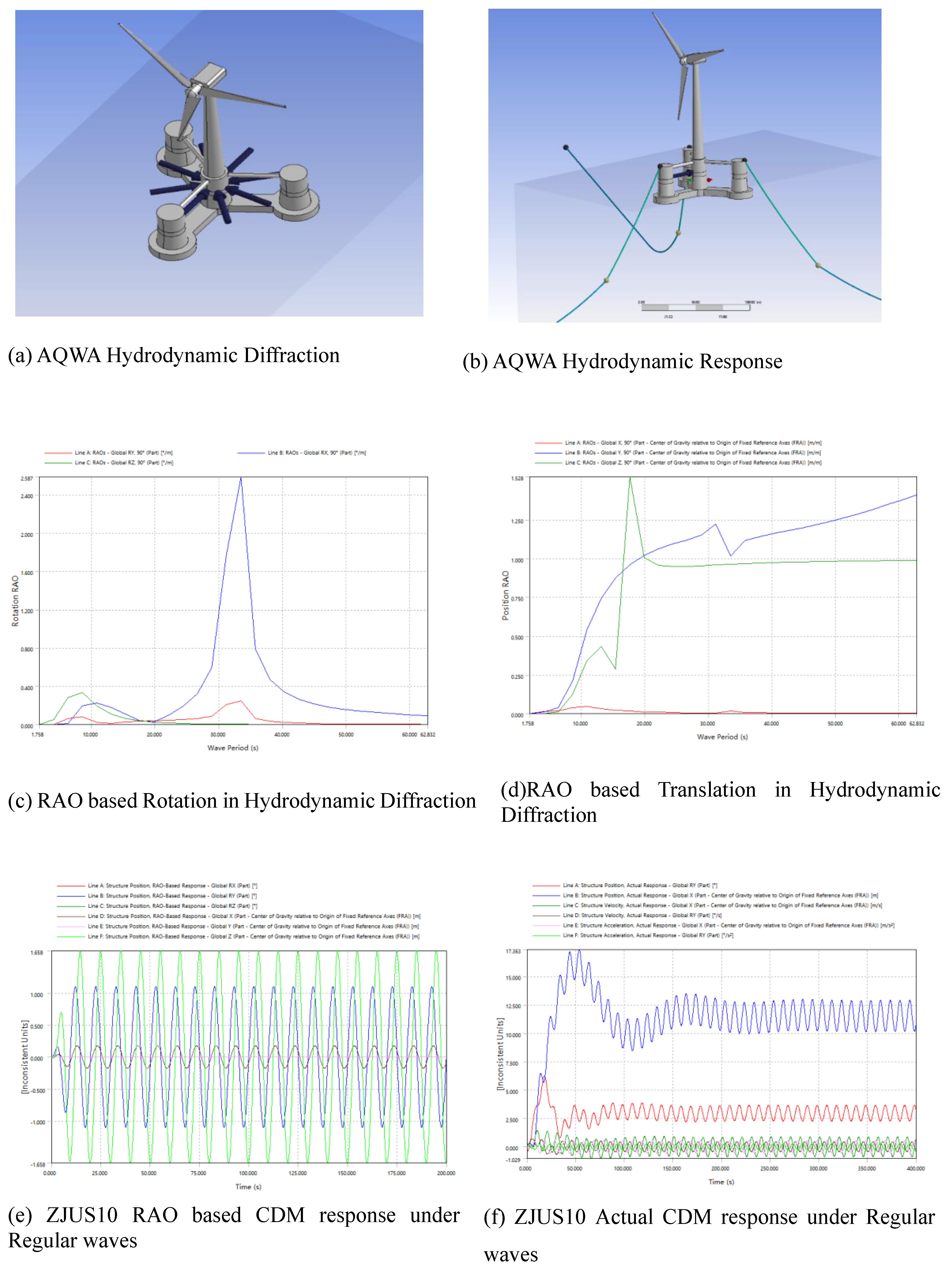
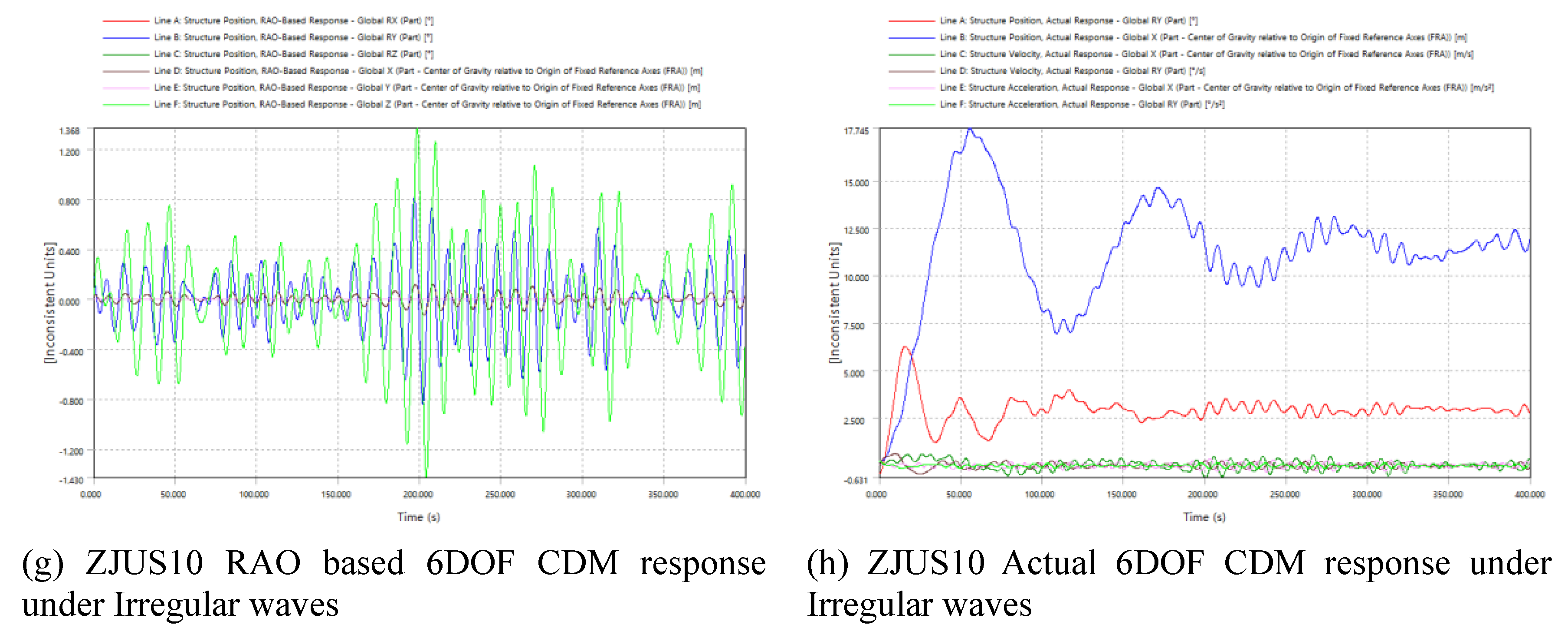
Figure 7.
ZJUS10 Stress analysis.
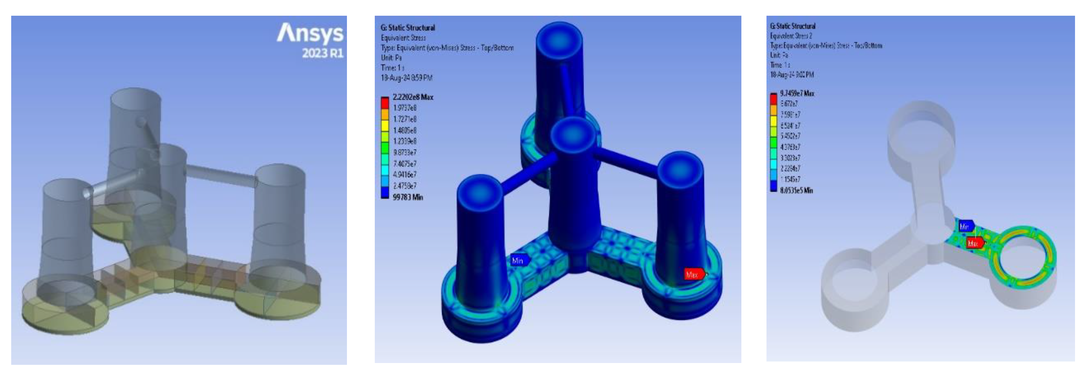
Figure 8.
Sensitivity Analysis of ZJUS10.
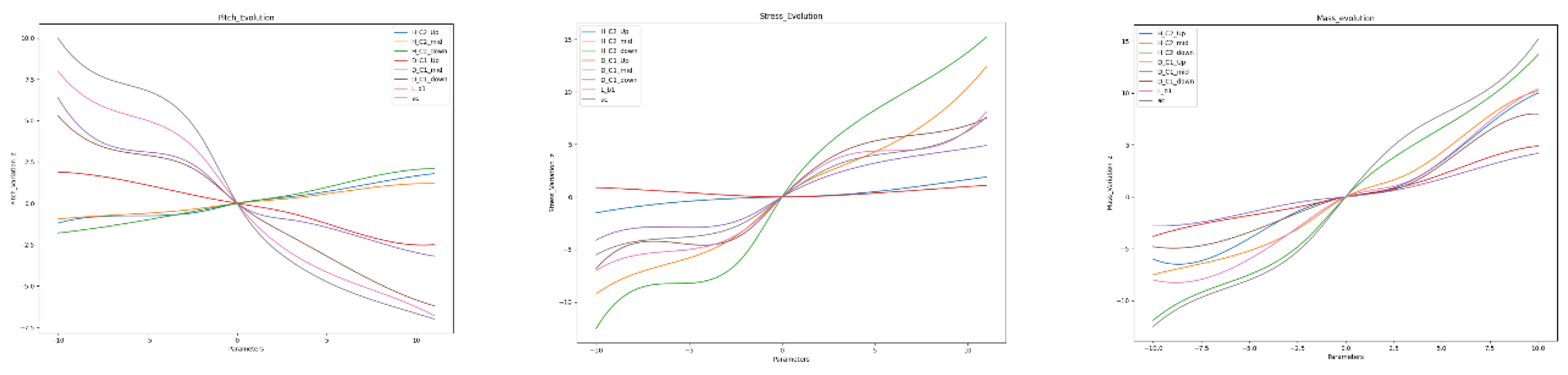
Figure 9.
Manufactured platform and experiment setup.
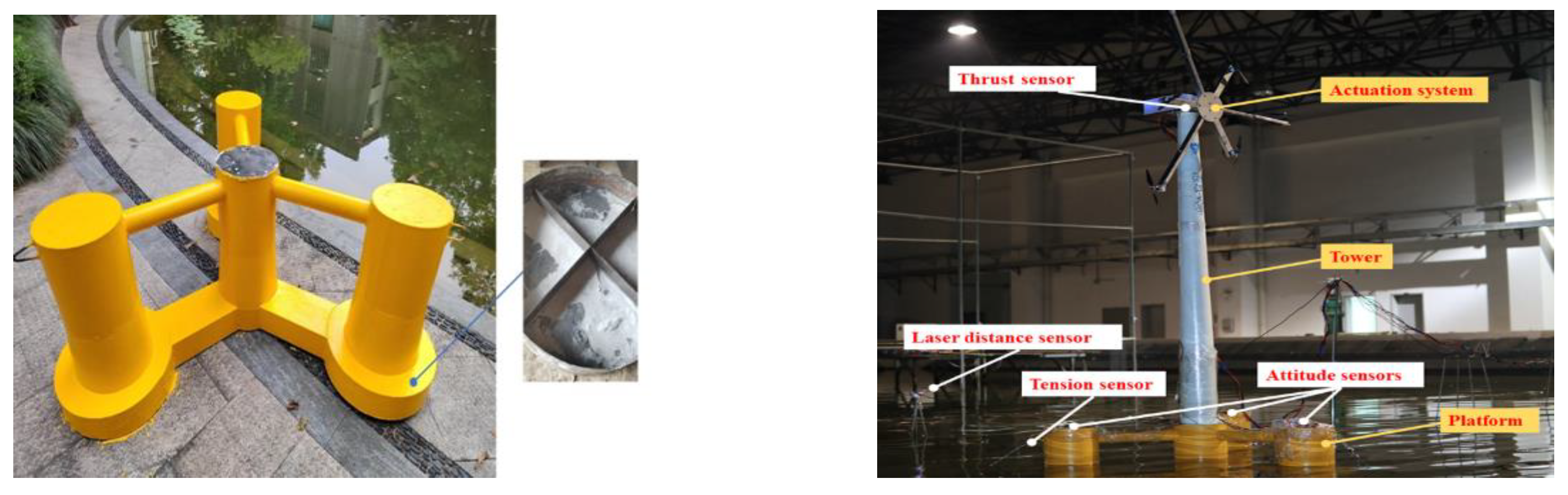
Figure 13.
3D Pareto Fronts generated of PSO, SA and ACO.
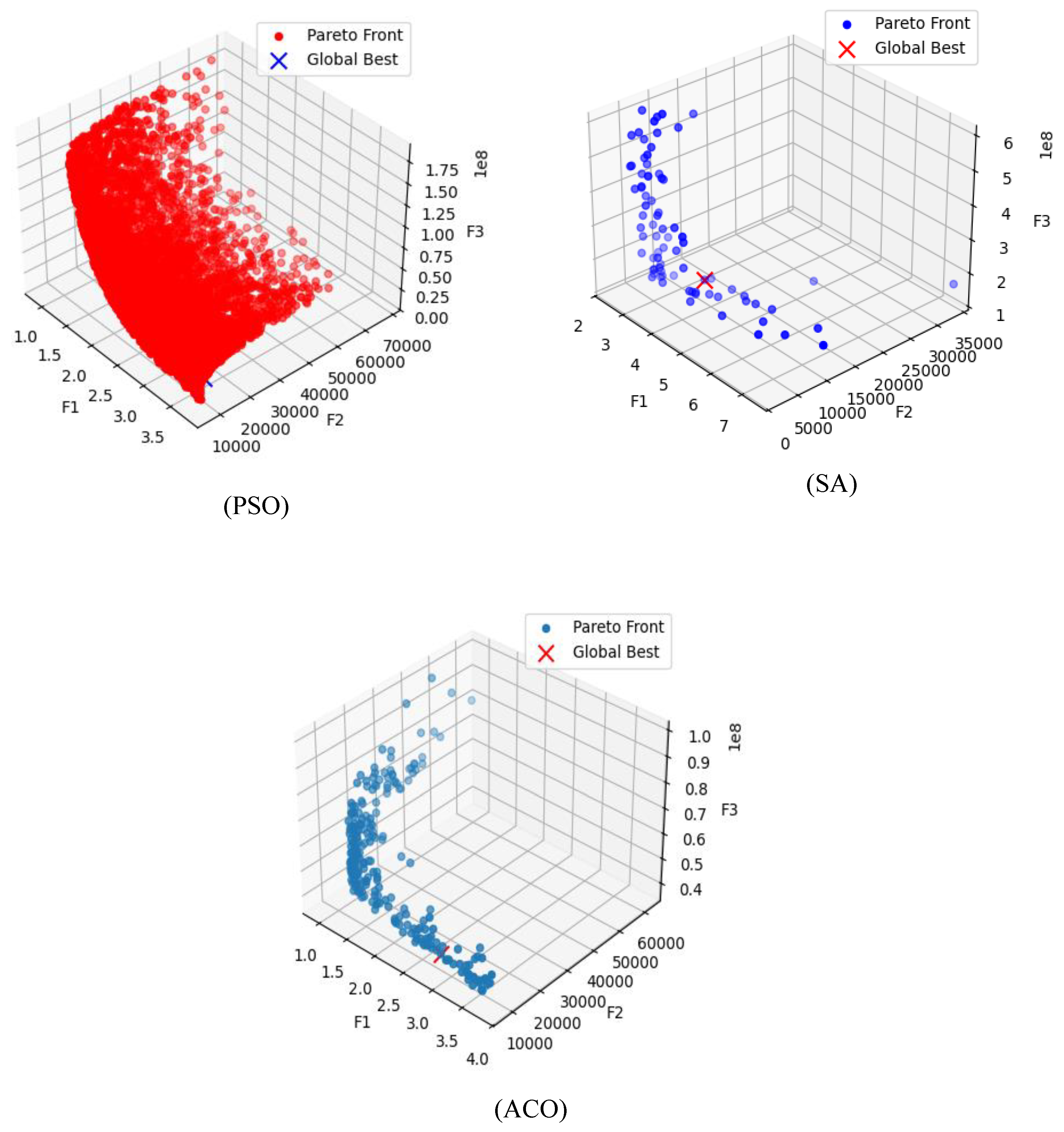
Figure 14.
Optimized models built on PyMAPDL.
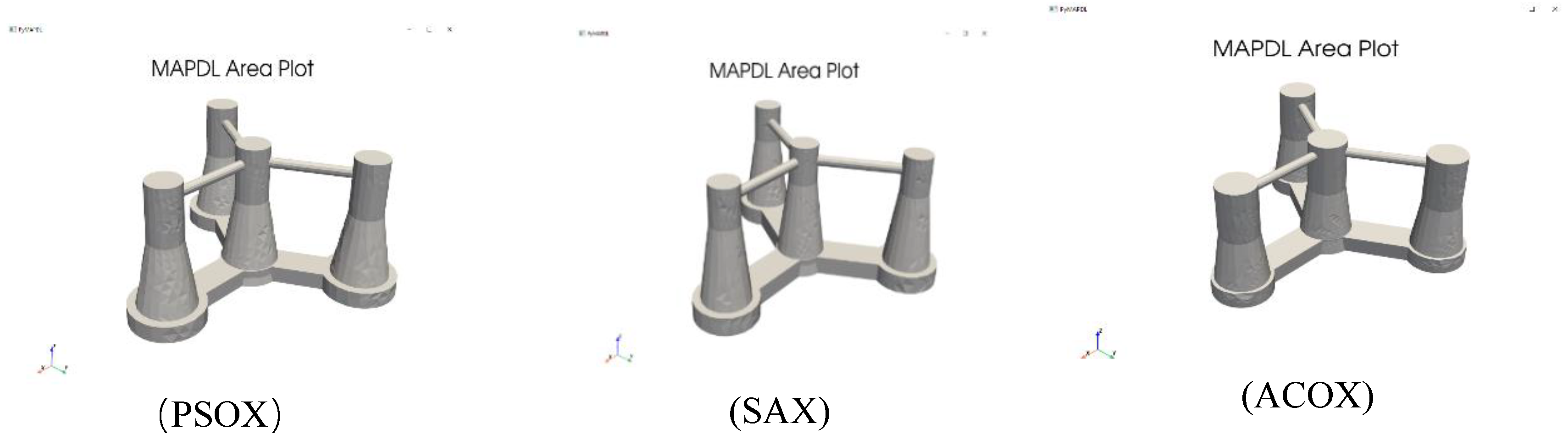
Figure 16.
Von Mises Stress results from PyMapdl.
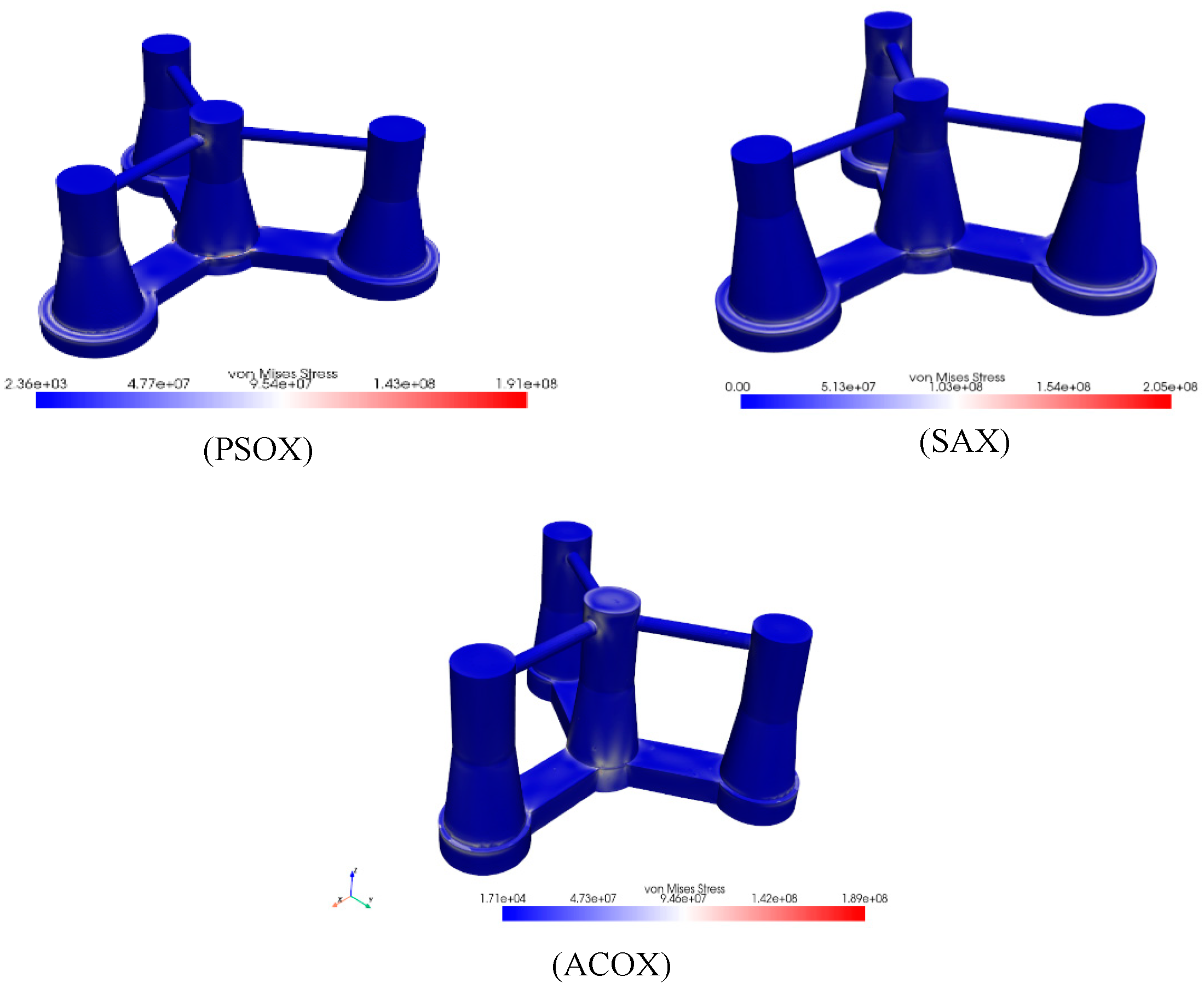
Table 2.
Coordinates of the 10MW wind turbine.
| Parameter | Value |
| Rated power | 10 MW |
| Rated wind speed | 11.4 m/s |
| Rated rotation speed | 9.6 RPM |
| Rated blade tip speed | 90 m/s |
| Rotor, hub diameter | 178.3 m,5.6 m |
| Hub height | 119 m |
| Shaft tilt, pre-cone | 5°, 2.5° |
Table 4.
ZJUS10 Parameters to optimize.
| Parameters to optimize | Initial Values | Bound Constraints |
| ac | 69 | [ , β ]; [ , λ ] |
| D_c1_up | 9.1 | [ , β ]; [ , λ ] |
| D_c1_mid | 16 | [ , β ]; [ , λ ] |
| D_c1_down | 19.3 | [ , β ]; [ , λ ] |
| D_b1_down | 10 | [ , β ]; [ , λ ] |
| H_c1_up | 16 | [ , β ]; [ , λ ] |
| H_c1_mid | 12 | [ , β ]; [ , λ ] |
| H_c1_down | 6 | [ , β ]; [ , λ ] |
| D_b1_up | 3 | [ , β ]; [ , λ ] |
Table 5.
Optimized Coordinates.
| Parameters | PSOX | SAX | ACOX |
| ac | 71.2 | 74.7 | 70.4 |
| D_c1_up | 9.1 | 22 | 11.8 |
| D_c1_mid | 16 | 17 | 17.9 |
| D_c1_down | 19.3 | 25 | 19.9 |
| D_b1_down | 9.6 | 8 | 11.3 |
| H_c1_up | 11.2 | 6 | 17.1 |
| H_c1_mid | 25.2 | 14 | 15.9 |
| H_c1_down | 5.4 | 2 | 5.4 |
| D_b1_up | 2.9 | 3 | 3.2 |
Table 6.
Triple Optimal Values.
| Objectives | ZJUS10 | PSOX | SAX | ACOX |
| Mass + ballast | 2.4e7 | 2.11e7 | 1.92e7 | 1.94e7 |
| Pitch (static, dynamic) | 3.9, 5.6 | 3.3, 3.1 | 2.4, 4.7 | 1.9, 2.3 |
| Max Stress | 2.2e8 | 1.91e8 | 1.99e8 | 1.87e8 |
Disclaimer/Publisher’s Note: The statements, opinions and data contained in all publications are solely those of the individual author(s) and contributor(s) and not of MDPI and/or the editor(s). MDPI and/or the editor(s) disclaim responsibility for any injury to people or property resulting from any ideas, methods, instructions or products referred to in the content. |
© 2024 by the authors. Licensee MDPI, Basel, Switzerland. This article is an open access article distributed under the terms and conditions of the Creative Commons Attribution (CC BY) license (http://creativecommons.org/licenses/by/4.0/).
Copyright: This open access article is published under a Creative Commons CC BY 4.0 license, which permit the free download, distribution, and reuse, provided that the author and preprint are cited in any reuse.


