
Submitted:
26 October 2024
Posted:
28 October 2024
You are already at the latest version
Abstract
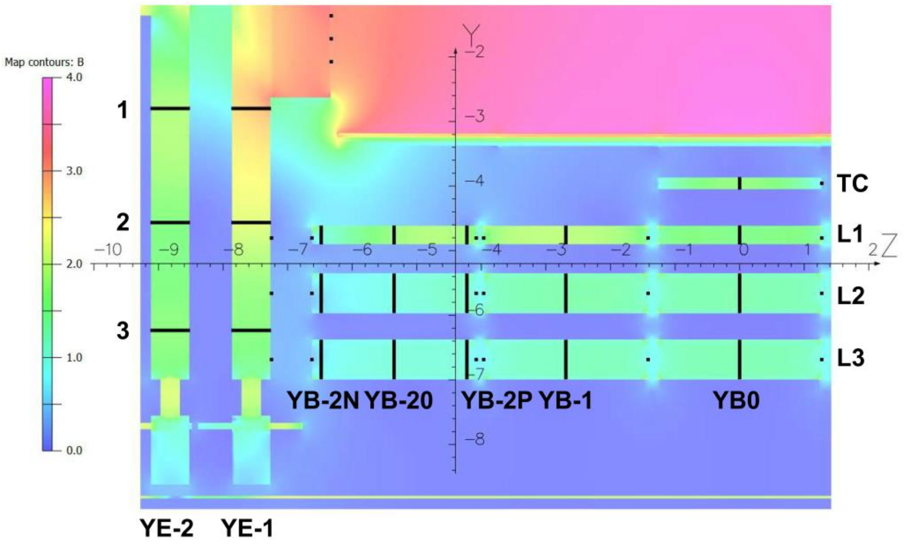
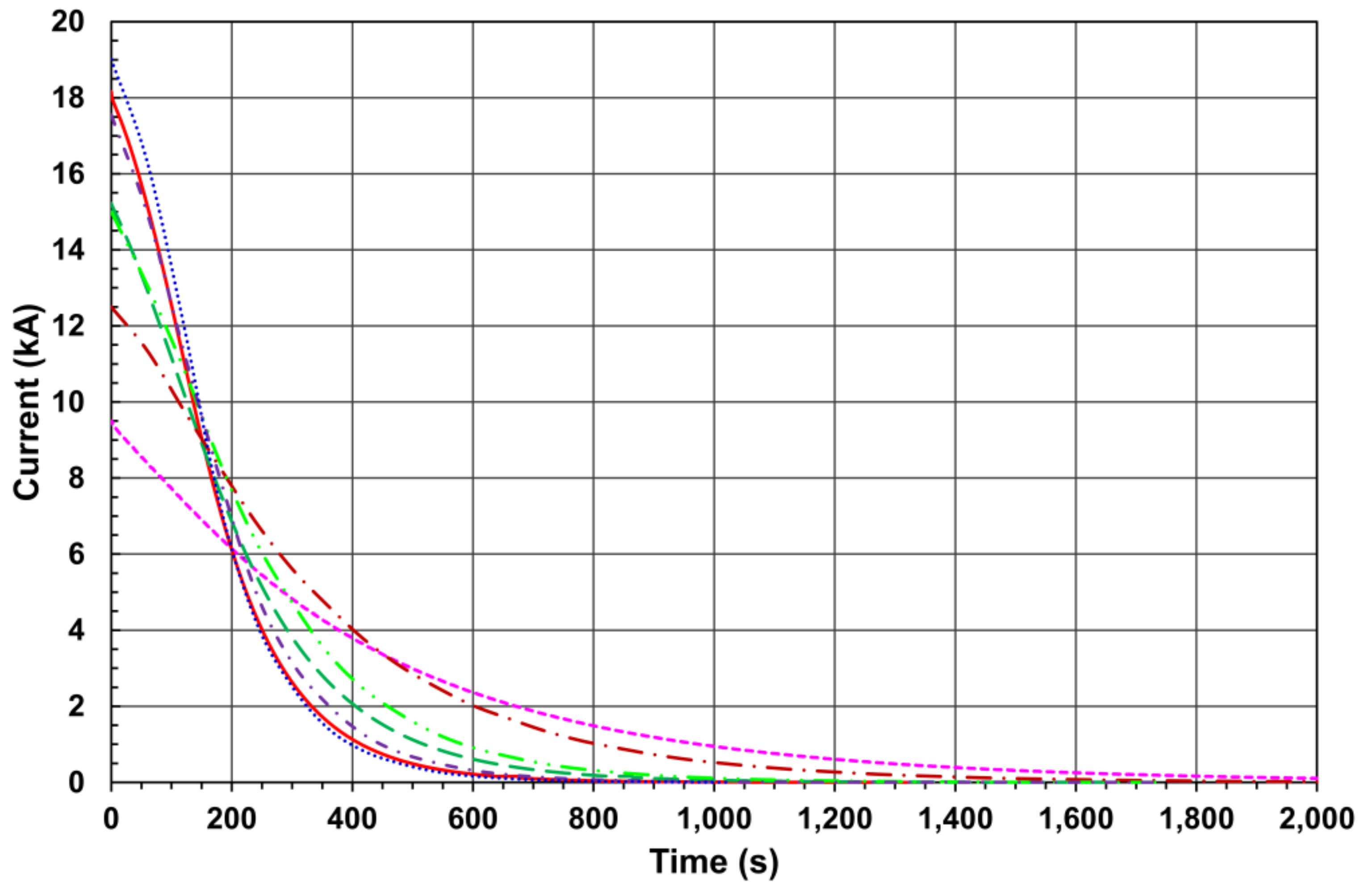
The general-purpose Compact Muon Solenoid (CMS) detector at the Large Hadron Collider (LHC) at CERN studies a production of new particles in the proton-proton collisions at the LHC center of mass energy 13.6 TeV. The detector includes the magnet based on the 6 m diameter superconducting solenoid coil operating with the current of 18.164 kA. This current creates a central magnetic flux density of 3.8 T that allows to measure momenta of the produced in collisions charged particles with tracking and muon subdetectors at a high precision. The CMS magnet contains a 10,000 ton flux-return yoke made of construction steel that bends muons in steel blocks magnetized with the solenoid returned magnetic flux. To reconstruct the muon trajectories, and thus, to measure the muon momenta, the drift tube and cathode strip chambers are located between the layers of the steel blocks and serve for this purpose. To describe the distribution of the magnetic flux in the magnet yoke layers, a three-dimensional computer model of the CMS magnet is used. To prove the calculations, the special measurements are performed with the flux loops wound in 22 cross-sections of the flux-return yoke blocks. The measured voltages induced in the flux loops during the CMS magnet ramp ups and downs, as well as during the superconducting coil fast discharges with the 190 s time constant, are integrated over time to obtain the initial magnetic flux densities in the flux loop cross-sections. The measurements obtained during the seven standard ramp downs of the magnet have been analyzed in 2018. From that time three fast discharges are occurred during the standard ramp downs of the magnet. This allows to single out the contributions of the eddy currents, induced in steel, to the flux loop voltages registered during the fast discharges of the coil. Accounting for these contributions to the flux loop measurements during manually triggered fast discharges in 2006 allows to perform the validation of the CMS magnet computer model with a better precision. The technique of the flux loop measurements, and the obtained results are presented and discussed.
Keywords:
1. Introduction
2. Materials and Methods
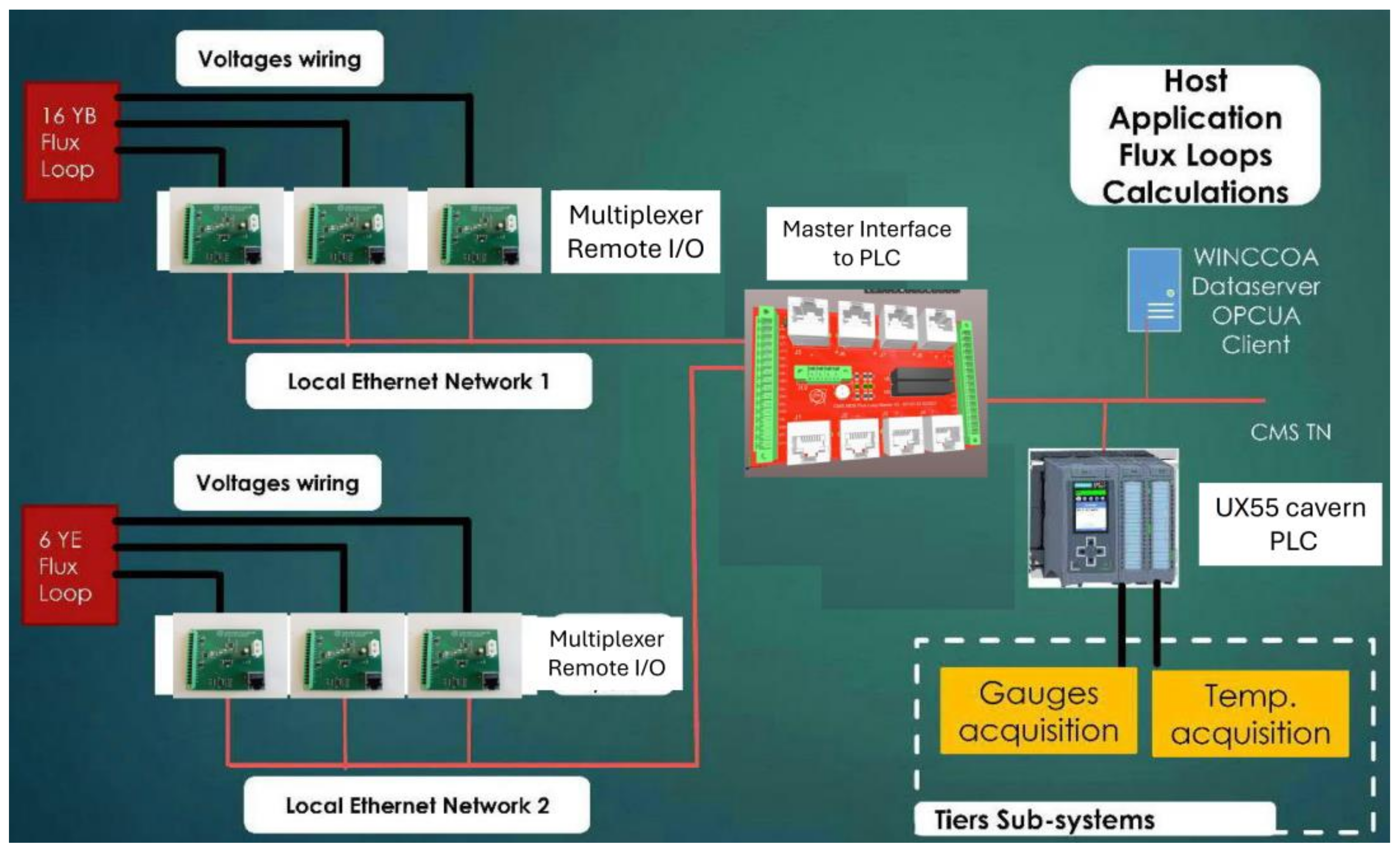
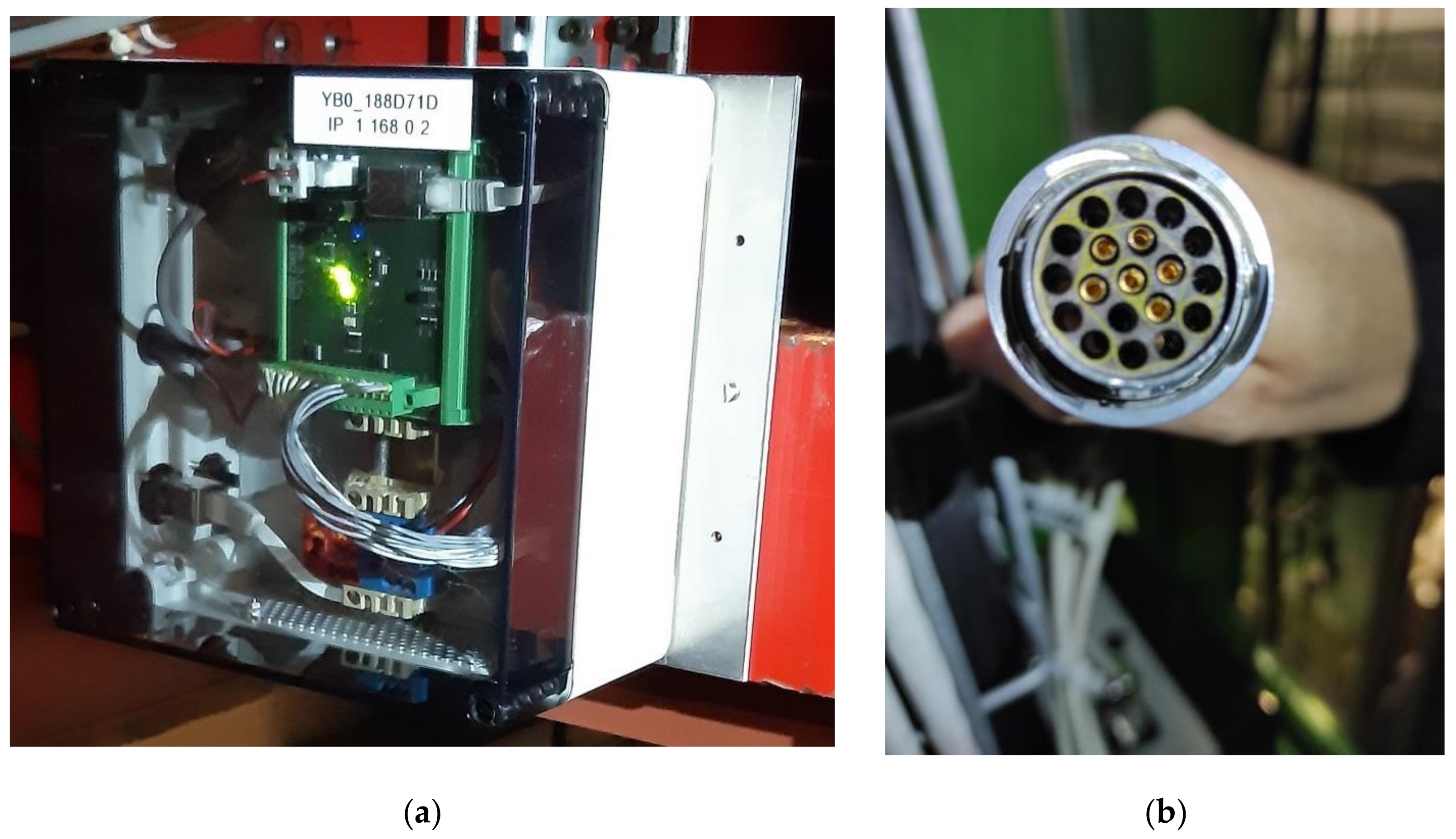
2.1. Description of the Flux Loop Measuring System
2.2. Estimation of the Eddy Current Contribution into the Induced Voltages
3. Results
4. Discussion
5. Conclusions
Author Contributions
Funding
Data Availability Statement
Acknowledgments
Conflicts of Interest
References
- CMS Collaboration. The CMS experiment at the CERN LHC. J. Instrum. 2008, 3, S08004. [Google Scholar] [CrossRef]
- Evans, L.; Bryant, P. LHC Machine. J. Instrum. 2008, 3, S08001. [Google Scholar] [CrossRef]
- Hervé, A. Constructing a 4-Tesla large thin solenoid at the limit of what can be safely operated. Mod. Phys. Lett. A 2010, 25, 1647–1666. [Google Scholar] [CrossRef]
- CMS Collaboration. Performance of the CMS drift tube chambers with cosmic rays. J. Instrum. 2010, 5, T03015. [Google Scholar] [CrossRef]
- CMS Collaboration. Performance of the CMS cathode strip chambers with cosmic rays. J. Instrum. 2010, 5, T03018. [Google Scholar] [CrossRef]
- Klyukhin, V.; Ball, A.; Bergsma, F.; Campi, D.; Curé, B.; Gaddi, A.; Gerwig, H.; Hervé, A.; Korienek, J.; Linde, F.; et al. Measurement of the CMS Magnetic Field. IEEE Trans. Appl. Supercond. 2008, 18, 395–398. [Google Scholar] [CrossRef]
- Klyukhin, V.; Ball, A.; Bergsma, F.; Boterenbrood, H.; Curé, B.; Dattola, D.; Gaddi, A.; Gerwig, H.; Hervé, A.; Loveless, R.; et al. The CMS Magnetic Field Measuring and Monitoring Systems. Symmetry 2022, 14, 169. [Google Scholar] [CrossRef]
- Klyukhin, V. Design and Description of the CMS Magnetic System Model. Symmetry 2021, 13, 1052. [Google Scholar] [CrossRef]
- TOSCA/OPERA-3d 18R2 Reference Manual; Cobham CTS Ltd.: Kidlington, UK, 2018; pp. 1–916.
- Simkin, J.; Trowbridge, C. Three-dimensional nonlinear electromagnetic field computations, using scalar potentials. In IEE Proceedings B Electric Power Applications; Institution of Engineering and Technology (IET): London, UK, 1980; 127, 368–374. [CrossRef]
- Klyukhin, V.I.; Amapane, N.; Andreev, V.; Ball, A.; Curé, B.; Hervé, A.; Gaddi, A.; Gerwig, H.; Karimaki, V.; Loveless, R.; et al. The CMS Magnetic Field Map Performance. IEEE Trans. Appl. Supercond. 2010, 20, 152–155. [Google Scholar] [CrossRef]
- Amapane, N.; Klyukhin, V. Development of the CMS Magnetic Field Map. Symmetry 2023, 15, 1030. [Google Scholar] [CrossRef]
- Campi, D.; Curé, B.; Gaddi, A.; Gerwig, H.; Hervé, A.; Klyukhin, V.; Maire, G.; Perinic, G.; Bredy, P.; Fazilleau, P.; et al. Commissioning of the CMS Magnet. IEEE Trans. Appl. Supercond. 2007, 17, 1185–1190. [Google Scholar] [CrossRef]
- Klyukhin, V.I.; Amapane, N.; Ball, A.; Curé, B.; Gaddi, A.; Gerwig, H.; Mulders, M.; Hervé, A.; Loveless, R. Measuring the Magnetic Flux Density in the CMS Steel Yoke. J. Supercond. Nov. Magn. 2012, 26, 1307–1311. [Google Scholar] [CrossRef]
- Klyukhin, V.; Campi, D.; Curé, B.; Gaddi, A.; Gerwig, H.; Grillet, J.P.; Hervé, A.; Loveless, R.; Smith, R.P. Developing the Technique of Measurements of Magnetic Field in the CMS Steel Yoke Elements with Flux-loops and Hall Probes. IEEE Trans. Nucl. Sci. 2004, 51, 2187–2192. [Google Scholar] [CrossRef]
- Klyukhin, V., Curé, B., Amapane, N., Ball, A., Gaddi, A., Gerwig, H., Hervé, A., Loveless, R., Mulders, M. Using the Standard Linear Ramps of the CMS Superconducting Magnet for Measuring the Magnetic Flux Density in the Steel Flux-Return Yoke. IEEE Trans. Magn. 2019, 55, 8300504. [CrossRef]
- Siemens AG Digital Industries. Functional manual SIMATIC S7-1500; A5E03735815-AL; SIEMENS: Nurnberg, Germany, 2023. Available online: https://support.industry.siemens.com/cs/attachments/59192925/s71500_communication_function_manual_en-US_en-US.pdf (accessed on 25 July 2024).
- Measurement Computing Corporation, Norton, MA, USA.
- Digi International Inc., Minnetonka, MN, USA.
- 3Com Corporation, Marlborough, MA, USA.
- Klyukhin, V.I., Amapane, N., Ball, A., Curé, B., Gaddi, A., Gerwig, H., Mulders, M., Hervé, A., Loveless, R. Flux Loop Measurements of the Magnetic Flux Density in the CMS Magnet Yoke. J. Supercond. Nov. Magn. 2017, 30, 2977–2980. [CrossRef]
- Klyukhin, V.; on behalf of the CMS Collaboration. Influence of the high granularity calorimeter stainless steel absorbers onto the Compact Muon Solenoid inner magnetic field. SN Appl. Sci. 2022, 4, 235. [CrossRef]

| Current (kA) | L1&TC | L2 | L3 | EC−1 | EC−2/1 | Barrel | Endcap | Yoke |
|---|---|---|---|---|---|---|---|---|
| 9.5 | 9.96 ± 5.17 | 5.53 ± 2.43 | 2.67 ± 0.47 | 5.88 ± 0.33 | 7.50 | 6.30 ± 4.53 | 6.28 ± 0.85 | 6.29 ± 4.04 |
| 12.5 | 8.85 ± 4.73 | 4.74 ± 2.02 | 1.66 ± 1.16 | 5.68 ± 0.40 | 5.05 | 5.32 ± 4.29 | 5.52 ± 0.45 | 5.36 ± 3.82 |
| 15 | 8.07 ± 4.74 | 4.37 ± 2.00 | 1.83 ± 0.94 | 5.30 ± 0.73 | 3.77 | 4.97 ± 4.01 | 4.92 ± 0.97 | 4.96 ± 3.58 |
| 15.221 | 6.68 ± 6.81 | 4.38 ± 2.02 | 1.81 ± 0.96 | 5.25 ± 0.75 | 3.70 | 4.44 ± 4.60 | 4.86 ± 0.99 | 4.53 ± 4.11 |
| 17.55 | 7.43 ± 4.83 | 4.48 ± 2.04 | 1.84 ± 0.96 | 4.94 ± 0.46 | 3.19 | 4.76 ± 3.85 | 4.51 ± 0.95 | 4.71 ± 3.45 |
| 18.164 | 7.98 ± 5.09 | 4.86 ± 2.26 | 1.79 ± 1.56 | 5.01 ± 0.25 | 3.16 | 5.27 ± 4.25 | 4.39 ± 1.08 | 5.44 ± 3.80 |
| 19.14 | 7.10 ± 4.89 | 4.69 ± 2.08 | 1.93 ± 0.93 | 4.63 ± 0.15 | 3.20 | 4.73 ± 3.77 | 4.28 ± 0.73 | 4.64 ± 3.37 |
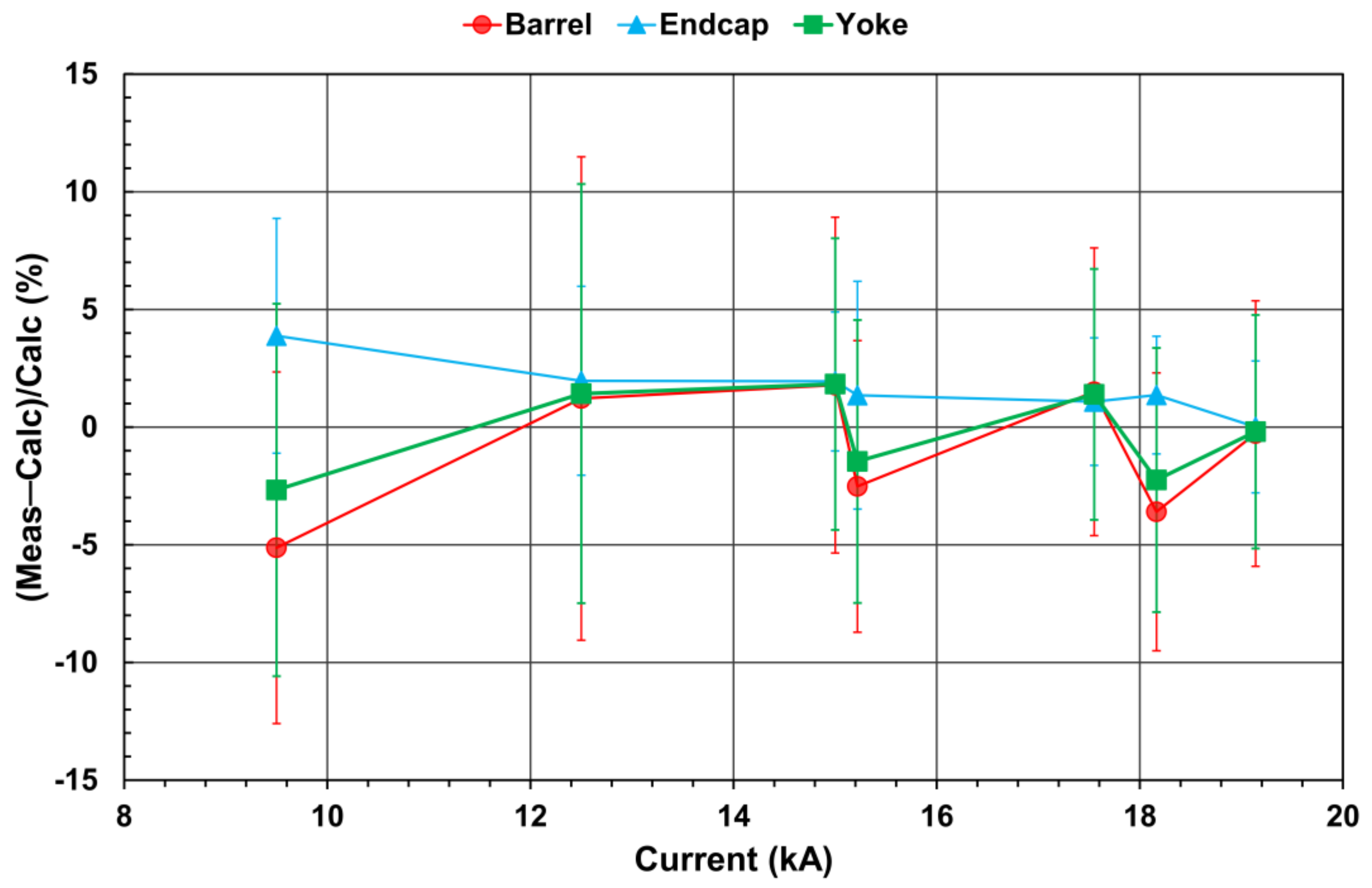
| Current (kA) | L1&TC | L2 | L3 | EC−1 | EC−2 | Barrel | Endcap | Yoke |
|---|---|---|---|---|---|---|---|---|
| 9.5 (new) | −3.60 ± 4.91 | −4.71 ± 7.74 | −7.39 ± 10.45 | 2.77 ± 3.38 | 4.98 ± 6.87 | −5.13 ± 7.47 | 3.88 ± 4.99 | −2.67 ± 7.92 |
| 12.5 (old) | −0.76 ± 10.15 | 7.65 ± 8.51 | −2.85 ± 10.79 | 0.69 ± 5.51 | 3.24 ± 2.22 | 1.22 ± 10.27 | 1.97 ± 4.01 | 1.42 ± 8.91 |
| 15 (old) | 2.30 ± 2.77 | 5.39 ± 7.27 | −2.44 ± 9.45 | 1.59 ± 2.37 | 2.29 ± 3.97 | 1.78 ± 7.13 | 1.94 ± 2.95 | 1.82 ± 6.20 |
| 15.221 (new) | 0.22 ± 1.30 | −2.61 ± 6.81 | −5.73 ± 8.44 | 1.09 ± 1.08 | 1.61 ± 7.57 | −2.52 ± 6.19 | 1.35 ± 4.84 | −1.46 ± 6.01 |
| 17.55 (old) | 3.16 ± 2.37 | 3.48 ± 5.53 | −2.47 ± 8.58 | 1.03 ± 1.06 | 1.14 ± 4.15 | 1.50 ± 6.11 | 1.08 ± 2.71 | 1.39 ± 5.33 |
| 18.164 (new) | −0.39 ± 0.84 | −4.58 ± 6.01 | −6.48 ± 8.17 | 0.09 ± 0.23 | 2.62 ± 3.29 | −3.60 ± 5.91 | 1.36 ± 2.50 | −2.25 ± 5.62 |
| 19.14 (old) | 1.66 ± 1.99 | 0.78 ± 5.07 | −3.66 ± 8.21 | 0.14 ± 0.67 | −0.13 ± 4.37 | −0.27 ± 5.64 | 0.005 ± 2.80 | −0.20 ± 4.96 |
Disclaimer/Publisher’s Note: The statements, opinions and data contained in all publications are solely those of the individual author(s) and contributor(s) and not of MDPI and/or the editor(s). MDPI and/or the editor(s) disclaim responsibility for any injury to people or property resulting from any ideas, methods, instructions or products referred to in the content. |
© 2024 by the authors. Licensee MDPI, Basel, Switzerland. This article is an open access article distributed under the terms and conditions of the Creative Commons Attribution (CC BY) license (http://creativecommons.org/licenses/by/4.0/).


