
Submitted:
25 October 2024
Posted:
29 October 2024
You are already at the latest version
Abstract
A recently developed differential geometric representation of redundant serial robot kinematics is employed to create an extended operational space dynamics and control formulation that explicitly accounts for redundant robot degrees of freedom. This formulation corrects deficiencies in kinematics and dynamics of redundant serial robots that have relied for over half a century on error prone generalized inverse velocity-based kinematics for redundancy resolution. New ordinary differential equations of robot operational space dynamics are obtained, without the need for ad-hoc derivation, in terms of task coordinates and self-motion coordinates that represent robot redundancy. A new extended operational space control approach is presented that exploits ordinary differential equations of motion in term of task and self-motion coordinates. This enables enforcement of desired output trajectories, in tandem with direct enforcement of self-motion dependent operational space trajectories that are subject to obstacle avoidance and performance constraints. Four examples are presented with a one degree of redundancy robot that demonstrate validity and superior performance of the new formulation, relative to traditional task space methods used for redundant serial robot control. Finally, an example with eight degrees of redundancy is presented that further illustrates superior performance of the new formulation.
Keywords:
Redundant Serial Robots
; Robot Dynamics
; Robot Control
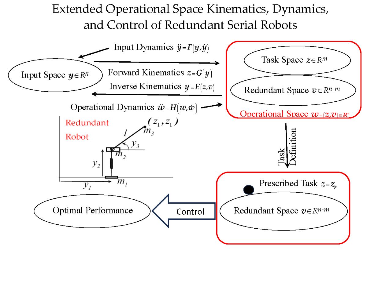
Introduction
1.Redundant Manipulator Kinematics and Control
The excess in number of control inputs over the number of functional outputs that characterize performance of kinematically redundant serial robots provides an opportunity to achieve a desired output (or task) trajectory, while simultaneously optimizing selected measures of robot performance [1]. With this opportunity, however, come challenges in creating a mathematical representation of robot kinematics and dynamics that quantitively represents robot redundant degrees of freedom, including an infinite number of inputs that yield a given output. The generalized inverse velocity space kinematics model of redundant robots originally presented by Whitney [2] has been shown to suffer serious deficiencies that have limited its ability to exploit benefits of redundant robot control. A method has recently been presented that analytically and computationally characterizes nonlinear set-valued robot inverse kinematics at the position and orientation level [3], correcting deficiencies due to the generalized inverse velocity approach. This formulation yields an extended operational space and ordinary differential equations (ODE) of dynamics that explicitly represent the versatility provided by robot redundancy and are ideally suited for robot control.
1.The Traditional Task Space Formulation
A substantial redundant robotics literature has evolved based on a task space formulation introduced by Khatib [4], using robot models based on task (or output) coordinates. To date, models of redundant serial robots in the traditional task space formulation have been based on mass-corrected generalized inverse velocity space kinematics that suffer kinematic and kinetic error. A theoretical, computational, and experimental analysis of eight controllers based on velocity, acceleration, and force redundancy resolution [5], compared with the traditional task space formulation [4], showed that the latter suffers significant inaccuracies.
To compensate for errors associated with the traditional task space formulation, Park et. [6] proposed an extended operational velocity space that introduced self-motion velocities to complement task space velocities that are employed in the traditional formulation. While these additional terms yield a linear approximation of redundant robot degrees of freedom, the associated velocity space kinematics fail to define an accurate model of redundant robot dynamics.
A new redundant robot inverse kinematics formulation at the position and orientation level [3] is employed herein, using differential geometry for definition of a redundant serial robot extended operational space. This space is parameterized by operational coordinates that include self-motion coordinates that accurately account for redundant robot degrees-of-freedom. Extended operational space ODE of dynamics are derived that are equivalent to robot multibody dynamics ODE in input coordinates and explicitly account for redundant degrees of freedom. A new control approach is presented, using the extended operational space ODE for accurate tracking of a desired output trajectory, while enforcing obstacle avoidance and optimization of selected measures of robot performance. This approach corrects deficiencies identified in [5] that degrade performance of traditional task space control and approximation errors induced by the extended operational velocity space formulation [6].
1.Organization of the Paper and its Contributions
The kinematic structure of redundant serial robots is defined in Section 2 and deficiencies of generalized inverse velocity space kinematics are identified. Equations of robot kinematics in task and self-motion coordinates are presented in Section 3 using differential geometry, leading to a new extended operational space formulation that resolves deficiencies associated with generalized inverse velocity space kinematics. A new system of redundant robot operational space ODE of dynamics is presented in Section 4 that explicitly accounts for robot redundancy and is equivalent to the equations of robot multibody dynamics in input coordinates. A new control approach based on the extended operational space ODE is presented and illustrated with four applications of a one degree of redundancy serial robot in Section 5 and a higher dimensional example in Section Finally, conclusions and recommendations for future research are presented in Section 7.
The primary contributions of the paper are as follows:
- An explicit set-valued inverse kinematic mapping is derived for input coordinates as functions of task and self -motion coordinates.
- Extended operational coordinates are shown to be equivalent to input coordinates in parameterizing robot configuration space.
- ODE of robot dynamics are derived with extended operational coordinates as state variables.
- Robot control laws are defined and implemented using extended operational coordinates and operational space ODE.
- Four control examples are treated using a redundant planar robot with one degree of redundancy, demonstrating superior performance of the extended operational space formulation relative to the traditional task space approach.
- A control example is treated for a robot with eight degrees of redundancy, further demonstrating superiority of the extended operational space appproach.
Redundant Serial Robot Kinematics
A redundant serial robot is comprised of a chain of bodies that are connected by single degree of freedom joints. Joint relative input coordinates between bodies in the chain define the position and orientation of outboard bodies, relative to their inboard counterparts. The terminal body in the chain is the end effector, whose output coordinates characterize its working capability, defined as twice continuously differentiable functions of input coordinates , n > m, in the forward kinematic mapping
where input coordinates are independent generalized coordinates that define the configuration of the underlying mechanism [7]. Here, refers to k-dimensional Euclidean space with elements in the form of column vectors and superscript T denotes matrix transpose. Bold characters denote vectors and matrices.
2.Velocity Space Kinematics
For over half a century, kinematics of redundant serial robots has been modeled in velocity space, yielding fundamental deficiencies in representation of both kinematic and dynamic performance. In 1969, Whitney [2] made a significant contribution to resolved motion rate control of serial robots, using the Moore-Penrose generalized inverse to obtain an approximate velocity space inverse kinematic mapping. Since of Eq. (1) is twice continuously differentiable, an apparent velocity differential equation is obtained by differentiating Eq. (1) with respect to time,
where the Jacobian matrix has full row rank for redundant serial robots with no inverse kinematic singularities [3]. The Moore-Penrose generalized inverse,
that satisfies , is applied to Eq. (2) to obtain an inverse velocity mapping,
where, with arbitrary, the second term on the right yields velocities in the null space of . This velocity space kinematics formulation, with minor variations, has been used to represent redundant serial robot kinematics for half a century [1].
2.Deficiencies in Redundant Robot Velocity Space Kinematics
The first deficiency in velocity space kinematics is that Eq. (2) is not an ODE. Written in the differential form 0, it is seen to be a Pfaffian differential equation [8] that behaves more like a partial differential equation than an ODE and is extremely difficult to solve. The second deficiency is that in Eq. (3) is generally not a total differential; i.e., Eq. (4) is generally nonholonomic and yields nonperiodic, or noncyclic, solutions for , even if is periodic [3,9,10,11]. The third, and most critical deficiency, is that the velocity space inverse kinematic mapping of Eq. (4) does not lead to valid ODE of robot dynamics. These deficiencies have been known for a quarter century [9,10,12,13], but they remain largely unresolved.
Early research on resolving deficiencies in the velocity space kinematics approach focused on physically-based concepts such as introducing artificial damping, using impedance control, and carrying out torque optimization [14,15,16]. More recent research has focused on using numerical methods such as adaptive extended Jacobians and null space projections [17,18]. These papers cite well over 100 additional papers that have sought to resolve the deficiencies noted above. Some progress has been reported, but deficiencies in the velocity space kinematics approach remain.
2.Traditional Task Space Dynamics of Redundant Serial Robots
The Moore-Penrose generalized inverse of Eq. (3) represents a purely kinematic approach to robot analysis, since it contains no inertial information. The traditional task space approach [4] was introduced to address kinetics by including inertia effects into definition of the generalized inverse matrix and projecting dynamics into task-space. In the non-redundant case n = m, when the Jacobian is nonsingular, any applied robot input space generalized force can be produced by a task space force acting at the task point; e.g., the end effector, along task coordinates. The applied generalized force is then obtained as , using the principle of virtual work [7,19]. In the case of redundant robots, a null space projection term , , is needed as a complement to the task term, in order to represent an arbitrary applied generalized force.
where is the symmetric positive definite mass matrix, is a vector of applied generalized forces that act on and between bodies in the robot chain, and is a vector of velocity coupling terms (sometimes called Coriolis forces). The term will be restricted here to gravitational force; i.e., . The left side of Eq. (5) represents the decomposition of input space generalized forces into task space and null space terms, . Multiplying Eq. (5) by , noting that , rearranging terms, and suppressing arguments,
A condition can now be imposed to assure that the term associated with the null space does not contribute to task space acceleration. This has been defined as dynamic consistency [13] and is expressed as
for all , where represents an arbitrary generalized inverse of that satisfies the identity. Straightforward matrix algebra yields the transpose of the dynamically consistent generalized inverse [13] of the Jacobian,
Defining the symmetric positive definite task space mass matrix , the task space centrifugal and Coriolis force vector , and the task space gravity force vector [13], Eq (7) can be formally expressed as the task space equation of motion [4],
It is important to note that Eq. (9) does not constitute a system of ODE in z, since its terms are dependent on robot input coordinates y. It is shown in Section 3 that y cannot be written as an explicit function of z. The task coordinates and their derivatives, therefore, do not constitute state variables in this system of equations. Since are state variables for the robot, task coordinates must be augmented by additional coordinates to create a valid system of operational space generalized coordinates that serve as state variables. The traditional task space is thus not a state space for the redundant robot.
The Extended Operational Space
To extend the velocity space formulation of Section 2.1 to robot configuration (position and orientation) space, it is required that a set-valued inverse kinematic mapping be constructed; i.e., a solution of Eq. (1) be found with an arbitrary vector of coordinates that define robot redundancy. Such a mapping has been presented in [3] for redundant serial robots, using differential geometry, and is summarized in this section. It is used in Section 4 to obtain a new system of extended operational space ODE of redundant robot dynamics.
3.Inverse Configuration Kinematics
An input-output pair defines a robot configuration. The robot configuration space is defined as 0}. It should be noted that configuration space in the robotics literature is often defined as the space of input (joint) coordinates. The robot configuration space defined herein is a subset of the product of input and output spaces [20,21] that satisfies Eq. (1). It thus embodies the topology of the robot, not just its input space. More specifically, X is the graph of Eq. (1) that is a differentiable manifold if is smooth and has full rank, with a single chart on X [21]. This is effectively a forward kinematic differentiable manifold, parameterized by .
To avoid inverse kinematic singular behavior that occurs at input coordinates for which the Jacobian matrix of is rank deficient [3], the regular robot configuration space is defined as . The entire regular robot configuration space cannot, in general, be characterized by a single continuously differentiable inverse kinematic mapping. The only practical global inverse kinematic mapping is based on concepts of differential geometry [21] that employ local kinematic representations on open sets , whose union is the regular robot configuration space; i.e., . In , is a base point about which an inverse kinematic mapping is constructed over .
For a given j and base point , define the matrix and an matrix such that
where is computed as a matrix whose columns form an orthonormal basis for the null space of ; e.g., in MATLAB, using singular value decomposition [22]. The matrices are defined to be constant on . Note from the second of Eqs. (10) that 0 and 0. Since has full rank, so do and . Further, since 0, the columns of and are mutually orthogonal. The n combined linearly independent columns of (m columns) and ( columns) therefore span . Using and of Eq. (10), any solution y of Eq. (1) in a neighborhood of can be written as
where are values of v and u associated with on a trajectory that first enters. They are introduced to assure continuity of y as a function of v and z in Eq. (11). In , 0 and 0. At , Eq. (11) implies .
To see that there is a unique solution of Eq. (1) with y of Eq. (11); i.e., of
for u as a function of z and v in a neighborhood of and , the derivative of the left side of Eq. (12) with respect to u, evaluated at , is , which is nonsingular. The implicit function theorem [23] implies existence of a unique, twice continuously differentiable solution of Eq. (12) in a neighborhood of . From Eq. (11),
This is the desired set-valued inverse kinematic mapping on , in which coordinates quantitatively define robot redundancy. Note that, in contrast with Eq. (4) that is linear in the free velocity , Eq. (13) is nonlinear in and represents nonlinear characteristics of redundant serial robots that cannot be characterized by Eq. (4).
If are periodic of period on ; i.e., and , and if Eq. (13) holds throughout , then . Thus, of Eq. (13) is periodic of period in and the robot is cyclic on , or locally cyclic. For more detail regarding cyclicity, see [10,11]. There is no basis to expect that the traditional task space approach is cyclic.
A computationally efficient iterative method for evaluation of is presented in Section 3.In this computation, when the number of iterations required for convergence in numerical solution of Eq. (12) exceeds a specified tolerance, the associated configuration is designated , y, v, and u are designated , , and , a new neighborhood is entered, and the parameterization of Eq. (13) is redefined. As shown in [19] for dynamic system simulation, less than 0.1% of CPU time and no user interaction is required for this reparameterization. For more detail on the process of selecting configurations and reparameterization calculations, see [3,19].
For a given output , with arbitrary in a neighborhood of , Eq. (13) defines a set of input coordinates, , called the robot self-motion manifold in input space associated with output . Since is the solution of Eq. (12), 0, for all v in a neighborhood of , of Eq. (13) maps into the same ; i.e., . Elements of the vector are thus called self-motion coordinates. With arbitrary self-motion coordinates v in a neighborhood of , Eq. (13) defines redundant degrees of freedom of the robot that enable it to meet requirements that could not be met with a nonredundant robot. Self-motion coordinates v thus explicitly represent robot redundancy at the configuration level. This fundamental new result is in stark contrast with the velocity space kinematic representation presented in Sections 2.1 and 2.2.
It is important to note that the self-motion manifold is defined at the robot configuration level and is nonlinear in . Since robot configuration information is not defined in the generalized inverse velocity formulation of Section 2.1, the self-motion manifold and self-motion coordinates are not available for obstacle avoidance and other performance optimization functions in the velocity space formulation. In fact, the second term of Eq. (4) that defines a projection onto the null space of leads to linear analysis in the velocity setting that only approximates the nonlinear self-motion manifold.
3.The Robot Extended Operational Space
Defining extended operational coordinates , the robot extended operational space W is the subset of such that for all in a neighborhood of , where . Thus, the set-valued inverse kinematic mapping of Eq. (13) is a twice continuously differentiable mapping from subsets of W into the robot input space. The fundamentally new space of extended operational coordinates and Eq. (13) define inverse kinematic relations at the robot configuration level; i.e., between task space position and orientation coordinates of bodies that make up the robot mechanism, self-motion coordinates, and input coordinates between bodies in the chain that defines the serial robot. This is in stark contrast with robot velocity relations of Section 2.1 that suffer severe deficiencies presented in Section 2.As will be shown in Section 4, the extended operational space formulation enables derivation of ODE of robot dynamics that are equivalent to input space ODE and correct deficiencies of the traditional task space dynamics formulation discussed in Section 2.3.
3.The Robot Functional Configuration Space
Defining robot functional coordinates , the robot functional configuration space is defined as. Similar to the definition of the robot configuration space as the subset of the product of input and output spaces that satisfy Eq. (1), is defined as the subset of the product of input and extended operational spaces that satisfy Eq. (13).
From Eq. (11), . This and the kinematic mapping of Eq. (1) define a y-parameterization of , , for in a neighborhood of . Conversely, the kinematic mapping of Eq. (13) enables the -parameterization of on . This duality of input and extended operational coordinate parameterizations of provides the foundation for a fundamentally new analytical and numerical representation of redundant serial robot kinematics and dynamics. The robot functional configuration space can be parameterized by either or . It cannot, however, be parameterized by only output z. It is thus not possible to obtain ODE of robot dynamics in only z, as is attempted in the traditional operational task space setting of Section 2.3 [4].
While has many of the characteristics of a differentiable manifold, the foregoing has not shown it is a differentiable manifold [21]. This leaves open questions regarding its singularity free domains of robot functgionality for future reseaarch.
Kinematics and dynamics on must be carried out on individual sets , called charts that cover , and transitioned to adjacent charts as robot configurations progress along a trajectory in , as shown schematically in Fig. Piecewise analysis on charts is unavoidable since, in general, there is no globally valid extended operational coordinate parameterization of . This attribute of differential geometry that transforms local to global properties of sets and mappings is one of its greatest contributions. The unavoidable reality, however, is that one must adopt local operational space parameterizations, since no global parameterization generally exists.
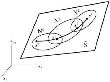
Figure Trajectory Along Charts in .
3.Velocity Kinematics on the Extended Operational Space
Differentiating the identity 0 on that is obtained by substituting of Eq. (13) into Eq. (1) with respect to t, suppressing index j for notational convenience, and recalling that are constant on, yields
The matrix is nonsingular and is a continuously differentiable matrix function of , so is nonsingular in a neighborhood of . The matrix
is therefore well defined and continuously differentiable in K. A computationally efficient iterative method for evaluation of is presented in Section 3.For readers who may be concerned with the cost of evaluating the inverse matrix in Eq. (15), note that its cost is no greater than that of evaluating in the generalized inverse of Eq. (3).
Substituting Eq. (15) into Eq. (14), . Differentiating Eq. (13) with respect to t, using this result and the chain rule of differentiation,
where . At , from Eq. (10), 0, so has full rank. Since is a continuous matrix function of y, has full rank in a neighborhood of . Matrix multiplication and use of Eq. (15) show that 0, so the columns of span the null space of in a neighborhood of .
Note that , so in Eq. (16) is a generalized inverse of and Eq. (16) is of the form of the ill-fated velocity space relation of Eq. (4), except that is comprised of independent self-motion velocities and appears in nonlinear form. The fundamental difference between Eqs. (4) and (16) is that the latter is the time derivative of Eq. (13); i.e., it is holonomic, and Eq. (4) is generally nonholonomic [10]; i.e., it is not the time derivative of any algebraic (holonomic) equation. This result is obtained without having to resort to use of the Frobenius theorem of differential geometry [9,10,21]. The inverse kinematic mapping of Eq. (13) thus resolves deficiencies in redundant robot velocity space kinematics summarized in Section 2.2 that have plagued redundant serial robot kinematics, dynamics, and control for half a century.
With extended operational coordinates that quantitatively represent robot output and redundancy, Eq. (16) may be written as
where . To see that the matrix is nonsingular, expand
This shows that is nonsingular and that
The explicit solution of Eq. (17) for is thus
3.Acceleration Kinematics on the Extended Operational Space
Differentiating Eq. (19) with respect to t, , where over hat denotes a variable that is held constant for the indicated partial differentiation. Thus,
where, with of Eq. (13) and of Eq. (17), .
3.6 Computation of
While vector and matrix functions for serial redundant robots are shown to exist and be differentiable functions of z, , and , their derivations do not show how to evaluate them. Since they are central to implementing kinematic position, velocity, and acceleration analysis, numerical methods for their evaluation are needed.
At , is numerically evaluated. For at time on a time grid, must satisfy Eq. (15), in the form 0. With an approximation of the solution and suppressing arguments , since they do not change in the iterative process for , a matrix version of Newton-Raphson iteration is, where (j) denotes iteration number. Since need not be inverted with great precision in the Newton-Raphson process [22] and , and . This yields the computationally efficient iterative algorithm that requires only matrix multiplication,
where Btol is error tolerance.
While cannot be analytically determined, it can be evaluated as accurately as desired using Newton-Raphson iteration to solve Eq. (12) for , with . The solution is and , i.e., the iterative algorithm
where utol is error tolerance. Since the Newton-Raphson method does not require an exact Jacobian [22], the matrix B is held constant throughout the process. This is an efficient computation, requiring only matrix multiplication.
ODE of Input and Extended Operational Space Dynamics
4.Input Space ODE of Dynamics
Since input is a vector of mechanism generalized coordinates, the d’Alembert variational equation of motion of a serial robot is [7,19]
which holds for all virtual displacements that satisfy the differential form of Eq. (1); i.e., . In Eq. (23), is a symmetric positive definite mass matrix, is a vector of applied generalized forces that act on and between bodies in the robot chain, is a vector of velocity coupling terms (sometimes called Coriolis forces), is a vector of input generalized forces, is a vector of generalized forces that act on the output frame due to its interaction with the environment, and shorthand notation is . Constraint reaction forces do not appear in this equation [7,19]. Substituting Eq. (1) and , into Eq. (23), 0, which holds for arbitrary . This yields the input space ODE of dynamics,
4.Extended Operational Space ODE of Dynamics
Substituting of Eq. (20), of Eq. (16), and of Eq. (13) into Eq. (24),
This is the extended operational space ODE of dynamics, which holds on each . Since are nonsingular, with initial conditions on w and , the extended operational space initial-value problem for the second order ODE of Eq. (25) is well posed; i.e., it has a unique solution that depends continuously on problem data [19].
For use in control system design, it is helpful to write Eq. (25) as an explicit system of differential equations in z and v, where and v represents robot redundancy. Substituting of Eq. (16) and of Eq. (20) into Eq. (23),
Since are arbitrary, this yields a coupled system of second order nonlinear extended operational space ODE in z and v that is ideally suited for control system design,
Nonlinear dependence of terms in Eq. (26) on z and v follows from the fact that the function of Eq. (13) and the function of Eq. (16) are nonlinear in z and v.
As motion of the system progresses over , reparameterizations in the extended operational space may be required in making the transition between charts, as depicted in Fig. 1 and outlined in Section 3.The requirement for reparameterization is an inconvenience that cannot be avoided, since global parameterizations of with operational coordinates do not generally exist. The computational cost of reparameterization is, however, minimal [19]. In the process of reparameterization, continuity of y,, z, and is enforced, leading to restart values
of v and , the latter obtained by multiplying Eq. (16) on the left by . As a result, is continuous but may be discontinuous at reparameterization times.
Since the functional operational space can be parameterized by either or and steps in the transformations from Eq. (24) to Eqs. (26) are reversible, the ODE of Eqs. (24) through (26) are equivalent; i.e., they have the same solutions. Without coordinates v , Eq. (26) in only output coordinates z could not be equivalent to robot ODE of multibody dynamics of Eq. (24). This shows that the ODE of Eq. (9) in the traditional task space formulation [4] cannot be equivalent to robot ODE of multibody dynamics.
4.A Single Degree of Redundancy Serial Robot Example
The redundant robot of Fig. 2 has three input coordinates and two output coordinates . Its kinematic equation is
with Jacobian . In addition to its analytical simplicity, this is an attractive example for analysis, since the Jacobian matrix is of full rank throughout robot configuration space. Any pathological behavior of the robot cannot, therefore, be attributed to a rank deficient Jacobian.
To obtain input space ODE of motion for the robot of Fig. 2, vectors that locate its three bodies, modeled as point masses in the plane, are , , and , where . Variations, or virtual displacements, of the mass locations are obtained by taking differentials of the , , , and . Accelerations of the masses are obtained by taking two derivatives of the , , , and . With these results, the d’Alembert variational equation of motion is [7,19],
where are input forces and torques and is the vector of external forces and torques that act on the end effector. Expanding products in Eq. (29), using , and , yields input ODE of motion of Eq. (24) with and . For the extended operational space ODE of Eq. (25), , , and . Since is nonsingular and is given by Eq. (18), suppressing arguments of functions for notational convenience, Eq. (25) may be written in the explicit ODE form
With initial conditions , and , associated , and output force , suppressing arguments, the input space ODE of Eq. (24) is
In the extended operational space ODE of Eq. (30), initial conditions on are, using initial conditions on of Eq. (27), and .
In [3], an input force is imposed and Eqs. (30) and (31) are numerically integrated. The input coordinate trajectory that is obtained from the computed value of , using the inverse kinematic mapping of Eq. (13), deviates in norm from the value of computed by integrating the input space ODE of Eq. (31) by less than over the entire time interval. This confirms the result reported in Section 4.2 that the input and extended operational space ODE of dynamics are equivalent. In this example, a single parameterization was adequate for simulation. In more realistic applications, the reparameterization process outlined in Section 3.2 may be required.
Readers interested in larger scale applications are referred to [24,25]. Kinematics of a general 7-DOF spatial serial robot with specified task trajectory and obstacle avoidance constraint is treated in [24]. In [25], kinematics of a 23-DOF planar robot with 20 degrees of redundancy are treated. A task trajectory is specified with constraints enforced on collision avoidance of each of 23 bodies with three obstacles, one moving. This large-scale kinematic control example is successfully treated using the formulation of Section 3
Extended Operational Space Control
Four examples are presented in this section to illustrate use of the extended operational space ODE and traditional task space dynamics for control of the simple one degree of redundancy robot of Fig. The block diagram of the controlled plant dynamics is shown in Fig. The feedforward input to the plant is the vector of generalized forces to be provided by the actuators, as prescribed by the controller. The feedback output of the plant is the input space state vector ; i.e., state measurements provided to the controller.
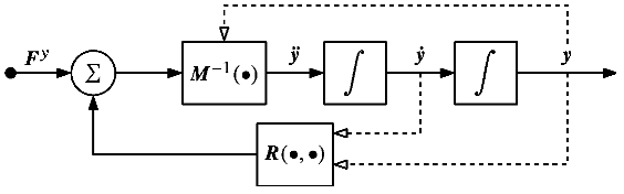
Figure Block diagram for plant dynamics based on the input space ODE of Eq. (24). Solid lines into a block indicate linear arguments and dashed lines represent general nonlinear arguments.
The first example employs the traditional task space approach to track a figure 8 output trajectory for the robot of Fig. 2 with unit values of masses, providing a baseline with which to compare results obtained with the extended operational space formulation. The second example uses the extended operational space formulation with the same output trajectory and zero self-motion, to verify functionality and cyclicity of that formulation. The third example uses both formulations to track the figure 8 output trajectory, while minimizing kinetic energy of the robot mechanism. The fourth example uses the extended operational space formulation to track the figure 8 output trajectory, while avoiding collision with an obstacle.
5.A Traditional Task Space Example
A closed-loop task space controller is investigated for controlling the redundant robot of Fig. The control is applied through generalized force ,
where is the applied task space force in the task space dynamic equation of Eq. (9) [13] . The input of the decoupled system replaces the task acceleration in Eq. (9) and is used to specify a simple proportional-derivative feedback control law,
where is desired output and are proportional and derivative controller gains.
In this and subsequent control examples, it is assumed that the controller has access to perfect estimates of task space dynamic parameters. The task-level feedback controller described by Eqs. (32) and (33) is represented in block diagram form in Fig. Inputs to the controller are the input space state vectors that are used to compute task space coordinates. From these task space coordinates and desired reference signals, an input to the decoupled system is determined and used to estimate the required task space force vector. The output of the controller is the corresponding vector of generalized forces.
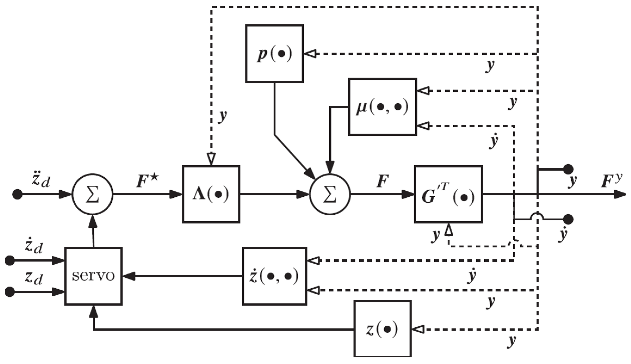
Figure Block diagram for the task space controller based on Eqs. (5), and (31).
This controller can be readily applied to a task space trajectory tracking problem for the robot of Fig. 2 by specifying a desired periodic output trajectory,
The resulting figure 8 task space trajectory that is achieved through the controller of Fig. 4 is shown in Fig. 5 (Left). Controller gains of (proportional) and (derivative) were used. With perfect estimates of the task space parameters, perfect dynamic compensation is achieved and corresponding feedback linearization demonstrates critically damped behavior. The task space feedback controller is able to follow the trajectory of Eq. (34) to arbitrarily high precision. The predicted input trajectory is shown in Fig. 5 (Right). Despite periodicity of the task space trajectory, as shown in Fig. 5 (Left), the task space controller fails to produce cyclic behavior in input space.
Figure 6 (Left) shows a plot of computed input space coordinates versus time. One can examine the degree to which the signals are or are not periodic. Figure 6 (Right) is the image generated in a composite of time frames at regular intervals, relative to the period of the task trajectory. The animation presented in supplemental material gives a visual sense of regularity of the self-motion.
5.An Extended Operational Space Example with Objective
A closed-loop extended operational space controller is specified, in which control is applied through an input space force ,
Denoting estimates of the dynamic parameters using an over hat, the input space acceleration generated from this force is and the operational space acceleration is . With perfect estimates, .
SAs in the previous example, the input of the decoupled system is used to specify a simple proportional-derivative feedback control law. In the extended operational space controller, this term is augmented to include self-motion coordinates, with the objective of achieving the self-motion trajectory ,
With perfect estimates, , where are control gains associated with self-motion coordinates. This yields the linearized error dynamics, , where is the extended operational space error.
The extended operational space feedback controller of Eqs. (35) and (36) can be applied to a task space trajectory tracking problem. It can also be applied to simultaneously track a task space trajectory and a self-motion trajectory. This is demonstrated by specifying a desired self-motion coordinate trajectory in this application, so self-motion coordinates that define robot redundancy appear explicitly in the control implementation of Eq. (36). This contrasts with the traditional task space control implementation in Section 5.1 that does not depend explicitly on robot redundancy. The extended operational space feedback controller defined by Eqs. (35) and (36) is represented in block diagram form in Fig. 7,
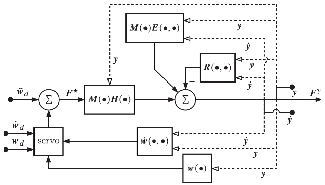
Figure Block diagram for extended operational space feedback controller.
The operational space trajectory achieved through application of the extended operational space controller is shown in Fig. 8 (Left). Controller gains of (proportional) and (derivative) were used. The tracked task trajectory matches the output trajectory generated in the previous example and the v coordinate of is close to zero. The resulting periodic input coordinate trajectory obtained is shown in Fig. 8 (Right). As predicted with periodic output and self-motion, the input space time histories of Fig. 9 (Left) are also periodic. Note that , since . Figure 9 (Right) is the image generated as a composite of time frames at regular intervals relative to the period of the task trajectory. See suplementary material for the animation.
Figure 8.
(Left) Plot of the operational space trajectory produced by the extended operational space controller compared to the reference trajectory. (Right) Input space trajectory showing cyclic behavior.
Figure 8.
(Left) Plot of the operational space trajectory produced by the extended operational space controller compared to the reference trajectory. (Right) Input space trajectory showing cyclic behavior.
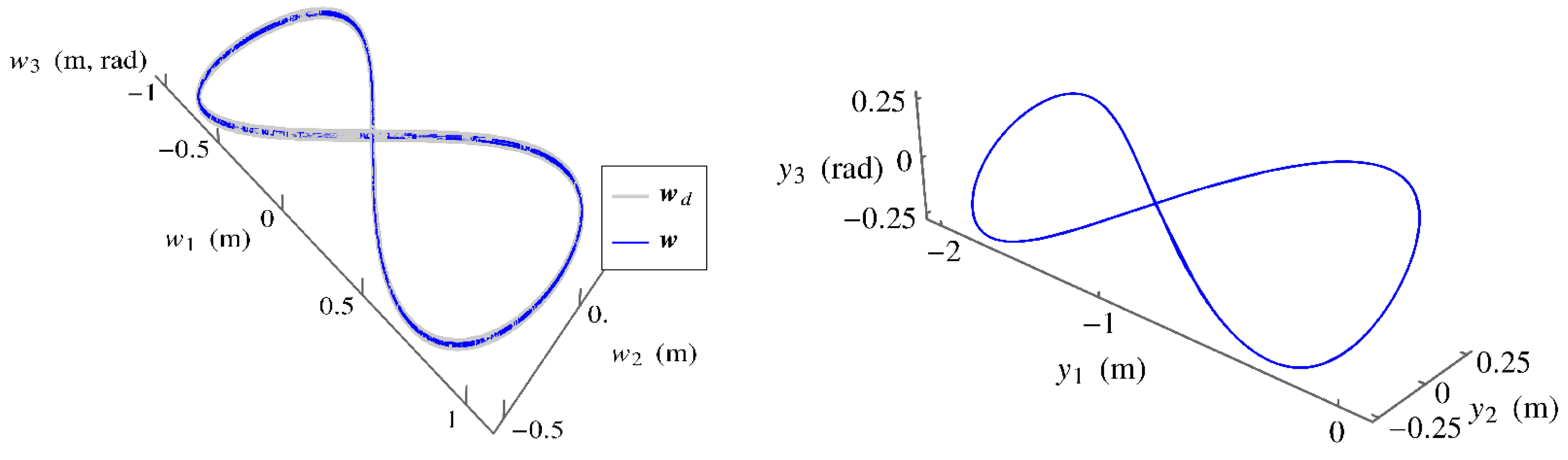
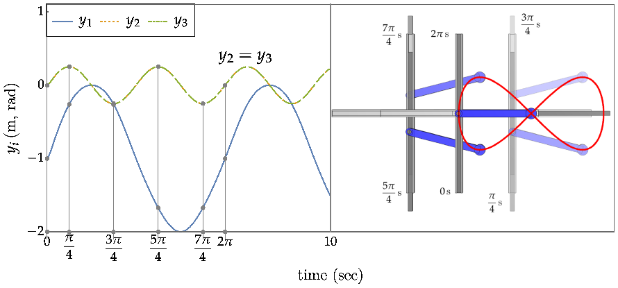
Figure Left) Plot of the input space coordinates versus time. The gray vertical lines and dots indicate key frames at regular intervals relative to the period of the task trajectory. (Right) Key frames composited into a single image, with earlier key frames fading away.
5.An Example with Minimum Kinetic Energy Objective
The intention of this example is to show the effectiveness of minimizing a scalar function, while executing the tracking task, by projecting the gradient of a scalar function along the self-motion coordinates. Minimizing a scalar function by moving along its gradient, within the motion null space, is a common objective in traditional task space control [4].
Both traditional task space and extended operational space control are applied to minimize kinetic energy (scalar function) of the mechanism during execution of the figure 8 tracking task. In the case of traditional task space control, the gradient of kinetic energy is projected onto the null space (local tangent space of the self-motion manifold at an instant), ,
In the case of extended operational space control, the gradient of kinetic energy is multiplied by and concatenated into the term
In implementation of this controller, is evaluated using Eq. (13) that depends explicitly on self-motion coordinates v that represent redundancy of the robot. This is in contrast with the projection in traditional task space control that fails to fully exploit positive aspects of robot redundancy.
Results for the two cases are shown in Fig. Controller gains of (proportional) and (derivative) were used. The expression represents baseline kinetic energy under the figure 8 tracking task, with no null/self-motion space control. The expression represents the case of traditional task space control, with the gradient of kinetic energy projected onto the null space . The expression represents extended operational space control, with the gradient of kinetic energy projected onto the null space . The kinetic energy level with extended operational space control, , is much lower than the baseline case. More significantly, is reduced with respect to . For animation of results, see supplementary materials.
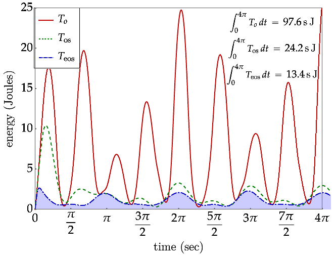
Figure Plots of kinetic energy versus time. represents the case of traditional task space control, with the gradient of kinetic energy projected onto the null space . represents the case of extended operational space control, with the gradient of kinetic energy projected onto the null space .
It is important to note that a dynamically consistent generalized inverse of the task Jacobian is defined [13] to minimize kinetic energy of the solution of the velocity kinematic equation,. In fact, the dynamically consistent inverse is a mass weighted version of the Moore-Penrose inverse that has the property of yielding the least velocity norm solution. The mass weighted inverse solution of the velocity equation is precisely the least kinetic energy (analogous to least norm). Despite this property of the dynamically consistent inverse, it can be seen in Fig. 10 that it does not produce minimal kinetic energy over a time series. In retrospect, it should not be expected to do so, since the kinetic energy property that it satisfies is an instantaneous one that is dependent upon the specific configuration. There is no guarantee that self-motion configurations that the path follows are consistent with low kinetic energy relative to other paths.
5.An Extended Operational Space Example with Obstacle Avoidance
Obstacle avoidance (particularly using artificial potential fields) is another common application for redundant robots. It is relevant to present an example with this approach in order to characterize the utility of implementing the artificial potential field approach within the extended operational space formalism. An obstacle is introduced into the robot workspace that is to be avoided by the top of the vertical guiderail of the robot, as shown in Fig. The task space controller is used to track the figure 8 output. Controller gains of (proportional) and (derivative) were used. Rather than tracking a specific trajectory in the self-motion space, a reactive artificial potential field control is applied to avoid the obstacle, with input to the self-motion space. A repulsive artificial potential field is used, of the form
where is a constant coefficient and is the distance function. The constant is the offset to the top of the vertical guide rail; i.e., the point on the robot for which obstacle avoidance is specified. From left to right in Fig. 11, the obstacle descends downward and then levels off. The point of influence for the robot is the top of the vertical guide rail. The field gradient is applied as control input into the self-motion space. Figure 11 (Right) depicts the obstacle wrapped within the potential field.
In the input of the decoupled system, the self-motion space tracking term is replaced by the (negative) gradient of the potential field , pre-multiplied by . This defines
that depends on self-motion coordinate v through its influence on of Eq. (13). The controller block diagram for this application is shown in Fig. 12.
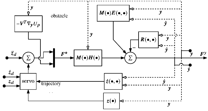
Figure Block diagram of a controller, specifying task space trajectory tracking and artificial potential field obstacle avoidance in the self-motion manifold.
Results of the output trajectory tracking problem with simultaneous obstacle avoidance are shown in Figs. 13 and The orange line in Fig. 14 is the trace of the upper tip of the vertical guide rail, which is the point of application of the repulsive potential field. The obstacle avoidance control dynamically decouples from the task trajectory control, due to its point of application within the self-motion space. Since the self-motion trajectory generated is not periodic, there is no reason to believe that the input trajectory obtained will be periodic; i.e., the robot will not be cyclic in this control generated motion. Nevertheless, in the left plot of Fig. 13 is nearly constant and z is periodic, so the joint displacements of Fig. 13 (Right) are nearly cyclic, as seen in annimations.
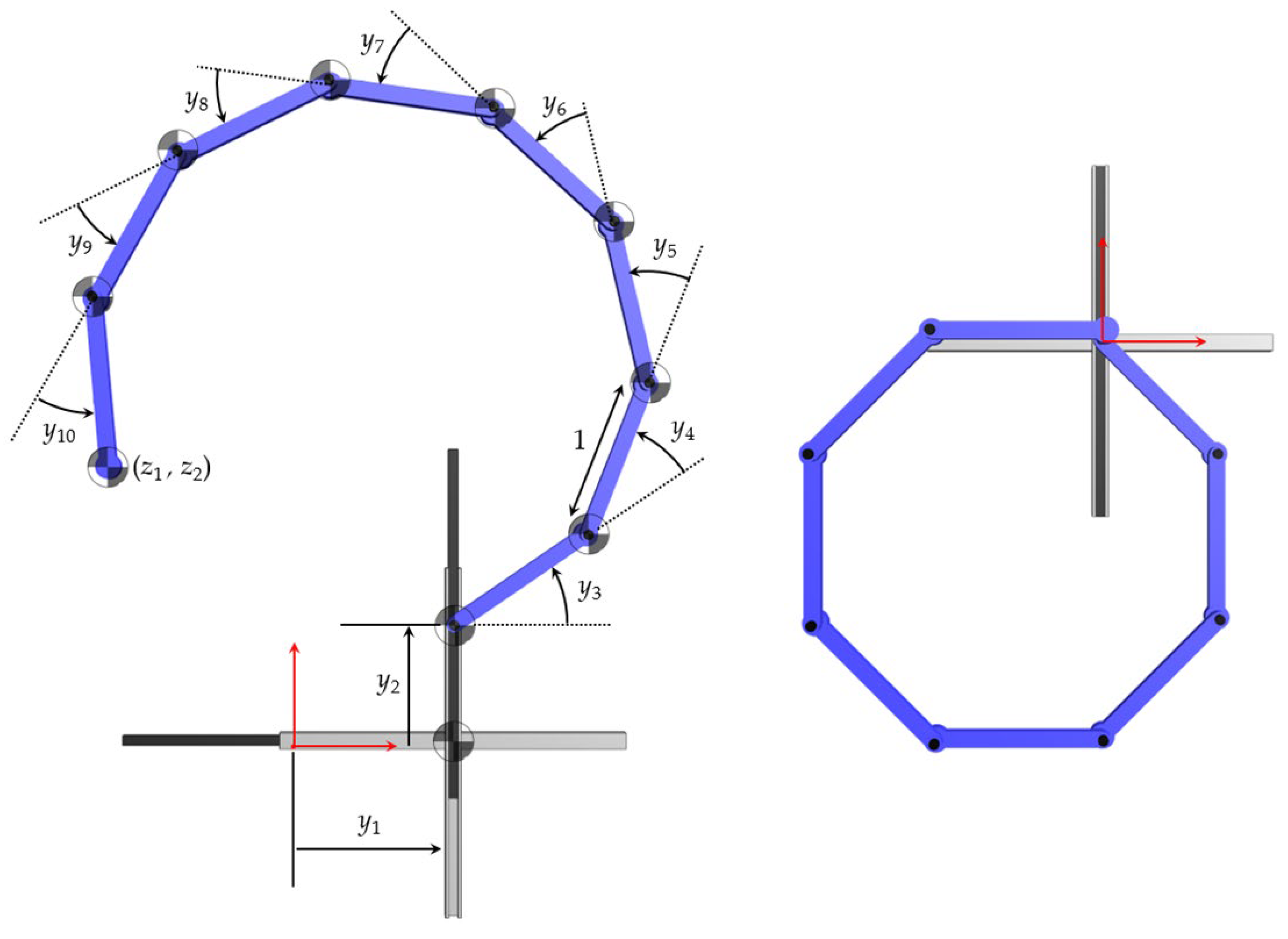
An Eight Degree of Redundancy Test Problem
The planar manipulator of Fig. 15 (Left) with 8 unit length members has ten input coordinates and two output coordinates . Its kinematic equation is
.
with Jacobian where is the k-th column of the Jacobian (), with defined as . In addition to its analytical simplicity, this is an attractive example for analysis, since the Jacobian matrix of is of full rank throughout manipulator configuration space. Any pathological behavior of the manipulator cannot, therefore, be attributed to a rank deficient Jacobian.
To obtain input space ODE of motion for this manipulator, point masses are defined at the end of each link, with the global positions , , and , where and . The ODE of motion of Eq. (24) in input space are given by the matrices , , and , where is the Jacobian of with respect to and g = 9.80665 m/s2 is the acceleration of gravity, pointing downward in Fig. In the following, two operational space controllers will be compared to track the following desired task trajectory:
For both traditional and extended operational space control, initial conditions of the manipulator are and . This initial configuration of the manipulator is shown in Fig. 15 (Right).
6.Traditional Operational Space Control
The first test is with the traditional task space controller, causing the end-effector of the manipulator to follow the desired trajectory of Eq. (41) with no gravitational effects; i.e., neglecting the term of Eq. (24). This assumes that the manipulator moves in a horizontal plane, perpendicular to the gravity vector. The traditional task space controller projects the dynamics of the manipulator to its task space z by means of
where , , and . A Computed-Torque Control (CTC) law for [26] that achieves asymptotic tracking of desired trajectories for the output variables can be constructed by substituting for in (42) an defined as . This can be transformed to generalized input control forces through G′T
,. Gains and can be selected to achieve the desired tracking with the desired dynamic performance. Values and are selected to cause the tracking error to converge to zero asymptotically, with a critically damped behavior and a settling time of ≈0.5 seconds. This means that 95% of the error will be removed in 0.5 seconds. Application of the controller given by Eq. (42) generates the results shown in Fig. 16, in which one can observe that the input time history is not cyclic . Attached animations emphasize this behavior.
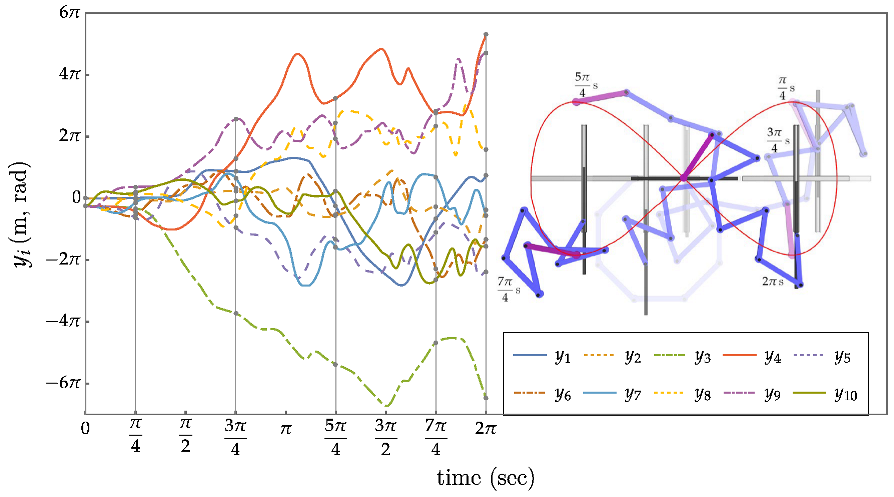
Figure Control results using the Traditional Operational Space controller. Non-cyclic evolution of input coordinates (Left). Some snapshots of the manipulator executing the desired task trajectory (Right).
6.Extended Operational Space Control
For the extended operational space controller, the parameterization is initialized at with evaluated using Eq. (10) and initial 0. With these values and matrices of Section 3.2, the following control law is defined
where
and the desired trajectory for is 0. Gains are chosen as , , and .
Application of this controller generates the results shown in Fig. 17, where gravity has been suppressed. Comparing this result with Fig. 16, it is seen that the extended operational space controller not only achieves cyclic behavior in the inputs, but also generates a much smoother and lower magnitude input, compared to the wilder variation of inputs in Fig. An even greater contrast in behavior of the two control approaches is provided by the kinetic energy plots in Fig. 18. Clearly the motion generated by the traditional task space approach is the more extreme. To better appreciate the distinct dynamic nature of the motions, see the attached animations. Despite the large motion experienced by the manipulator Fig. 17, the initial basis () was valid during the entire trajectory, without having to reparametrize due to rank deficiency of .
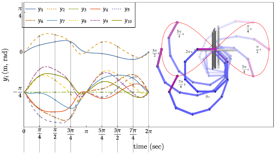
Figure Control results using the Extended Operational Space controller. Cyclic evolution of input coordinates after one cycle of the output variables (Left). Some snapshots of the manipulator executing the desired trajectory (Right).
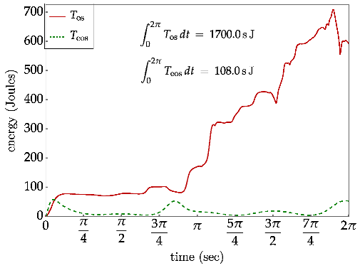
Figure Kinetic Energy of Traditional Task Space and Extended Operational Space Controlled Robots vs Time.
Interestingly, setting the second row of to zero in Eq. (44), which corresponds to the CTC controller [26] for , yields exactly the same results of Fig. This means exerting no control at all on the dynamics of ; i.e., leaving them unactuated. This works only because the desired evolution for coincides with their initial value (0), their initial velocities are zero, and there are no external forces like gravity perturbing their dynamics, so they can be left unactuated while controlling only . If gravity is considered, then it is necessary to keep the second row of
F⋆ to achieve the desired control.
Conclusions and Recommendations for Future Research
The extended operational space kinematics, dynamics, and control formulation presented is applicable to a broad spectrum of redundant serial robots. The analytical form of robot inverse kinematics presented depends explicitly on self-motion coordinates that represent robot redundancy. This corrects fundamental errors in generalized inverse velocity kinematics formulations that have been used in the redundant robot literature for over half a century. The extended operational space ODE obtained, in terms of output and self-motion coordinates, quantitively represent robot redundancy and are ideally suited for robot control. Further research is needed in defining singularity free subdomains of the extended operational configuration space. Following the approach presented herein, recent results on redundant robot kinematics and dynamics of non-serial robots [27,28] may be extended, for control of non-serial robots.
Based on the extended operational configuration space ODE presented, a robot control architecture is defined that exploits the potential offered by redundant serial robots, using self-motion coordinates that characterize robot redundancy. Four one degree of redundancy applications are presented in Section 5 that demonstrate accuracy and functionality of the control architecture, including output trajectory tracking while minimizing system kinetic energy and avoiding obstacles. Using traditional task space tracking control as a baseline, comparisons are made between task space and extended operational space control. For the figure 8 tracking task, both the task space controller and the extended operational space controller perform the tracking task, without any visible error. Both controllers exploit knowledge of system dynamics in the feed-forward path and the same modest proportional-derivative gains in the feedback path. The combination leads to feedback linearization and critically damped behavior. Robustness to plant estimates and disturbances is to be assessed in the future.
The self-motion control in examples presented in Section 5 demonstrates classic dynamic decoupling between task and self-motion spaces. This is not surprising, since it is included by design in both the traditional task space formulation and the extended operational space formulation. However, the extended operational space formulation provides a means for exploiting self-motion coordinates that represent robot redundancy, an option that is not available in previous redundant serial robot kinematics formulations. As noted, in the traditional task space approach, there are no explicit coordinates that span the self-motion space, only an instantaneous tangent space. Consequently, task space self-motion control is limited to projecting a vector quantity of interest onto a linear space that is decoupled from the task control. The extended operational space approach is especially effective in gradient based minimization of desired quantities, performing these minimizations better than the task space approach. Tracking of self-motion coordinates was done easily and with great fidelity, which could not be done with traditional task space control.
Further comparison between traditional and extended formulations applied to an eight degree of redundancy robot in Section 6 shows that controllers based on the traditional task space formulation produce larger variations of internal self-motion than the extended operational space formulation. The new formulation moderates self motion under control, while preserving cyclicity of the configuration under specified cyclic task space trajectories. This is illustrated in both animations of the manipulator and in the comparison of mechanism kinetic energy in Fig. 18.
While an extended operational space adaptation of feedback linearization was successfully employed, future work will consider more sophisticated control approaches. Among these are the use of Model Predictive Control (MPC) [29] to find globally optimal control inputs, as well as approaches such as sliding mode control to improve robustness to internal modeling errors and external disturbances.
Supplementary Materials
The following supporting video information can be downloaded at the website of this paper posted on: Preprints.org; fig6sup, fig6sup, fig9sup, fig10sup, fig14sup, fig16sup, fig17sup.
Author Contributions
EH and VD conceived and designed the study. EH developed the differential geometry results. VD and AP developed the control results. EH, VD, and AP wrote the article.
Financial Support
This research received no specific grant from any funding agency, commercial or not-for-profit sectors.
Conflicts of Interest
The authors declare no conflicts of interest exist.
References
- Chiaverini, S., Oriolo, G., and Maciejewski, A. A., Redundant Robots, Siciliano and Khatib eds, Springer Handbook of Robotics, 2nd ed, Springer-Verlag Berlin, 2016.
- Whitney, D. E., Resolved Motion Rate Control of Manipulators and Human Prostheses, IEEE Transactions on Man-Machine Systems, 1969, Vol.10, No. 2, pp. 47-53. [CrossRef]
- Haug, E. J., Redundant Serial Manipulator Inverse Position Kinematics and Dynamics, Journal of Mechanisms and Robotics, 2024, Vol. 16, p. 081008. [CrossRef]
- Khatib, O., A Unified Approach for Motion and Force Control of Robot Manipulators: The Operational Space Formulation”, IEEE Journal of Robotics and Automation, 1987, Vol. RA-3, No. 1, pp. 43-53. [CrossRef]
- Nakanishi, J., Cory, R., Mistry, M., Peters, J., and Schaal, S., Operational Space Control: A Theoretical and Empirical Comparison, The International Journal of Robotics Research, 2008, Vol. 27, No. 6, pp. 737-757. [CrossRef]
- Park, K. C., Chang, P.-H., and Lee, S., Analysis and control of redundant manipulator dynamics based on an extended operational space, Robotica, 2001, Vol. 19, pp. 649-662. [CrossRef]
- De Sapio, V., Advanced Analytical Dynamics, Cambridge University Press, Cambridge, UK, 2017.
- Haack, W., and Wendland, W., Lectures on Partial and Pfaffian Differential Equations, Pergamon Press, Oxford, UK, 1972.
- De Luca, A., and Oriolo, G., Nonholonomic Behavior in Redundant Robots Under Kinematic Control, IEEE Transactions on Robotics and Automation, 1997, Vol. 13, No. 5, pp. 776-782. [CrossRef]
- Shamir, T., and Yomdin, Y., Repeatability of Redundant Manipulators: Mathematical Solution of the Problem, IEEE Transactions on Automatic Control, 1988, Vol. 33, No. 11, pp. 1004-1009. [CrossRef]
- Haug, E. J., A Cyclic Differentiable Manifold Representation of Redundant Manipulator Kinematics, Journal of Mechanisms and Robotics, 2024, Vol. 16, p. 061005. [CrossRef]
- Klein, C. A., and Huang, C.-H., Review of Pseudoinverse Control for Use with Kinematically Redundant Manipulators, IEEE Transactions on Systems, Man, and Cybernetics, 1983, Vol. SMC-13, No. 3, pp. 245-250. [CrossRef]
- Khatib, O., Inertial Properties in Robotic Manipulation: An Object-Level Framework, The International Journal of Robotics Research, 1995, Vol. 13, No. 1, pp. 19-36. [CrossRef]
- Deo, A., and Walker, I., Overview of Damped Least- Squares Methods for Inverse Kinematics of Robot Manipulators, Journal of Intelligent Robotic Systems, 1995, Vol. 14, No. 1, pp. 43-68. [CrossRef]
- Hogan, N., Impedance Control: An Approach to Manipulation: Part I - Theory, Part II - Implementation, Part III – Applications, Journal of Dynamic Systems, Measurement, and Control, 1985, Vol. 107, No. 1, pp. 1-24. [CrossRef]
- Hollerbach, J., and Suh, K. C., Redundancy Resolution of Manipulators Through Torque Optimization, IEEE Journal of Robotics and Automation, 1987, Vol. RA-3, No. 4, pp. 308–316. [CrossRef]
- Simas, H., and Di Gregorio, R., A Technique Based on Adaptive Extended Jacobians for Improving the Robustness of the Inverse Numerical Kinematics of Redundant Robots, Journal of Mechanisms and Robotics, 2010, Vol. 11, p. 020913.
- Dietrich, A., Ott, C., and Albu-Schäeffer, A., An Overview of Null Space Projections for Redundant, Torque-Controlled Robots, The International Journal of Robotics Research, 2015, Vol. 34, No. 11, pp. 1385-1400. [CrossRef]
- Haug, E. J., Computer-Aided Kinematics and Dynamics of Mechanical Systems, Volume II: Modern Methods, Fourth Ed., Amazon.com, 2024.
- Lee, J. M., Introduction to Smooth Manifolds, Second Ed., Springer, New York, 2013.
- Robbin, J. W., and Salamon, D. A., Introduction to Differential Geometry, Springer, Berlin, 2022.
- Atkinson, K. E., An Introduction to Numerical Analysis, Second Ed., Wiley, New York, 1989. [CrossRef]
- Corwin, L. J., and Szczarba, R. H., Multivariable Calculus, Marcel Dekker, New York, 1982.
- Haug, E. J., and Peidro, A., Redundant Manipulator Kinematics and Dynamics on Differentiable Manifolds, Journal of Computational and Nonlinear Dynamics, 2022, Vol. 17, p. 111008. [CrossRef]
- Peidro, A., and Haug, E. J., Obstacle Avoidance in Operational Configuration Space of Kinematically Redundant Serial Manipulators, Machines, 2024, Vol. 12, No. 10. [CrossRef]
- Chung, W. K., Fu, L. C., and Kröger, T., Motion control, In Siciliano, B, and Khatib, O, (eds), Springer Handbook of Robotics, 2016, Springer-Verlag, Berlin, pp. 174-177.
- Haug, E. J., Redundant Non-Serial Implicit Manipulator Kinematics and Dynamics, Journal of Mechanisms and Robotics, 2024, Vol. 16, p. 061017. [CrossRef]
- Haug, E. J., Redundant Non-Serial Compound Manipulator Kinematics and Dynamics, Mechanism and Machine Theory, 2024, Vol. 200, p. 105717. [CrossRef]
- Nicolis, D., Allevi, F., and Rocco, P., Operational space model predictive sliding mode control for redundant manipulators, IEEE Transactions on Robotics, 2020, Vol. 36, No. 4, pp. 1348-1355. [CrossRef]
Figure 2.
(Left) Redundant serial robot schematic. (Right) Robot mechanism structural rendering annotated with link axes, centers of mass, and joint displacements.
Figure 2.
(Left) Redundant serial robot schematic. (Right) Robot mechanism structural rendering annotated with link axes, centers of mass, and joint displacements.
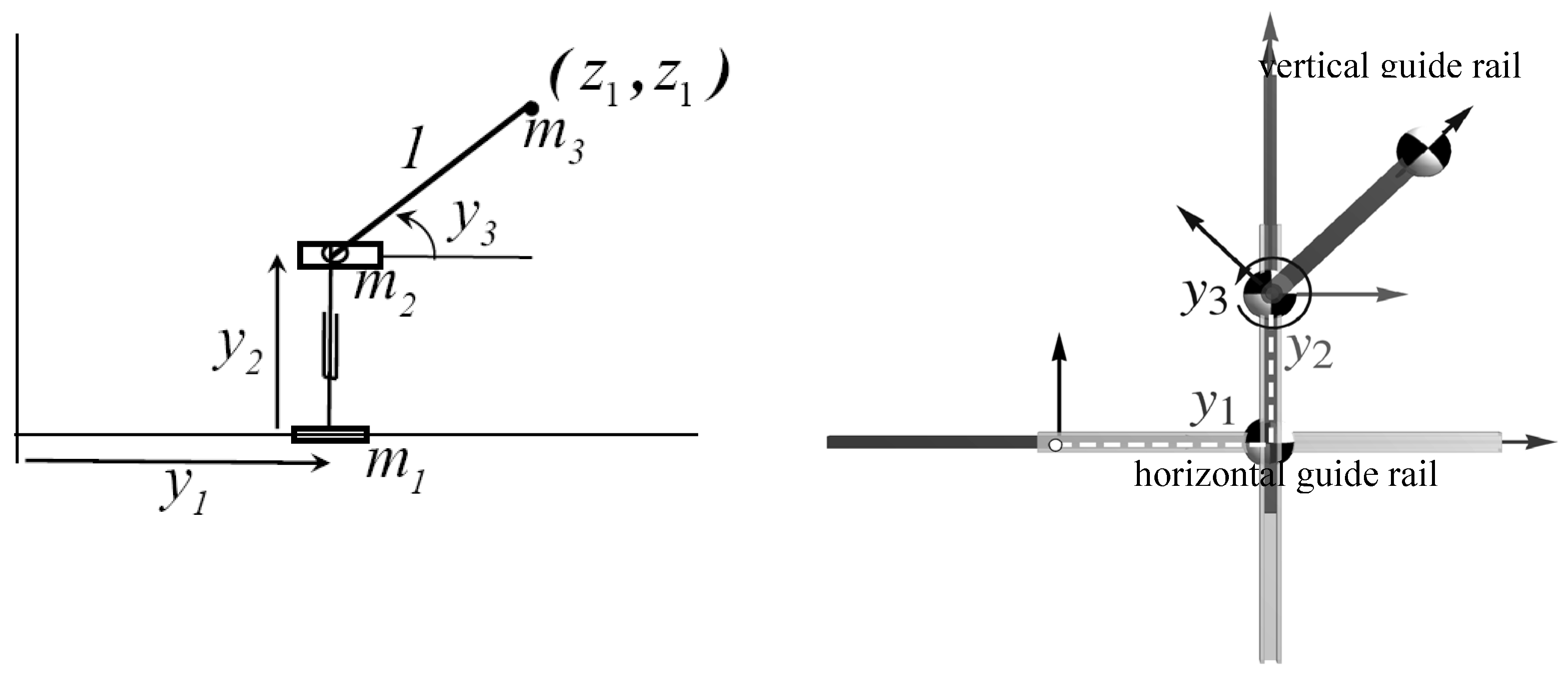
Figure 5.
(Left) Plot of trajectory produced by the task space controller compared to the reference trajectory. (Right) Input space trajectory showing acyclic behavior despite periodic task trajectory.
Figure 5.
(Left) Plot of trajectory produced by the task space controller compared to the reference trajectory. (Right) Input space trajectory showing acyclic behavior despite periodic task trajectory.
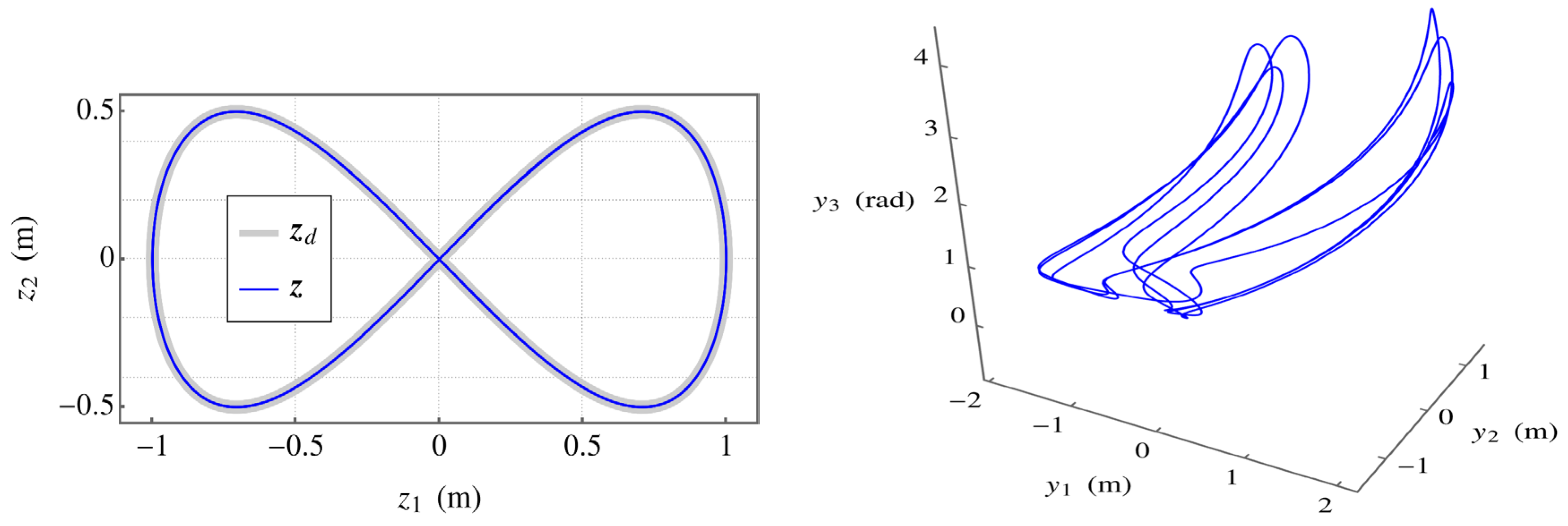
Figure 6.
(Left) Plot of the input space coordinates versus time. The gray vertical lines and dots indicate key frames at regular intervals relative to the period of the task trajectory. (Right) Key frames composited into a single image, with earlier key frames fading away. Times are shown.
Figure 6.
(Left) Plot of the input space coordinates versus time. The gray vertical lines and dots indicate key frames at regular intervals relative to the period of the task trajectory. (Right) Key frames composited into a single image, with earlier key frames fading away. Times are shown.
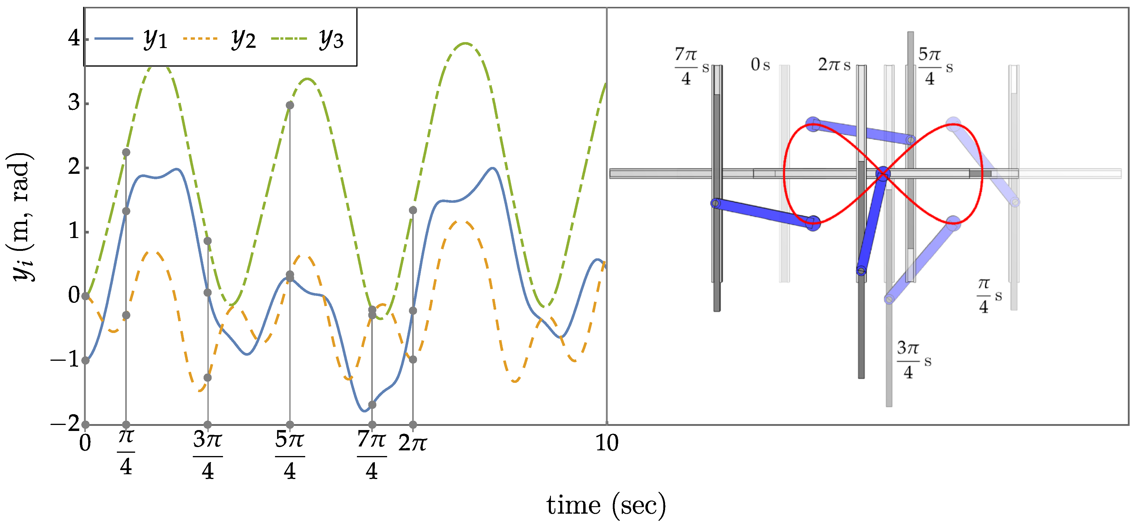
Figure 11.
(Left) Overhead obstacle present in robot workspace. (Right) Robot depicted under the influence of a repulsive potential field.
Figure 11.
(Left) Overhead obstacle present in robot workspace. (Right) Robot depicted under the influence of a repulsive potential field.
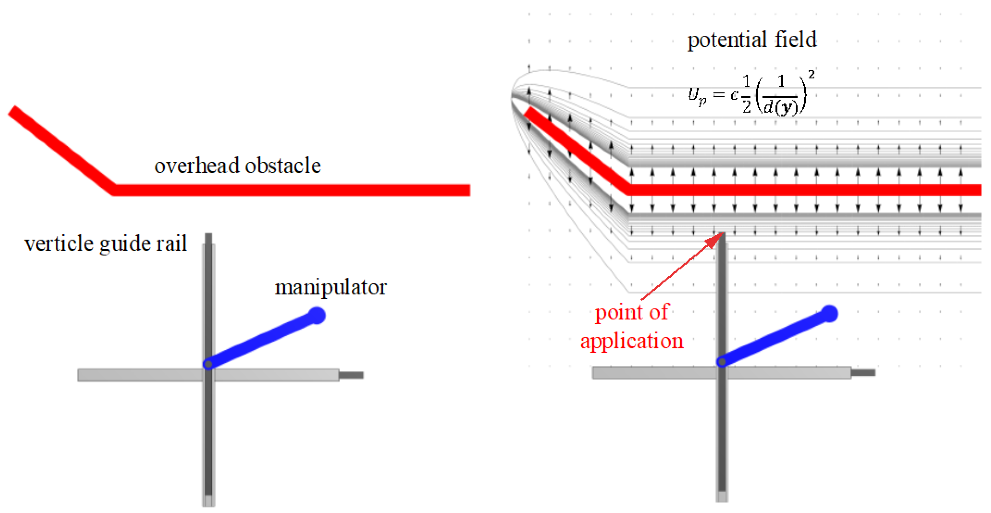
Figure 13.
(Left) Plot of the operational trajectory produced by the extended operational space controller compared to the reference trajectory. (Right) Input space trajectory showing slightly acyclic behavior.
Figure 13.
(Left) Plot of the operational trajectory produced by the extended operational space controller compared to the reference trajectory. (Right) Input space trajectory showing slightly acyclic behavior.
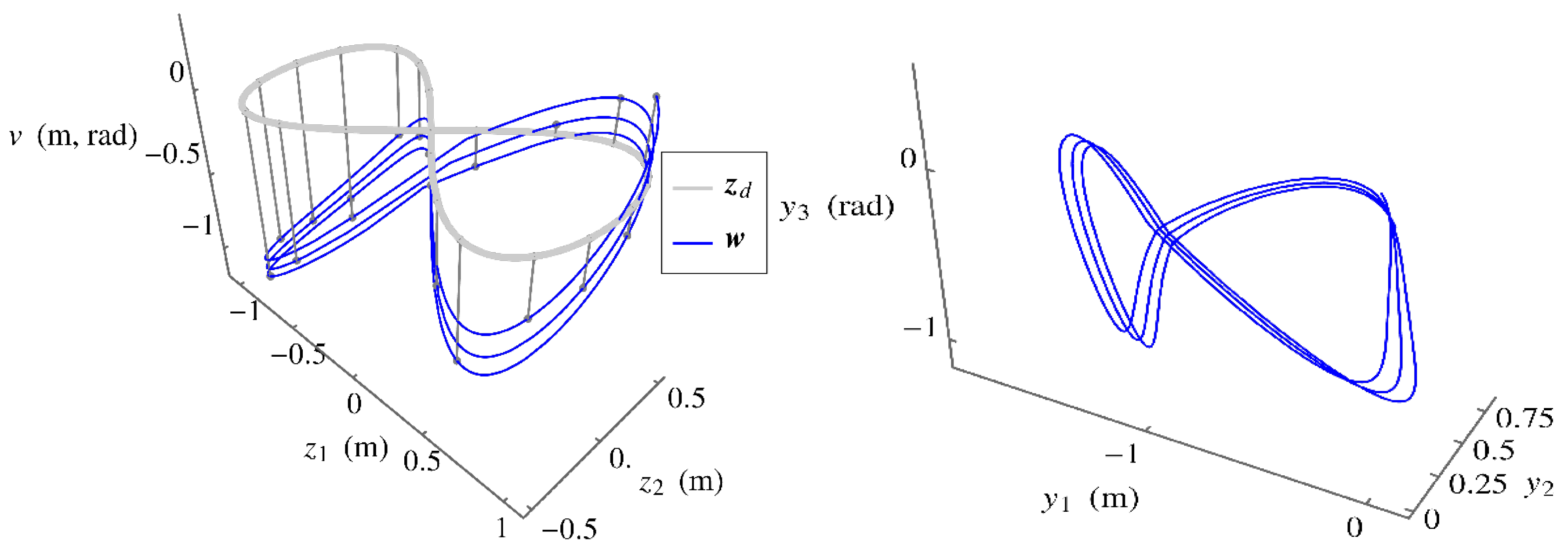
Figure 14.
(Left) Plot of the input space coordinates versus t. (Right) Composite frame image (see animation in supplementary material).
Figure 14.
(Left) Plot of the input space coordinates versus t. (Right) Composite frame image (see animation in supplementary material).
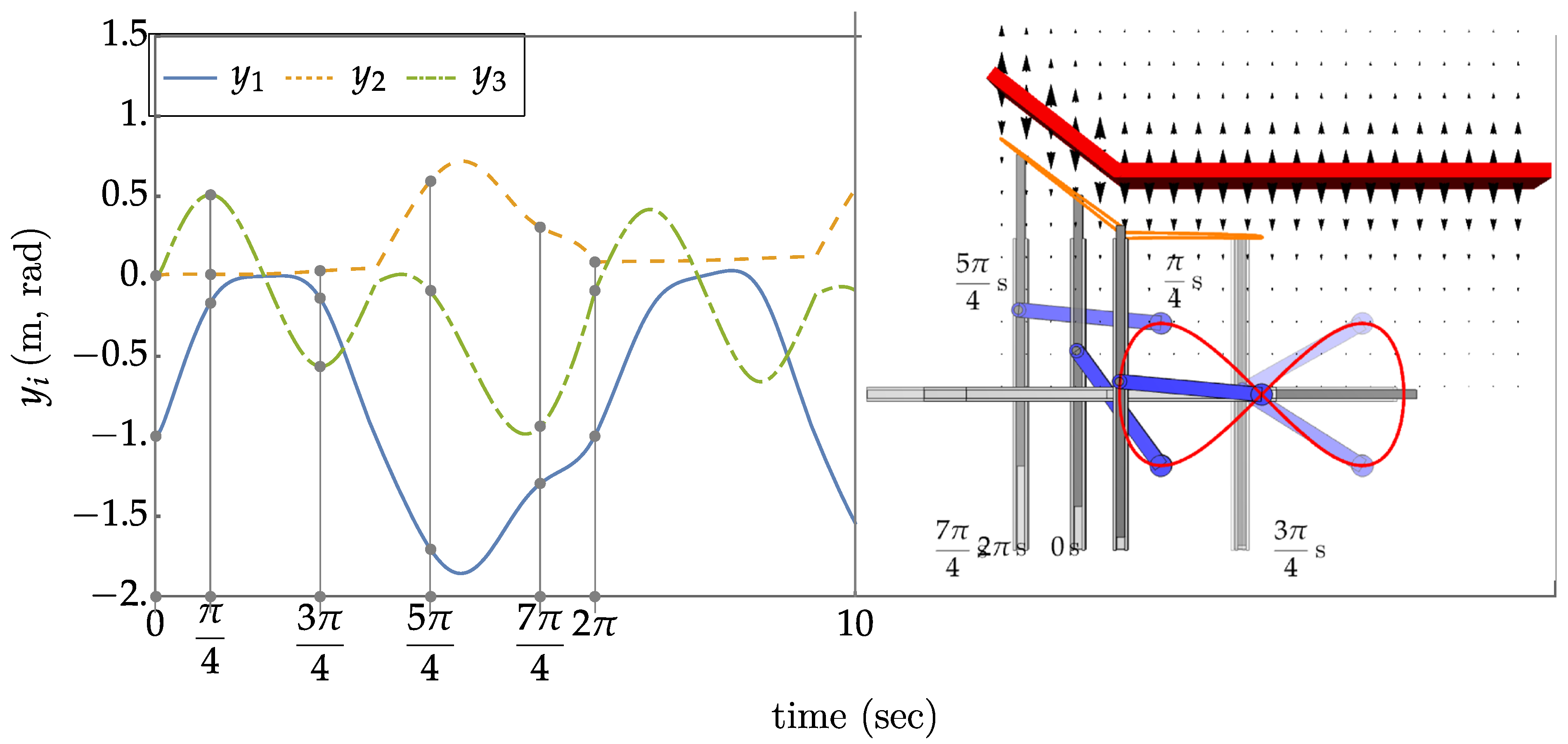
Figure 15.
(Left) Manipulator mechanism structural rendering annotated with link axes, centers of mass, and joint displacements. (Right) Initial configuration
Figure 15.
(Left) Manipulator mechanism structural rendering annotated with link axes, centers of mass, and joint displacements. (Right) Initial configuration
Disclaimer/Publisher’s Note: The statements, opinions and data contained in all publications are solely those of the individual author(s) and contributor(s) and not of MDPI and/or the editor(s). MDPI and/or the editor(s) disclaim responsibility for any injury to people or property resulting from any ideas, methods, instructions or products referred to in the content. |
© 2024 by the authors. Licensee MDPI, Basel, Switzerland. This article is an open access article distributed under the terms and conditions of the Creative Commons Attribution (CC BY) license (http://creativecommons.org/licenses/by/4.0/).
Copyright: This open access article is published under a Creative Commons CC BY 4.0 license, which permit the free download, distribution, and reuse, provided that the author and preprint are cited in any reuse.


