Submitted:
25 October 2024
Posted:
28 October 2024
Read the latest preprint version here
Abstract
The rising popularity of UAVs and other autonomous control systems, coupled with real-time operating systems, has increased the complexity of developing systems with the proper robustness, performance, and reactivity. Concurrently, the growing demand for more sophisticated computational tasks, proportionally bigger payloads, battery limitations, and smaller take-off mass necessitates higher energy efficiency for all avionics and mission computers. The purpose of this paper is to develop the technology for experimental studies of indicators of reactivity and energy consumption of the computing platform for unmanned aerial vehicles (UAVs). The paper provides an experimental assessment of the ’Boryviter’ 0.1 computing platform, which is implemented on the ATSAMV71 microprocessor and operates under the open-source FreeRTOS operating system. The results obtained are the basis for developing algorithms and energy-efficient design strategies for the mission computer to solve the optimization problem. The paper provides experimental results of measurements of the energy consumed by the microcontroller and estimates of the reduction in system energy consumption due to additional time costs for suspending and resuming the computer’s operation. The results show that the ’Boryviter’ 0.1 computing platform can be used as a UAV mission computer for typical flight control tasks that require real-time computing under the influence of external factors. As the further work direction, authors plan to carry out the investigation of the proposed energy saving algorithms in scope of the planned NASA’s F’Prime software flight framework. Such an investigation that should be done with the real flight computation load for the mission computer, will help to qualify the obtained energy saving methods and their implementation results.
Keywords:
UAV
; mission computer
; software
; Boryviter
; Falco
; computational efficiency
; overhead costs
; energy efficiency
; reactivity
; ATSAMV71
; FreeRTOS
; earliest deadline first
; rate monotonic scheduling
; low power modes
1. Introduction
Today, unmanned aerial vehicles (UAVs) are widely used in many areas of human activity and play an essential role in scientific, industrial, search and rescue, surveillance, cinematographic and other tasks [1]. The use of UAVs made it possible to carry out dangerous missions without risking the health and life of the operators. With the beginning of Russia’s aggression in Ukraine, it became clear that the effective use of UAVs on the battlefield was almost the only possibility for the Ukrainian armed forces to oppose Russia’s massive military machine. Analyzing this confrontation, the Center of Excellence for Integrated Air and Missile Defense in the report [2] emphasizes the need to adapt NATO’s military doctrines, concepts, and tactics to the new realities of using UAVs, UGVs (unmanned ground vehicles), UWVs (unmanned water vehicles/vessels) and countermeasure systems.
The works [3,4] present an overview of UAV research and highlight the latest trends and achievements. The authors also consider UAVs’ general hardware and software architecture and describe their applications. The article [5] provides an overview and classification of UAVs. It also describes the capabilities and characteristics of UAVs weighing 2 to 11,600 kg and operating up to 40 hours.
The UAV market is actively developing. According to Fortune Business Insights [6], the CAGR of the global UAV market is 16.3% for the period 2023-2030, and the majority of the market is accounted for by UAVs of small and tactical devices (Figure 1). For such UAVs, the requirements for the on-board computer must correspond to the increased complexity of the system [7,8,9,10].
Every UAV that takes off has its mission to generate value for the operator of a UAV. To carry out its mission, a UAV shall consist of reliable, powerful, and yet power-efficient avionics (Figure 2) with the required mission capabilities. The orchestration of the mission is done by a central computer, which is called the mission computer. The typical tasks of the mission computer are to control the entire avionics, compute the UAV’s route, ensure communication to the ground station (if required), and control the onboard payload.
This article will concentrate on the mission computer alone as this is the most complex yet flexible and configurable part of modern UAV avionics.
The background of the research in this paper is the growing need for real-time mission computers that are powerful and responsive yet power-efficient and cost-efficient.
Investigating the trade-off between system reactivity and the use of energy-saving modes of the computing platform is vital in many situations, not only for UAVs but also in all real-time systems with an autonomous power supply. These are embedded systems in industrial applications, Internet of Things (IoT) devices, implanted medical devices, emergency notification systems, etc. During the operation of the computing platform, this compromise is achieved through software-implemented algorithms that allow adaptive control of computer operating modes depending on current conditions and requirements for reactivity and energy consumption of the system. To solve the question of the expediency of spending on the development of new algorithms and software, an experimental study is needed to build a mathematical model that comprehensively characterizes the reactivity and energy consumption of the computer.
The purpose of this paper is to develop a technique for experimental studies of indicators of reactivity and energy consumption of the computing platform for UAVs. All work in the paper is carried out using the authors’ mission computer ’Boryviter 0.1’.
The paper is structured as follows:
- Chapter 2 - ’Domain Overview,’ introduces the reader to the mission of computers as the object of the study, provides an overview of the real-time operation systems (RTOS) usage challenges, and describes tools and needs of energy-saving solutions for embedded mission computers;
- Chapter 3 - ’Materials And Methods’ describes the platform for conducting the study experiment, defines a system model in the look of a power state machine, and describes the exact way of measuring reactivity and power consumption of different modes of operation;
- Chapter 4 - ’Results’ provides the obtained experiment results;
- Chapter 5 - ’Discussion’ describes and presents the obtained results applied to the proposed system model;
- Chapter 6 - ’Conclusion’ concludes the article by describing the novelty of the research and its further development.
2. Domain Overview
The chapter provides an extensive overview of the technology, design, and efficiency considerations for mission computers in unmanned aerial vehicles (UAVs).
The modern approach for the avionics and mission computers development consists of the following key steps:
- Select an appropriate ready-to-use avionics platform (including a mission computer);
- Use microcontroller-specific vendor toolchain;
- Ensure that a real-time operation system is in place and can be easily adapted to the selected computation platform;
- Design and validate the required for the flight mission business logic (i.e. what exactly a UAV shall do).
All of the items above do not guarantee that the selected platform, microcontroller, operating system, and other components will allow the integrator to achieve the required results to fulfill the mission objectives. In the chapter, an in-depth review of the technologies, techniques, parts, and problems mentioned in the UAV avionics design process is reviewed.
2.1. UAV Avionics and Mission Computers
Typical UAV avionics (the on-board electronics) consist of several parts, they are (Figure 3):
- Mission computer (often called an on-board computer or flight controller board);
- Navigation and orientation system (GNSS and GPS);
- Sensors board + sensors;
- Remote control and telemetry system (Communication unit);
- Energy and propulsion system (Driving unit);
- Payload (sometimes called an off-board module).
A mission computer is a specialized computer system integrated into the avionics of a UAV or, in general, into another complex technical device that requires autonomous control and high reliability[12]. Computational power, reactivity, energy efficiency, peripheral support, and real-time performance are important considerations when choosing a mission computer. The reality of mission computer build-up and development shows that most commercial off-the-shelf (COTS) products [13] are built on a specific series of microcontrollers or microprocessors (main processors) known to the development team or the vendor. This expertise significantly advances software quality, expedites time-to-market, and enhances flight heritage.
Microcontroller units (MCUs) utilized in UAVs or nanosatellites generally exhibit substantial similarities, except when considering radiation-hardened or radiation-tolerant microcontrollers [14]. These specific microcontrollers are beyond the affordability of commercial electronics and, consequently, will not be evaluated in this article. As a result, the spectrum of available components for utilization, as well as the associated toolchain for RTOSes and development tools, is considerably broadened.
The similarity of the requirements for the construction of UAV and nanosatellites onboard systems makes it expedient to use a standard technology stack [15] to address both application areas being part of aerospace engineering. A description of the highly integrated onboard computing products used for CubeSat missions (class of nanosatellites) is given in [16]. The most energy-saving solutions are based on ARM Cortex-Mx (where x is 0 to 7), LEON3FT, and Atmel ARM 9.
Electronic component manufacturers constantly update available offers, allowing UAV developers to achieve better results (appropriate productivity with low power consumption) when solving complex tasks. Popular MCU series with brand new families that can be used in UAV onboard systems include the SAMx Series (Atmel/Microchip) [17], PIC32 (Microchip), STM32 Series (STMicroelectronics) and iMX.RT series (NXP). The characteristics of the popular series of 32-bit microcontrollers for implementing UAV mission computers are listed in Table 1. The precise selection of the components examined was determined by balancing between performance, available memory, and the availability of energy-saving modes.
2.2. Problems and Researches in the Field of Mission Computers
Ensuring the ability to fly autonomously requires efficient sensor operation, appropriate flight control, and mission software. There is a lot of research on using AI for these tasks, such as computer vision for object recognition and tracking [18,19,20], reinforcement learning for mission control [21], sensor fusion, and others. The success of missions in general and, in particular, the effectiveness of the application of machine learning (ML) models critically depends on the reactivity of the onboard system to ensure the prompt acquisition of data and the speed of execution of the relevant program blocks.
Another area of research is the energy efficiency [15,22] of the onboard systems, which directly affects the maximum duration of the UAV flight with the maximum reduction of the weight of the powertrain and its energy source. Any calculations, from the business logic that performs the business tasks (payload) and overall mission control (such as engine control) to system ones, such as diagnosing the state of the computer and connected sensors and actuators, require software running on the central processor or microcontrollers. The availability of microcontrollers does not play the last role in the selection of electronic components for mission computers. Research is being conducted on the experimental comparison of the solution’s effectiveness based on various technology stacks, which involve using budget solutions and open-source software. Thus, the paper [23] describes the creation and experimental research of a hexacopter and a quadcopter built on different flight controllers and software using budget components and free, open-source products. The authors of the paper [15] provided the results of a stack layer comparison, including the use of open real-time operating systems (RTOS), such as FreeRTOS, ROS, and Linux with real-time extensions, with open middleware such as cFS (core Flight System) by NASA or F’ Prime by JPL/NASA [24], and image sharing firmware.
Assessment of electrical power consumption in microcontrollers requires the use of mathematical models to delineate the relationship between energy consumption and the operational parameters of the target computing platform. Typically, these models are expressed as mathematical functions that correlate energy consumption with characteristics that are measured or estimated at a specific level of abstraction in conjunction with the fundamental hardware architecture. The power consumption model can be used as input data during development and for adaptive control of mission computer operating modes during application. Depending on the specific target application, the power model must meet different multi-domain and multi-criteria requirements and be designed accordingly. Power analysis during design uses the power model offline to limit the design parameter space of the target computing platform, allowing evaluation of their energy, power, performance, and other quality indicators at an early stage of development. Conversely, monitoring consumed electrical power during operation allows adaptive control of operating modes in real-time by comparing actual energy consumption estimates and a pre-designed energy consumption model.
It is important to mention that complex mission computers contain many peripheral in-circuit devices like external RAM, ROM, peripheral interface drivers, ADCs, DACs, IMUs, etc. Proper peripheral control of these extra devices via correct microcontroller power modes ensures overall mission-computer energy efficiency. The rule of thumb is that the microcontroller and the rest of the digital peripherals consume equal energy.
Looking into modern development approaches to embedded software development, it is pretty easy to see that bare metal programming is becoming less and less used, whereas RTOS-based programming is dominating. Using RTOS ensures interoperability and reuse of software components and allows the use of modern system architecture approaches such as microservices, containerization [25], and, for larger microcontrollers, virtualization. This article focuses on optimizing the power consumption of microcontrollers governed by RTOS without assessing the remaining peripherals of the mission controller.
2.3. Real-Time Systems and Typical Scheduling Algorithms
Real-time systems must guarantee task execution within specified deadlines and time constraints while ensuring energy-efficient computations. For mission computers, such tasks could lie in the domains of motor control, ground station communication, sensor fusion tasks, orientation, aircraft and operator safety handling, and navigation. All these typical tasks are to be handled by the mission computer and with a different demand from real-time criticality.
All possible tasks performed by a microcontroller can be classified as follows, determined by the nature of event occurrence:
- by execution reason: periodic and sporadic tasks;
- by constraint nature: tasks with hard or soft deadlines.
The execution schedule of a real-time system is correct if all time constraints are met.
For periodic tasks, the schedule will be a table that indicates at which point in time which task should be executed. A minimum possible event occurrence period is determined for sporadic tasks, allowing them to be artificially classified as periodic. This schedule must be compiled for a time interval equal to all tasks’ hyperperiods (the least common multiple of periods) to guarantee their execution without violating time constraints.
The classic work by Liu and Layland [26] proposed two main scheduling concepts for priority-based real-time systems:
- static priority assignment in reverse order of known task periods - Rate-monotonic scheduling (RMS);
- dynamic priority scheduling, where the highest priority is assigned to the task with the nearest execution deadline – Earliest Deadline First (EDF).
RMS-based schedulers work on timer interrupts, with tasks simply being called at the right moments from the interrupt handler. The advantage of this class of algorithms is the exceptional simplicity and predictability that is confirmed by a large number of test results and experiments. The disadvantages are:
- inflexibility, as the scheduler does not actually react to external world events and works exclusively on timer interrupts;
- difficulty in scheduling sporadic tasks based on the minimum possible period of external events;
- very large size of the schedule table with appropriate ratios between task periods.
EDF-based schedulers define the task with the earliest absolute execution deadline as the highest priority. However, in practical real-time systems, the relative deadline for task execution is not always equal to its period, so the above assumption greatly limits the usefulness of available scheduling test results based on EDF usage. Analysis of the exact scheduling possibility for EDF scheduling with arbitrary relative terms requires calculating processor requirements for a task set at each absolute term to check if there is an overflow at a given time interval. This interval is limited by a certain value, which guarantees that we can find a failure point if the task set is not schedulable. Significant efforts to perform schedulability checking according to EDF in real systems limit the possibilities of applying EDF in real-time systems. As a result, the EDF algorithm is not widely used as a fixed priority algorithm in commercial real-time systems [27]. Weakly Hard Real-Time Systems or Firm Hard Real-Time Systems were started in 2001 [28] to better characterize real-time task constraints. The concept is based on task differentiation, assuming that not all task-time constraints must be satisfied. In general, it is proposed to use a model (m, k) based on the assumption that out of any k consecutive instances (jobs) of a task, at least m instances must meet time constraints. In other words, a one-time or multiple violation of time constraints by one task is not always a failure if the number of these violations does not exceed a predetermined number. This is explained by the existing redundancy of systems and is applied to soft real-time tasks and hard or firm real-time tasks. The concept of weakened systems has been further developed in many works, for example, in articles [29,30]. It is based on the following task model in the form of a tuple:
where is the maximum time required for the task; is the minimum time interval for the arrival of the task. If it is a periodic task, then is its period; If sporadic, it is the minimum period of interruption occurrence; is the time constraint for task execution ();
are weakened constraints of real-time tasks: In a sequence of jobs for this task, it can violate deadlines no more than mi times. If this task belongs to the hard real-time class, then:
The scheduler algorithm in a weak real-time hard system includes the following steps:
- If all scheduled time constraints of all jobs for all tasks can be met using EDF, use EDF and finish. If not, then go to Step 2.
- Sort the jobs of all tasks according to the criterion of the number of time constraints of jobs that are still allowed to be violated for the planning time interval. Class "0" will include all tasks that do not allow any misses. Class "1" will include those that can violate the time constraint once. Example: if () for a task is equal to (2, 4), then it is allowed to violate the time constraint of 2 jobs out of 4 consecutive jobs, so the task can fall into classes 0, 1, 2 depending on the number of jobs already missed.
- Use EDF first for class 0, then for class 1, etc.
Many modern publications are devoted to technologies for evaluating microcontroller performance indicators and measuring the time costs of typical algorithms on both widely used mass-produced platforms and original developments.
In work [31], a comparison of performance indicators of the Raspberry Pi4, BeagleBone AI, and TWR-K70F120M platforms, as well as the execution time of algorithms on these platforms under the condition of multithreaded implementation of a specific set of executable tasks, was performed. The important leading indicators for real-time systems are task execution time, worst-case execution time, waiting time, and response delays. To achieve the goal, a multithreaded test program was developed with special computationally intensive sorting operations, matrix operations, and the lightweight crypto library wolfCrypt, written in ANSI C and designed for embedded systems, real-time systems, and resource-constrained environments.
The article [25] provides results that compare the computational performance of the open STEM-like hardware project Pi Pico from Raspberry on the RP2040 processor [32] and the author’s solution of the "Falco SBC/CDHM" computing platform based on the ATSAMV71 microcontroller (Microchip) [17] with improved performance. The possibility of using microservice architecture and the effectiveness of the proposed new platform were experimentally verified by measuring the processor time required to execute three typical algorithms of different algorithmic complexity and different dimensions of initial data.
A common drawback of the considered works is the lack of evaluation of the energy efficiency of computing platforms. An integral feature of real-time systems is redundancy, including time resources, to guarantee the fulfillment of time constraints under any conditions. In real projects, such redundancy exists at both the hardware and the software-algorithmic levels. It is important to answer the question of how energy-efficiently the platform behaves in the time interval when all current tasks have already been completed, and there is no need to do anything until a new interrupt comes, either external from connected devices or internal from the system timer. The ideal situation would be where the platform consumes nothing at all during this time, but this is impossible. The reverse side of this problem is to determine the indicators of deterioration in the reactivity of the computing system because before starting to do something useful after an external event, the processor and other components of the computing platform must first fully restore the normal operating mode.
2.4. Methods of Energy Consumption Management
The survey [33] provides the following classification of methods for ensuring the energy efficiency of microcontrollers in embedded systems:
- Methods of dynamic voltage and frequency scaling (DVFS) and power-aware scheduling;
- Use of low power consumption modes, called Power Mode Management (PMM) or Dynamic Power Management (DPM);
- Microarchitectural techniques for energy conservation in individual components, such as memory where the computational context is stored in memory during total or partial processor shutdown;
- Use of non-traditional computers, such as DSP or GPU FPGA. This method is suitable for computationally intensive tasks where traditional general-purpose processors perform worse (mW/MIPS).
The article [34] explores the possibility of energy savings in wireless sensor networks through DVFS in low-energy microcontrollers. The quantitative metric for evaluating energy efficiency is normalized power, which is the ratio of electrical power consumed to performance (mW / MIPS). Normalized power allows for a more accurate characterization of the microcontroller’s energy efficiency, as it considers the consumed electrical power and the performance expressed in MIPS (Million Instructions Per Second). The lower the value of normalized power, the less energy the microcontroller will consume.
Overall, the article provides a good basis for further research on DVFS in wireless sensor networks, but some aspects require more thorough elaboration. The drawbacks of the article include the difficulty in generalizing the results obtained to other platforms and architectures, the lack of evaluating overhead costs for transitions between DVFS modes, and a limited number of measurements for different voltage/frequency combinations.
The publication [35] comprehensively investigates the relationships between three components:
- real-time constraints;
- constraints on the energy consumption of the computer;
- software methods for ensuring fault tolerance.
It discusses the interdependencies of the probability of permanent failures on frequency and supply voltage, the probability of temporary failures on task execution time, and the dependence of consumed electrical power on the computer’s chosen fault tolerance policies and operating parameters. The article proposes a joint model for analyzing scheduling and failures to highlight formal interactions between fault tolerance mechanisms and temporal properties. The article suggests several vital directions for future research in the field of fault-tolerant real-time systems:
- development of scheduling algorithms that take into account the probability of failures to minimize the active time of tasks and their total probability of failures while maintaining schedulability;
- analysis of the impact of various fault tolerance strategies (re-execution, checkpoints, N-modular redundancy (NMR)) on scheduling. In particular, the integration of different approaches and their optimization to improve schedulability and compliance with requirements for failure probability;
- application of the mixed-criticality concept to make systems compatible with industry standards and quantify the probability of transition to high criticality mode;
- analysis of trade-offs between energy consumption management (DVFS), thermal effects, resistance to various types of failures, and real-time requirements;
- improvement of system software reliability, such as scheduler and failure detection mechanisms;
- use of probabilistic information about execution time to calculate a more accurate estimate of failure probability;
- consideration of other failure models, such as (k, n), approximate computations, and malicious failures.
The article [36] analyzes the reliability of embedded real-time satellite systems operating in harsh space environments. Two types of errors characteristic of systems operating in harsh temperature and/or radiation conditions are considered:
- "Soft-error" or "soft fault" - a single-event upset (SEU), temporary distortion of a bit value in memory or processor register caused by external factors that do not lead to permanent hardware damage;
- "Hard-error" or "hard fault" - permanent damage to a hardware component caused by wear or degradation of materials due to prolonged operation or, for example, radiation exposure in space use. Such errors are classified as single-event latchups (SEL).
Real-time system constraints are taken into account using a periodic task model to assess the system load during redundant backup execution of tasks to detect soft errors and their subsequent elimination by the requirements of functional safety standards such as DO-178B, IEC-61508 [37], and ISO-26262 [38]. Increasing resistance to single soft errors and permanent hard errors is achieved by solving an optimization problem.
The article [39] is devoted to analyzing and developing methods to reduce energy consumption in ultra-low-power embedded systems using dynamic voltage and frequency scaling (DVFS). The authors analyzed energy consumption while performing computationally intensive operations such as the Fast Fourier Transform (FFT), Cyclic Redundancy Check (CRC32), and the calculation of MD5 and SHA256 hash functions. According to the results of experimental testing on the ARM Cortex-M0+ microcontroller, it is confirmed that the application of DVFS can save from 27.74% to 47.74% of electrical energy. The disadvantages include the lack of comparison with other energy-saving methods and a limited set of test operations (FFT, CRC, hash functions), which may not be representative of other types of load. The problems of transient processes during dynamic voltage changes and related time delays have remained unexplored.
The evaluation of the effectiveness of system planning and energy savings in embedded real-time systems with low computational resources is a problem considered in the article [40]. In real-time operating systems (RTOS), the characteristics of the implemented scheduling policy play an important role in both scheduling and energy consumption. Ideally, the scheduling policy should guarantee adherence to task schedules and low energy costs during execution, allowing better use of the available free time to save energy. The scheduling policy proposed in the article is based on fixed priority scheduling (RMS), which provides low overhead and simplicity of implementation. According to this scheme, a simple priority vector indicates that the current task is ready for execution. However, the scheduling results are usually lower than those that can be achieved by dynamic priority scheduling, according to which task priorities are assigned during execution.
A microcontroller with the FreeRTOS operating system manages a limited energy budget using hardware and software tools [41]. When a task is waiting for an interrupt or the end of a time interval, it is blocked. FreeRTOS will execute the idle task with the lowest priority when all other tasks transition to a blocked state (waiting for an event, resource, or just the next timer-driven run). Therefore, the idle task can be put into energy-saving mode when the processor is idle. This mechanism is helpful in some scenarios, but if the clock frequency is too high, the processor will waste energy and time entering and exiting the standby mode. Thus, saving energy using this mechanism will not be beneficial. Therefore, to improve the corresponding energy-saving mechanism, a tickless idle technique was introduced [42]. The technique uses a time-tracking mechanism to turn off the source of periodic ticks for a certain period to put the processor into deep sleep mode until an external interrupt or a higher-priority core interrupt occurs.
In work [43], a solution is proposed to optimize the energy efficiency of the operating system scheduler of a microcontroller based on LM3S3748. It is proposed to use an "idle" system flow, which, after completing its own work, puts the microcontroller into Sleep or Deep Sleep modes. The article provides quantitative experimental results of measurements of the energy consumed by the microcontroller and estimates of the reduction in system reactivity due to additional time costs for suspending and resuming the microcontroller’s operation. The disadvantage of the article is the lack of generalization of results in the form of a general technology for optimizing the energy efficiency of the microcontroller’s operation.
Article [44] provides an overview of the main energy-saving algorithms. DVFS (Dynamic Voltage and Frequency Scaling) - dynamic change of processor voltage and frequency, and DPM (Dynamic Power Management) - dynamic power management, which is based on switching the processor to low power consumption modes. This review highlights the main problems associated with the reactivity of real-time systems when applying energy-saving methods. It emphasizes the complexity of balancing energy efficiency and maintaining the required level of reactivity in real-time systems.
The reactivity-time indicators given in the article can be divided into two classes. The first class includes delays that are determined mainly by the hardware component:
- Wake-up delays characterize the time required for full recovery of the processor from sleep mode. They can be measured by determining the time interval from the moment of the interrupt request to the first useful command in the interrupt handler;
- break-even time is an integral characteristic. The processor must spend the minimum amount of time in low-power consumption mode to compensate for the energy and time costs of transitioning to this mode and back. Break-even time is the sum of wake-up and transition delays, which characterize the time costs necessary for the processor to transition from active state to sleep mode.
The second class includes delays that are determined only by software algorithms:
- procrastination delays, when some algorithms deliberately postpone the execution of tasks to increase the duration of the idle period and more efficiently use low power consumption modes. These delays are carefully calculated so as not to violate the time constraints of tasks;
- scheduling delays - the time required to make decisions about changing the power consumption mode and rescheduling tasks;
- delays associated with calculating optimal moments for transitioning to sleep mode and waking up. Some algorithms perform complex calculations to determine these moments, which can introduce additional delays;
- early completion delays, which create additional space for energy saving but require dynamic rescheduling.
Considering the delays of the first class is critical for the practical application of energy-saving modes in real-time systems, as they directly affect the system’s ability to adhere to time constraints while simultaneously reducing energy consumption. Therefore, only these delays are the subject of further consideration.
2.5. Overview of Existing Methods for Evaluating Performance and Energy Efficiency of Embedded Systems
Any task of optimizing system indicators begins with measuring and analyzing the system parameters. While there are many tools for measuring and evaluating performance and energy efficiency for modern household PCs, the number of such tools for embedded computing is limited and very little known to embedded system developers.
The authors of the work [45] investigate the computational performance and energy efficiency of various microprocessors used as mission computers in nanosatellites in typical tasks of determining and controlling the orientation of nanosatellites. The primary motivation of the authors for developing a new specialized benchmark (software for measurement and comparison) instead of using known benchmarks is the shortcomings of the latter.
In short, the following benchmarks were analyzed:
- Most existing benchmarks are focused on performance evaluation, while energy efficiency of calculations is critically important for satellite systems due to strict power constraints;
- Requirements for large memory volumes or use of external files. Some benchmarks require access to the file system, which can be problematic for embedded systems with limited memory resources;
- Lack of open source code or requirement of paid subscription. For example, EEMBC benchmarks require a paid subscription to access test loads.
The authors tested their developed benchmark on three different platforms often used in nanosatellites: Arduino Uno, Texas Instruments MSP430, and STM32 Nucleo. The electrical energy consumed was used as a key metric to compare different platforms. As a test set of tasks, the authors used typical operations and algorithms for determining orientation and controlling nanosatellites, such as operations with matrices of arbitrary dimensions and quaternion calculations.
3. Materials and Methods
3.1. Planning the Experiment
The hardware platform discussed in the following chapters falls within the first class and partially in the second, specifically designed for unmanned aerial vehicles with a take-off weight range of 20 to 150 kg according to the NATO standard 4671 "Unmanned Aerial Vehicles Systems Airworthiness Requirements" (USAR)[50]. According to the standard, the authors consider MTOW of Class II - "UAVs with MTOW between 150 and 600 kg". Experimental research is carried out on the author’s computer platform named ’Boryviter 0.1’ (Figure 4), which is described in detail in the work [25] and on the presentation page [51]. The platform is built based on a 32-bit Atmel ATSAMV71 microcontroller (Figure 4), which belongs to the ARM Cortex M7 microcontroller family [17] and operates under the control of the FreeRTOS Open Source Real-Time Operating System (RTOS).
The chosen ATSAMV71 microcontroller has three low power-saving modes: Sleep, Wait, and Backup.
In the ’Sleep’ mode, the processor core stops, and all other functions, that is, DMA and peripheral digital automates, can work. The sleep mode best balances the power consumption of external events and the response time.
All clocks and functions are stopped in the ’Wait’ mode, but some peripherals can be configured to wake up the system according to predefined conditions. This feature, called “SleepWalking”, performs a partial asynchronous wake-up, allowing the processor to exit sleep mode only when needed. A 32-bit low-power real-time timer (RTT), real-time clock (RTC), and wake-up logic work in ’Backup’ mode. In addition, in this mode, the device can meet the most stringent key-off requirements when the system or device is powered off. However, the microprocessor continues to operate with some activity level, storing 1 Kbyte of SRAM. The system clock has been designed to support different clock frequencies for selected peripherals to optimize power consumption. In addition, CPU and bus clocks can be changed without affecting the operation of USB, U(S)ART, AFE, and timer counter.
Figure 4.
The authors’ mission computer ’Boryviter 0.1’ (eng. Falco), developed by Falco.Engineering [51]
Figure 4.
The authors’ mission computer ’Boryviter 0.1’ (eng. Falco), developed by Falco.Engineering [51]
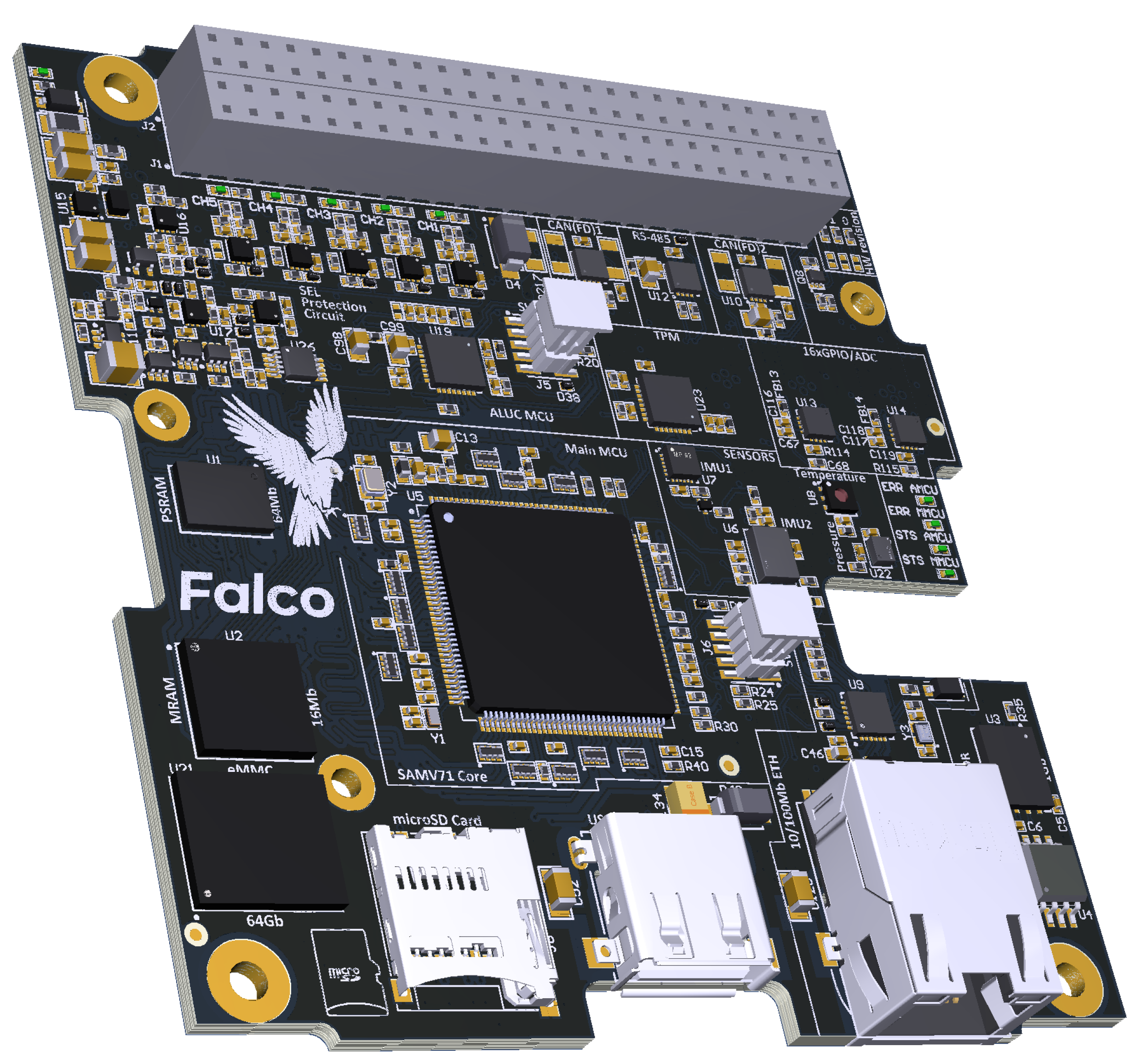
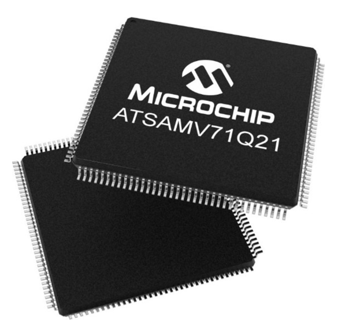
Figure 5.
A ’Boryviter 0.1" microcontroller ATSAMV71Q21
The ’Backup’ mode achieves the lowest possible power consumption. This mode is quite good for applications where recurring and periodic tasks are to be executed, and the microcontroller sleeps the rest of the time. This is a good instrument for low-reliability or slow control systems and does not fit very well with the real-time tasks of the mission control computer. It is important to mention that the core state after return from backup mode is ’reset,’ which means that the specific software design patterns are to be used to construct an appropriate use of this mode.
In our work, we used some effective measurement techniques from [52] to measure time costs for such service operations as interrupt handling and thread-switching delays for virtual machines, which in our article was adapted for a microcontroller and RTOS setup. Given that FreeRTOS operates with the concept of Tasks and the interrupt handling exists within a context of parallel computation, which is largely independent of the scheduler operation, we adopted the mentioned architectural approach to our experiment needs.
3.2. Limitations and Assumptions
The following limitations and assumptions shall apply:
- The supply voltage of the microcontroller is nominal and equal to 3.3 Volts. It is the most reliable supply voltage for the electronics components on the mission computer and allows the best resistance to one-time failures and electromagnetic interference (EMI). There is a power consumption dependence over the supply voltage, but this is not the subject of this research;
- The priorities of the performed tasks are assigned according to the classical theory of Lew and Leyland, called RMS (rate-monotonic scheduling). In this case, each task periodic and characterized by two numbers:where - is the maximum time required for the task execution and is the repetition period of the task.
- A set of N tasks to be performed:is always formed in such a way that they meet the sufficient condition of scheduling tasks of hard real-time systems formulated by Liu and Leyland [26]:
- The limit on the size of the system tick, which determines the frequency of interruptions from the system timer, is obtained from the FreeRTOS documentation, taking into account the limitations of the MPLAB X IDE development environment for the Atmel ATSAMV71 microcontroller:
- The limits on the microcontroller clock frequency are determined based on the technical documentation for the ATSAMV71 microcontroller, hardware clock configuration of the ’Boryviter 0.1’ mission computer and form the following set:
3.3. Experiment Plan
Let’s define the ATSAMV71 microcontroller as a power-state machine with several operating modes: an active mode enabling software to make its main calculations and low-power modes turning off CPU peripherals and components (Figure 6). Dependencies on the clock frequency over the electrical power consumed by the microcontroller in possible power states and the time spent on transitions between them must be obtained based on the results of experiments. Such experiments are conducted in more detail in this article.
Let us divide all the necessary experimental dependencies and structure them into three classes:
- The dependence of energy consumption on frequency. Dependencies of the consumed electric power on the processor clock frequency N(f) must be determined for each operating mode m. The set of possible modes includes the active mode and power saving modes:
-
Time spent by the operating system to perform functions related to rescheduling and dispatching tasks. These events could originate from forced software requests for rescheduling, system timer interrupts due to the next system tick, or external unplanned interrupt triggering OS synchronization facility – Mutexes, Semaphores, Event Groups, and Queues. Here are the definitions of the events identified for the experiment:
- (a)
- Forced software re-scheduling. The FreeRTOS taskYIELD() function is the basic function of cooperative dispatching. It immediately causes rescheduling, forcing the scheduler to check if another task is ready for execution. If such a task exists and has a higher or equal priority than the current one, a context switch to this task will be performed. Unlike external or system tick interrupts, taskYIELD() does not rely on hardware interrupts. Instead, it is a software mechanism in which the running task voluntarily yields execution, allowing other tasks to run. As a result, the taskYIELD() function represents a cooperative approach to multitasking, where tasks manage their own execution time, while external interrupts and system tick interrupts are part of a preemptive system where the OS can forcefully manage task execution based on real-time events and regular scheduling needs. The time required to perform the function is denoted by: ;
- (b)
- System timer interrupt. The processor time spent processing interruptions from the system timer depends on the clock frequency of the computing platform. It characterizes the operating system’s overhead for working in the preemptive multitasking mode. System tick interrupts occur regularly, triggering the OS to perform tasks such as updating the system time, managing the scheduling process, and potentially preempting the current task if necessary. The time required to perform the function is denoted by: ;
- (c)
- External or peripheral interrupt. The time of the system and call of the interrupt service routine (ISR) is the time from the moment of the occurrence of the external or peripheral interrupt to the time of execution of the first command of the interrupt handler. The time required to perform the function is indicated by . When an external interrupt occurs, the Interrupt Service Routine (ISR) handler or the first-level interrupt handler (FLIH) is triggered immediately. This mechanism forces the OS to temporarily stop the current process, handle the interrupt, and then return to the interrupted task or switch to a different task based on priority. It is important to mention that freeRTOS is a very low-footprint RTOS, and in reality, the context of the ISR handler and the rest of the RTOS context are not very closely coupled. In other words, the IRQ handling is like a regular blocking function with an asynchronous call and a primitive calculation context preservation that heavily leans on ARM Cortex M core capabilities.
-
The time spent entering and leaving the low power mode (LPM): The time required to enter and leave a low-power mode will define how much energy can be saved and how bad system reactivity will be decreased. According to the power state-machine definition, two transitions shall be assessed:
- (a)
- Entering. As entering a LPM requires a specific amount of instructions - its time shall be properly measured. Only specific processor peripherals shall be shut off depending on the exact LPM. No memory preservation actions are required.
- (b)
- Leaving. The exit from an LPM requires more sophisticated actions. As some of the LPM modes shut off the internal frequency generator or switch it to the low-power one, a specific stabilization time is required before any processor instruction can be executed.
Thus, the independent factors of the experiment are the clock frequency and the operating mode, and the data that shall be obtained via the experiment are energy consumption, processor time spent on interrupt processing from the system timer, and the delay in the execution of the first instruction of the interrupt processing procedure. A complete factor experiment is planned, in which the factors take the following values:
3.4. Measurement Technique
Typically, all power-saving measurements in modern microcontrollers require quite a comprehensive setup, as they require precise energy measurement, synchronized time-slice measurements, and an external disturbance generator.
For our experiments, the research bench (Figure 7, Figure 8, Figure 9 and Figure 10) was built with the following equipment:
- the square wave generator - GW Instek GFG-8219A that generates external interrupt signals with a given period;
- the high-precision power supply unit and power meter - Keithley 2281S-20-6 that measures the electric energy consumed. It guarantees the accuracy of the measurements (the measurement error of the time interval is no worse than 15 ms, and the error of the electric power measurement does not exceed 0.0001 W;
- the multi-channel storage oscilloscope - LeCroy WavePro 7200A provides the measurement of the time interval between two events: an externally generated interrupt signal from a square wave generator and the first command of the interrupt handler, which is a change of the state of a predefined port - Port 1, to the opposite. Since the command to change the port is atomic, that is, it is executed in one computing cycle in the RISC architecture, the time to change the state of the port can be considered insignificant;
- A hand-modified ’Boryviter 0.1’ mission computer where the oscilloscope is connected to the two GPIO outputs (via flying wires) and to the signal generator.
We had to design a more complicated measurement connection diagram for the second part of the measurements, entering the low-power modes. The key idea was to use the already soldered on a mission computer shunt resistor and operational amplifier to ensure that the proper scale and linearity of the current consumption are captured on the oscilloscope. So the connection diagram for the second test bench includes:
- The high-precision power supply unit and power meter - Keithley 2281S-20-6 was used to measure the electric power consumed;
- A multi-channel oscilloscope – Siglent SDS1204X-E measures the trigger event between the processor command “go to the low-power mode” and the current consumption response of the microcontroller;
- A modified ’Boryviter 0.1’ mission computer where the oscilloscope is connected to the output of the power-monitor operational amplifier, to ensure proper signal linearity and low noise.
The following connection diagrams were designed:
For the three classes of the dependencies defined above, the following measurement technique was used:
- To obtain dependencies of energy consumption on the frequency in the available modes of operation of the microcontroller in the stationary mode of operation, it is enough to set one of the four operating modes (Active, Sleep, Wait, and Backup) and record the electric power consumption by the Keithley 2281S-20-6 power measurement unit;
-
Time spent by the operating system to perform functions related to the rescheduling and dispatching tasks is measured as follows:To estimate the pre-emptive dispatching time, we measured the execution time of the simple pre-defined calculation algorithm with the known execution time for each CPU frequency. For reliable results, a set of 1000 measurements were executed. It is expected that due to the overhead required for handling external interrupts and interrupts from the system timer, some iterations of the known algorithm will take longer. Suppose that the frequency of the external interrupt differs by one and a half to two times from the frequency of the system timer, and the execution time of one iteration is 20-30 percent of the value of the system tick. In that case, we will get the following dependence of the execution time on the iteration number (Figure 11). If the frequencies of interruptions (external and from the system timer) differ by 1.5-2 times, then it is very easy to distinguish their influence on the general graph: it is enough to count the number of measurements that got on the corresponding shelves.The results of measurements of the actual execution time of each iteration are distributed on four shelves, depending on whether the cycle was interrupted for processing interruptions. These shelves correspond to the following situations:
- there are no interruptions;
- an interrupt from the system timer occurred;
- an external interrupt occurred;
- the iteration was interrupted twice by the system timer and externally.
The following algorithm was performed for each CPU frequency to estimate the cooperative dispatch time.The program first accumulates an array of data about the execution time of the mutex ’take’ operation. The FreeRTOS is configured to have only one single task, which blocks and releases the mutex, and then records the time required to perform these two operations in the array.In the second stage, several tasks are created, which block the mutex in a loop, record the time and task number in the logEntries shared array, release the mutex, and then call system function taskYIELD() to transfer control to other tasks. These tasks work in parallel, creating conditions for estimating the overhead of switching between tasks. A hardware timer measures the time of operations with a resolution equal to 66,66 ns. The logEntries array stores the execution time of the operations and the task number, which enables the analysis of the results after the program is executed.Conditional Transition between Stages: The second stage begins after completing the first one, ensuring the correctness of the accumulated data. -
The time spent entering and leaving low-power modes (LPM). According to the processor datasheet, the ’Wait’, ’Sleep’, and ’Backup’ modes require a specific microcontroller shutdown technique that, in return, requires a waiting loop to ensure that all peripherals are safely turned off. However, the ’Backup’ mode, as the most ’deep’ power saving mode, can be exited only if a processor resets. To measure it, it is necessary to apply external devices because when the processor is turned off, and the peripheral shut-off process has been initiated, it is impossible to get information on when exactly the core has stopped working. The time for the transitions [1], [3], [5] in Figure 6 can only be determined using an external oscilloscope since the program is not executed in energy-saving modes. In this case, the actual time of entering the low-power modes can be assessed by the drop in the supply current consumption and, thus, registered with the oscilloscope:
- Step 1. The test software toggles the output GPIO port state. This allows to trigger the connected oscilloscope;
- Step 2. Based on the triggered event of entering the LPM, the second channel of the connected oscilloscope, which is connected to the operational amplifier, registers the current consumption drop;
- Step 3. By calculating the time difference between the triggered event in Step 1 and the current drop event in Step 2, the time required to enter an LPM is obtained.
The exit time measurement technique for the transitions [2], [4], [6] in Figure 6 is also rather hard to do. Still, with the essence of having an external interrupt wake the processor up, it is pretty straightforward to measure the time difference between the external interrupt signal from the signal generator and the output pin toggle of the microcontroller.However, as the most ’deep’ power saving mode, the’ Backup’ mode can be exited only during a processor reset. For this specific case, the test software was modified so that the specific pin toggle was the first operation from the start of the software. The exit from the LPM heavily depends on the particular LPM and how it implements the microcontroller peripheral shutdowns. If the Sleep and Wait modes are relatively straightforward to measure, as both allow them to return to the ’before the LPM’ computation context, the Backup mode is more nontrivial. The exit from the Backup mode requires a RESET vector entrance, which means that the microcontroller software starts from scratch. This behavior requires a more complex software architecture for implementation and typically requires an external NVRAM that could be used as context memory.So, we used two different test software scenarios to measure exit from LPM modes. For both scenarios, the external interrupt from the signal generator was used. That signal triggers the connected oscilloscope to capture the GPIO pin toggle as the first operation after the microcontroller is ready to execute the next command on the program counter (PC).-
Scenario 1 – Sleep and Wait modes:
- -
- Step 1. The wakeup source is configured to react on the external interrupt from the GPIO pin connected to the signal generator;
- -
- Step 2. The external signal generator is set to generate 10 Hz square pulses;
- -
- Step 3. The interrupt handler is done in a way that the first thing it does is the appointed GPIO pin toggle;
- -
- Step 4. The time difference between the rising edge of the square pulse from the signal generator and the rising edge at the output GPIO pin could be considered the wakeup time.
-
Scenario 2 - Backup mode:
- -
- Step 1. The wakeup source is configured to react on the external interrupt from the GPIO pin connected to the signal generator;
- -
- Step 2. The external signal generator is set to generate 10 Hz square pulses;
- -
- Step 3. As the microcontroller shall undergo a reset vector, the GPIO pin toggle was done as the very first operation in the main() function, right after the GPIO configuration. As the test software didn’t contain any major variables, the time for initialization of the “.bss” section can be neglected;
- -
- Step 4. The time difference between the rising edge of the square pulse from the signal generator and the rising edge at the output GPIO pin could be considered the wakeup time.
4. Results
4.1. The Dependence of Energy Consumption on the Operating Frequency
The platform’s power consumption depends linearly on the frequency at a fixed supply voltage (Figure 12). The constant, independent of the frequency of the processor energy consumption, is approximately 130 mW. The slope coefficients of the linear dependencies of the energy consumption on the frequency are shown in the figure. Using the low-power modes of the processor saves up to 60% of energy. This advantage is most noticeable when the processor is running at maximum frequency.
4.2. Time Spent by the Operating System to Perform Functions Related to the Rescheduling and Dispatching Tasks
The measurement technique is described in detail in Section 3.3, ’Time spent by the operating system to perform functions related to rescheduling and dispatching tasks.’ The summary Table 2 characterizes the main reactivity indicators of the operating system on the ’Boryviter 0.1’ platform. In addition to reactivity indicators, the table contains the results of measuring operations with a nonblocking mutex (’take’, ’give’).
Due to the specifics of the ARM Cortex-M computing architecture, which has two independent instruction counters: a full Program Counter (PC) and an "emulated" Link Register (LR), the computer demonstrates sufficiently high reactivity indicators. FreeRTOS effectively supports the ARM Cortex-M architecture, as it does not distinguish between interrupt handling and normal functions. It has been experimentally confirmed that with cooperative dispatching, the execution time of the function taskYield() does not depend on the number of tasks in the system, since the FreeRTOS OS implements the round-robin dispatching mechanism of queued tasks.
4.3. The Time Spent Entering and Leaving the Low Power Modes (LPM)
A typical oscillogram of the decrease in power consumption over time after execution of the command to enter the LPM is shown in Figure 13.
The following Figure 14 illustrates the measurement view of the delay in execution of the first command of the interrupt handler after receiving an external interrupt when the processor was in LPM mode.
Table 3 summarizes the results of the measurements of the integral indicators that characterize the practicality of using LPM modes for energy savings.
There are two main characteristics: wake-up delays characterize the time required for the processor to exit sleep mode fully, and the break-even time is the sum of the wake-up and transition to LPM delays, last characterizes the time required for the processor to transition from the active state to the sleep mode.
5. Discussion
The data presented above confirm the possibility of experimentally determining the following quantitative indicators characterizing the operation of the computing platform under the conditions of time and energy constraints that exist in the on-board avionics of the UAV:
- dependence of power consumption on clock frequency for active mode and low-power modes;
- overhead costs of the operating system to support multitasking, namely delays in the execution of operations of the scheduler and dispatcher of the operating system for the implementation of cooperative and preemptive dispatching;
- break-even and wake-up times when using low-power modes.
Practical application We will discuss the possibility of practical application of the results obtained. We consider the scenario when at the stage of designing both hardware and software of a mission computer of the UAV, there is the following need:
- to ensure that it is functioning energy-efficiently, i.e., spending only a minimum of electrical energy on its operation;
- to guarantee that the required amount of computational work will be completed within the established time frame;
- to ensure that the reaction time to external events will not exceed the established and required by the end-application (mission) limits.
Then, in the list of possible design solutions, one or both of the following must be selected:
- set the clock frequency of the processor, which will be sufficient to guarantee the specified limits;
- apply a software solution to enable one of the existing low-power modes.
Of course, the use of software algorithms to manage power-saving modes has undoubted advantages in terms of flexibility. Still, the possibility of determining the processor’s clock frequency is sufficient for practical use and should not be neglected.
We will not consider the ’Backup’ mode, as it requires a complete processor restart and is characterized by sufficiently large payback time requirements and a completely different software architecture to be applied.
Algorithms to design The results obtained make it possible to design algorithms and energy-saving mechanisms for the mission computer as a solution to the optimization problem. The optimization criterion is the minimum power consumption of the mission computer in various power-saving modes:
where is the relative cost of processor time sufficient to ensure real-time constraints;
- energy consumption for the operation of the mission computer when applying the following approaches to energy saving: low-frequency mode (LF), software-defined transitions to ’Sleep’ and ’Wait’ modes with a return to active mode upon external/internal interruption.
Then, when using each of the low-power modes, the average power consumption will not be greater than during the continuous operation of the processor at the maximum frequency. The relative part of the energy savings for the three modes of energy savings depends on the processor load factor - and, in the case of an ideal mission computer, is calculated as .
The linear dependencies of the consumed electric power for the real computer modes on the frequency can be summarized in the form of an equation:
where the m modes take the following values: , and result as the following:
from the subsection 4.1 (see Figure 11).
So how much energy can we save? The relative part of the energy saved can be calculated for a real computer using the following equations.
Figure 15 illustrates the results of calculating energy savings using energy-saving modes. Limiting the processor’s clock frequency at the design stage is the most beneficial if the system has excessive computing power. Flexible software-controlled methods for switching between ’Sleep’ and ’Wait’ modes do not provide such benefits. However, they have the key advantage of adapting to a specific situation onboard. Estimates of the reactivity of the system in different modes of operation and operating system overheads for multitasking support obtained in the article make it possible to consider overheads for operating system operations.
6. Conclusions
The main goal of this work is to develop and test the technique of experimental search for a compromise between the required reactivity of the real-time system of the mission computer of the UAV and the electrical energy consumption of it.
The technique was approved using the author’s computing platform ’Boryviter 0.1’, which is implemented on the ATSAMV71 microprocessor and operates under the control of the open operating system FreeRTOS. The platform is intended to be used in a dual-purpose UAV and nanosatellites of the CubeSat class. This technique is based on the system model. The system model is a power-state machine that comprehensively characterizes the relationship between energy consumption and reactivity. Next, we define three types of models that are needed to fill this system model. This depends on the clock frequency:
- consumed electrical energy in the active mode and power-saving modes of the on-board computer;
- time spent by the operating system to perform functions related to rescheduling and dispatching tasks. We have considered all three possible cases when the OS performs rescheduling and dispatching: cooperative dispatching, crowding out dispatching after an interrupt from the system timer, and external interrupts;
- time spent on entering the energy-saving mode and returning to the active mode after an external event (interruption) that requires the system to wake up.
Then we determined the measurement techniques to obtain the dependencies mentioned above.
As the work results, a generalization of the experimental results is presented, and quantitative estimates of the measured characteristics for the author’s computing platform ’Boryviter 0.1’ are provided.
We consider the following to be the scientific novelty of the work:
- The task of finding compromises between reactivity and power consumption of the on-board computer is formulated through a representation in the form of a system model - power state machine;
- The developed technique for measuring the time spent pushing dispatching after an interruption from the system timer and processing an external interruption allows you to quickly and accurately determine these costs;
- The proposed time measurement technique for cooperative dispatching is also fast and accurate; besides, it is well-scalable, as it allows us to figure out the system’s behavior with an arbitrary number of tasks.
As a practical result, the article substantiates the conclusion that using a real-time operating system (FreeRTOS) in the author’s computing platform, ’Boryviter 0.1’, fully meets the task of quickly adapting the computing context to changing external factors (like interrupt-driven UAV avionics signals) and the required volume of calculations.
A limitation of our work is a certain idealization of measurement modes when the influence of external factors was considered separately. For practical application, it is necessary to check the adequacy of the obtained mathematical dependencies in the case of a more realistic picture of the existence of many practical tasks inherent in a typical set of calculations when using UAVs. Such practical and real-time deviations could be connected both with the avionics faults, external signals arrival frequency, etc.
In addition to checking the adequacy of the mathematical models obtained, we plan to investigate the reactivity and energy consumption of our computing platform if the component-oriented framework F´ (F Prime) from NASA is used for the development of onboard software. We plan to use it to allow us to quickly develop and deploy the UAV and satellite mission computer software. Potentially, it can also be used for the software of other parts of the avionics. This framework has a relatively high entry threshold. However, it provides mechanisms for component-oriented development available in open access for reuse, facilitating the solution of common tasks.
Author Contributions
“Conceptualization, Oleksandr Liubimov, and Ihor Turkin; methodology, Oleksandr Liubimov; software, Oleksandr Liubimov; validation, Lina Volobuieva, Oleksandr Liubimov; formal analysis, Oleksandr Liubimov, and Valeriy Cheranovskiy; investigation, Oleksandr Liubimov; resources, Lina Volobuieva; data curation, Ihor Turkin; writing—original draft preparation, Lina Volobuieva; writing—review and editing, Oleksandr Liubimov, Ihor Turkin; visualization, Lina Volobuieva; supervision, Ihor Turkin, and Valeriy Cheranovskiy.; All authors have read and agreed to the published version of the manuscript.”
Funding
This research is carried out in the frame and on budget of the national Ukrainian grant project NRFU.2023.04/0143 - “Experimental development and validation of the on-board computer of a dual-purpose unmanned aerial vehicle”
Data Availability Statement
All archived datasets analyzed, and generated during the study, as well as the source code for the experiments can be obtained upon request.
Acknowledgments
Authors acknowledge the help of engineering company EKTOS-UKRAINE LLC for the support in borrowing hardware platforms and helping with the setup and fine-tuning of the toolchain. Visit https://ektos.net/ for more details.
Conflicts of Interest
’The authors declare no conflict of interest.’
References
- Mueller, M.M.; Dietenberger, S.; Nestler, M.; Hese, S.; Ziemer, J.; Bachmann, F.; Leiber, J.; Dubois, C.; Thiel, C. Novel UAV Flight Designs for Accuracy Optimization of Structure from Motion Data Products. Remote Sensing 2023, 15. [Google Scholar] [CrossRef]
- IAMD Centre of Excellence. The Evolving UAS Threat: Lessons from the Russian-Ukrainian War Since 2022 on Future Air Defence Challenges and Requirements, 2024. Last accessed 8 September 2024, https://iamd-coe.org/wp-content/uploads/2024/02/The-Evolving-UAS-Threat-Lessons-from-the-Russian-Ukrainian-War-Since-2022-on-Future-Air-Defence-Challenges-and-Requirements.pdf.
- Rabiu, L.; Ahmad, A.; Gohari, A. Advancements of Unmanned Aerial Vehicle Technology in the Realm of Applied Sciences and Engineering A Review. Journal of Advanced Research in Applied Sciences and Engineering Technology 2024, 40, 74–95. [Google Scholar] [CrossRef]
- Telli, K.; Kraa, O.; Himeur, Y.; Ouamane, A.; Boumehraz, M.; Atalla, S.; Mansoor, W. A Comprehensive Review of Recent Research Trends on Unmanned Aerial Vehicles (UAVs). Systems 2023, 11. [Google Scholar] [CrossRef]
- Aabid, A.; Parveez, B.; Parveen, N.; Khan, S.; Raheman, M.A.; Zayan, M.; Ahmed, O. Reviews on Design and Development of Unmanned Aerial Vehicle (Drone) for Different Applications. Journal of Mechanical Engineering Research and Developments 2022, 45, 53–69. [Google Scholar]
- Fortune.com. Unmanned Systems / Unmanned Aerial Vehicle (UAV) Market, 2024. Last accessed 28 August 2024, https://www.fortunebusinessinsights.com/industry-reports/unmanned-aerial-vehicle-uav-market-101603.
- Owaid, S.; Miry, A.; Salman, T. Survey on UAV Communications: Systems, Communication Technologies, Networks, Application. University of Thi-Qar Journal for Engineering Sciences 2023, 13, 136–145. [Google Scholar] [CrossRef]
- Jiang, Y.; Xu, X.X.; Zheng, M.Y.; Zhan, Z.H. Evolutionary computation for unmanned aerial vehicle path planning: a survey. Artificial Intelligence Review 2024, 57. [Google Scholar] [CrossRef]
- Ahmed, F.; Jenihhin, M. A Survey on UAV Computing Platforms: A Hardware Reliability Perspective. Sensors 2022, 22, 6286. [Google Scholar] [CrossRef]
- Kumar, P.; Manoj, N.; Sudheer, N.; Bhat, P.; Arya, A.; Sharma, R. UAV Swarm Objectives: A Critical Analysis and Comprehensive Review. SN Computer Science 2024, 5. [Google Scholar] [CrossRef]
- Saravanakumar, Y.N.; Sultan, M.T.H.; Shahar, F.S.; Giernacki, W.; Łukaszewicz, A.; Nowakowski, M.; Holovatyy, A.; Stępień, S. Power Sources for Unmanned Aerial Vehicles: A State-of-the Art. Applied Sciences 2023, 13. [Google Scholar] [CrossRef]
- Liubimov, O.; Turkin, I. Optimizing the CubeSat On-Board Computer Power Consumption Under Hard Real-Time Constraints. Integrated Computer Technologies in Mechanical Engineering - 2023; Nechyporuk, M., Pavlikov, V., Krytskyi, D., Eds.; Springer Nature Switzerland: Cham, 2024; pp. 404–414. [Google Scholar]
- Liubimov, O.; Liubimov, M. USE OF OPEN-SOURCE COTS/MOTS HARDWARE AND SOFTWARE PLATFORMS FOR THE BUILD UP OF THE CUBESAT NANOSATELLITES. Journal of Rocket-Space Technology 2023, 31, 138–147. [Google Scholar] [CrossRef]
- Microchip. COTS-to-Radiation-Tolerant and Radiation-Hardened Devices, 2019. Last accessed 28 June 2023, https://www.microchip.com/en-us/solutions/aerospace-and-defense/products/microcontrollers-and-microprocessors/cots-to-radiation-tolerant-and-radiation-hardened-devices.
- Siewert, S.; Rocha, K.; Butcher, T.; Pederson, T. Comparison of Common Instrument Stack Architectures for Small UAS and CubeSats. 2021 IEEE Aerospace Conference (50100), 2021, pp. 1–17. [CrossRef]
- NASA.gov. State-of-the-Art Small Spacecraft Technology: Small Spacecraft Systems Virtual Institute., 2023. Last accessed 28 August 2024, https://www.nasa.gov/smallsat-institute/sst-soa.
- Microchip. ATSAMV71Q21 Microprocessor Page, 2020. Last accessed 28 June 2023, https://www.microchip.com/en-us/product/ATSAMV71Q21.
- Maltezos, E.; Karagiannidis, L.; Douklias, T.; Dadoukis, A.; Amditis, A.; Sdongos, E. Preliminary design of a multipurpose UAV situational awareness platform based on novel computer vision and machine learning techniques. 2020 5th South-East Europe Design Automation, Computer Engineering, Computer Networks and Social Media Conference (SEEDA-CECNSM), 2020, pp. 1–8. [CrossRef]
- Zhao, X.; Zhou, S.; Lei, L.; Deng, Z. Siamese Network for Object Tracking in Aerial Video. 2018 IEEE 3rd International Conference on Image, Vision and Computing (ICIVC), 2018, pp. 519–523. [CrossRef]
- Zhu, P.; Wen, L.; Du, D.; Bian, X.; Fan, H.; Hu, Q.; Ling, H. Detection and Tracking Meet Drones Challenge. IEEE Transactions on Pattern Analysis and Machine Intelligence 2022, 44, 7380–7399. [Google Scholar] [CrossRef] [PubMed]
- Cai, Y.; Zhang, E.; Qi, Y.; Lu, L. A Review of Research on the Application of Deep Reinforcement Learning in Unmanned Aerial Vehicle Resource Allocation and Trajectory Planning. 2022 4th International Conference on Machine Learning, Big Data and Business Intelligence (MLBDBI), 2022, pp. 238–241. [CrossRef]
- Chodnicki, M.; Siemiatkowska, B.; Stecz, W.; Stępień, S. Energy Efficient UAV Flight Control Method in an Environment with Obstacles and Gusts of Wind. Energies 2022, 15. [Google Scholar] [CrossRef]
- Myasischev, A. Creation of a Rotor-Type UAV with Flight Controllers, Based On a ATmega2560 and STM32f405 Microprocessors. International Journal of Emerging Trends & Technology in Computer Science 2020. [Google Scholar] [CrossRef]
- Jr., R.L.B.; Canham, T.K.; Watney, G.J.; Reder, L.J.; Levison, J.W. Jr., R.L.B.; Canham, T.K.; Watney, G.J.; Reder, L.J.; Levison, J.W. F Prime: An Open-Source Framework for Small-Scale Flight Software Systems. Proceedings of SSC-18-XII-04 32nd Annual AIAA/USU Conference on Small Satellites;, 2018; pp. 110–119.
- Liubimov, O.; Turkin, I.; Pavlikov, V.; Volobuyeva, L. Agile Software Development Lifecycle and Containerization Technology for CubeSat Command and Data Handling Module Implementation. Computation 2023, 11. [Google Scholar] [CrossRef]
- Liu, C.L.; Layland, J.W. Scheduling Algorithms for Multiprogramming in a Hard-Real-Time Environment. J. ACM 1973, 20, 46–61. [Google Scholar] [CrossRef]
- Zhang, F.; Burns, A. Schedulability Analysis for Real-Time Systems with EDF Scheduling. IEEE Transactions on Computers 2009, 58, 1250–1258. [Google Scholar] [CrossRef]
- Bernat, G.; Burns, A.; Liamosi, A. Weakly hard real-time systems. IEEE Transactions on Computers 2001, 50, 308–321. [Google Scholar] [CrossRef]
- Choi, H.; Kim, H.; Zhu, Q. Job-Class-Level Fixed Priority Scheduling of Weakly-Hard Real-Time Systems. 2019 IEEE Real-Time and Embedded Technology and Applications Symposium (RTAS), 2019, pp. 241–253. [CrossRef]
- Shi, J.; Ueter, N.; Chen, J.J.; Chen, K.H. Average Task Execution Time Minimization under (m, k) Soft Error Constraint. 2023 IEEE 29th Real-Time and Embedded Technology and Applications Symposium (RTAS), 2023, pp. 1–13. [CrossRef]
- Adam, G.K. Timing and Performance Metrics for TWR-K70F120M Device. Computers 2023, 12. [Google Scholar] [CrossRef]
- RaspberryPi. RP2040 Microprocessor Page, 2020. Last accessed 28 June 2023, https://www.raspberrypi.com/products/rp2040/.
- Mittal, S. A survey of techniques for improving energy efficiency in embedded computing systems. International Journal of Computer Aided Engineering and Technology 2014, 6, 440–459. [Google Scholar] [CrossRef]
- Widhalm, D.; Goeschka, K.M.; Kastner, W. Undervolting on wireless sensor nodes: a critical perspective. Proceedings of the 23rd International Conference on Distributed Computing and Networking; Association for Computing Machinery: New York, NY, USA, 2022. [Google Scholar] [CrossRef]
- Reghenzani, F.; Guo, Z.; Fornaciari, W. Software Fault Tolerance in Real-Time Systems: Identifying the Future Research Questions. ACM Comput. Surv. 2023, 55. [Google Scholar] [CrossRef]
- Kim, B.; Yang, H. Reliability Optimization of Real-Time Satellite Embedded System Under Temperature Variations. IEEE Access 2020, 8, 224549–224564. [Google Scholar] [CrossRef]
- IEC-61508. IEC 61508 Ed. 2.0 en:2010 CMV, Functional Safety Of Electrical/Electronic/Programmable Electronic Safety-Related Systems - Parts 1 To 7 Together With A Commented Version (See Functional Safety And IEC 61508), 2021. Last accessed 26 Aug 2023, https://webstore.ansi.org/standards/iec/iec61508eden2010cmv.
- ISO-26262. ISO 26262-6:2018, Road vehicles — Functional safety — Part 6: Product development at the software level, 2018. Last accessed 26 Aug 2023, https://www.iso.org/standard/68388.html.
- Zidar, J.; Matic, T.; Aleksi, I.; Hocenski, Z. Dynamic Voltage and Frequency Scaling as a Method for Reducing Energy Consumption in Ultra-Low-Power Embedded Systems. Electronics 2024, 13. [Google Scholar] [CrossRef]
- Oliveira, G.; Lima, G. Scheduling and energy savings for small scale embedded FreeRTOS-based real-time systems. Design Automation for Embedded Systems 2023, 27, 1–27. [Google Scholar] [CrossRef]
- Musaddiq, A.; Zikria, Y.B.; Hahm, O.; Yu, H.; Bashir, A.K.; Kim, S.W. A Survey on Resource Management in IoT Operating Systems. IEEE Access 2018, 6, 8459–8482. [Google Scholar] [CrossRef]
- FreeRTOS.org. Low Power Support: Tickless Idle Mode, 2024. Last accessed 15 August 2024, https://www.freertos.org/Documentation/02-Kernel/02-Kernel-features/07-Lower-power-support.
- Simonovic, M.; Saranovac, L. Power management implementation in FreeRTOS on LM3S3748. Serbian Journal of Electrical Engineering 2013, 10, 199–208. [Google Scholar] [CrossRef]
- Bambagini, M.; Marinoni, M.; Aydin, H.; Buttazzo, G. Energy-Aware Scheduling for Real-Time Systems: A Survey. ACM Trans. Embed. Comput. Syst. 2016, 15. [Google Scholar] [CrossRef]
- de Melo, A.C.C.P.; Café, D.C.; Alves Borges, R. Assessing Power Efficiency and Performance in Nanosatellite Onboard Computer for Control Applications. IEEE Journal on Miniaturization for Air and Space Systems 2020, 1, 110–116. [Google Scholar] [CrossRef]
- Poovey, J.A.; Conte, T.M.; Levy, M.; Gal-On, S. A Benchmark Characterization of the EEMBC Benchmark Suite. IEEE Micro 2009, 29, 18–29. [Google Scholar] [CrossRef]
- Iqbal, S.M.Z.; Liang, Y.; Grahn, H. ParMiBench - An Open-Source Benchmark for Embedded Multiprocessor Systems. IEEE Computer Architecture Letters 2010, 9, 45–48. [Google Scholar] [CrossRef]
- Zoni, D.; Galimberti, A.; Fornaciari, W. A Survey on Run-time Power Monitors at the Edge. ACM Comput. Surv. 2023, 55. [Google Scholar] [CrossRef]
- Kluge, F.; Rochange, C.; Ungerer, T. EMSBench: Benchmark and Testbed for Reactive Real-Time Systems. Leibniz Transactions on Embedded Systems 2017, 4, 02:1–02:23. [Google Scholar] [CrossRef]
- Dobija, K. Countering Unmanned Aerial Systems (UAS) in Military Operations. Safety & Defense 2023, 9, 74–82. [Google Scholar] [CrossRef]
- Liubimov, O. Falco Engineering, 2024. Last accessed 28 Aug 2024, https://www.falco.engineering/.
- Fayyad-Kazan, H.; Perneel, L.; Timmerman, M. Benchmarking the Performance of Microsoft Hyper-V server, VMware ESXi and Xen Hypervisors. Journal of Emerging Trends in Computing and Information Sciences 2013, 4, 922–933. [Google Scholar]
Figure 1.
Global Unmanned UAV Market Share by UAV Class (2022), source: Fortune Business Insights [6]
Figure 1.
Global Unmanned UAV Market Share by UAV Class (2022), source: Fortune Business Insights [6]
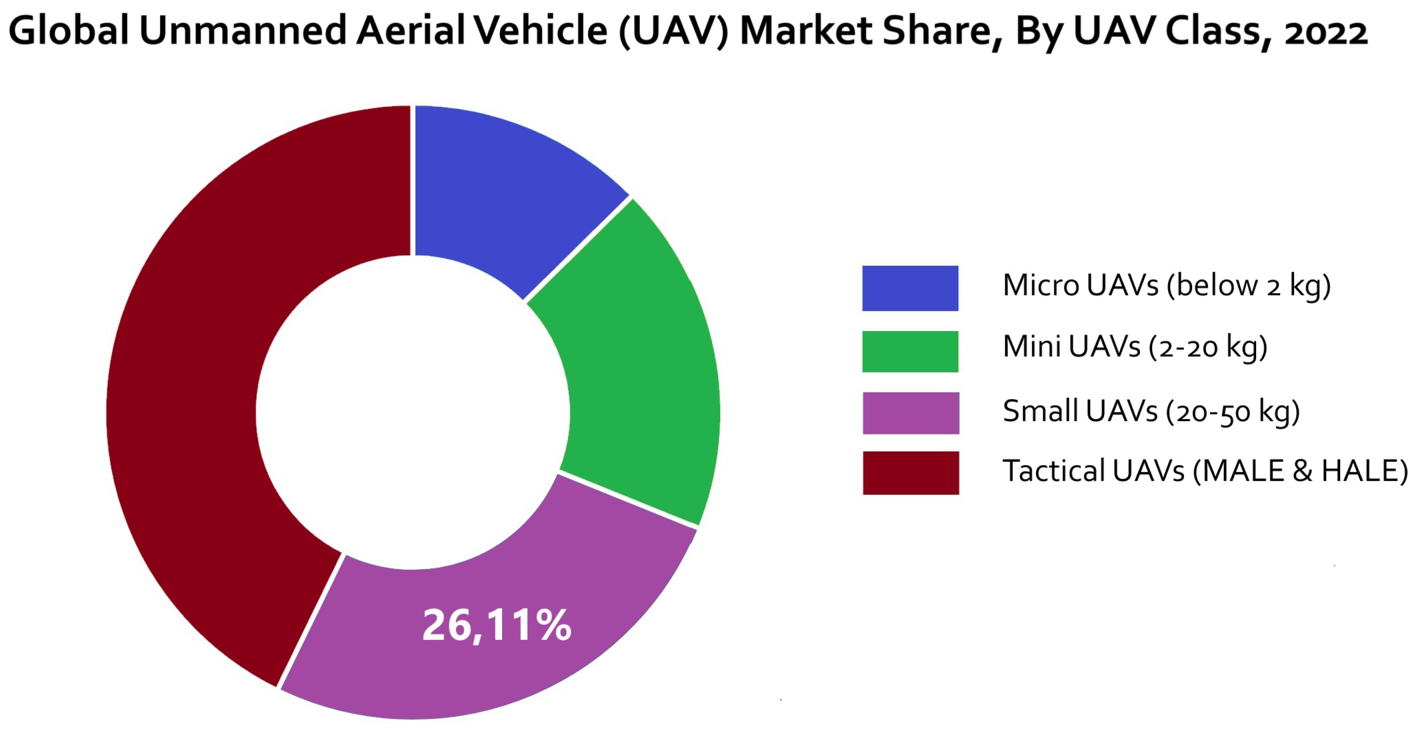
Figure 2.
A typical build-up of the UAV (avionics, batteries, servos, IMUs.
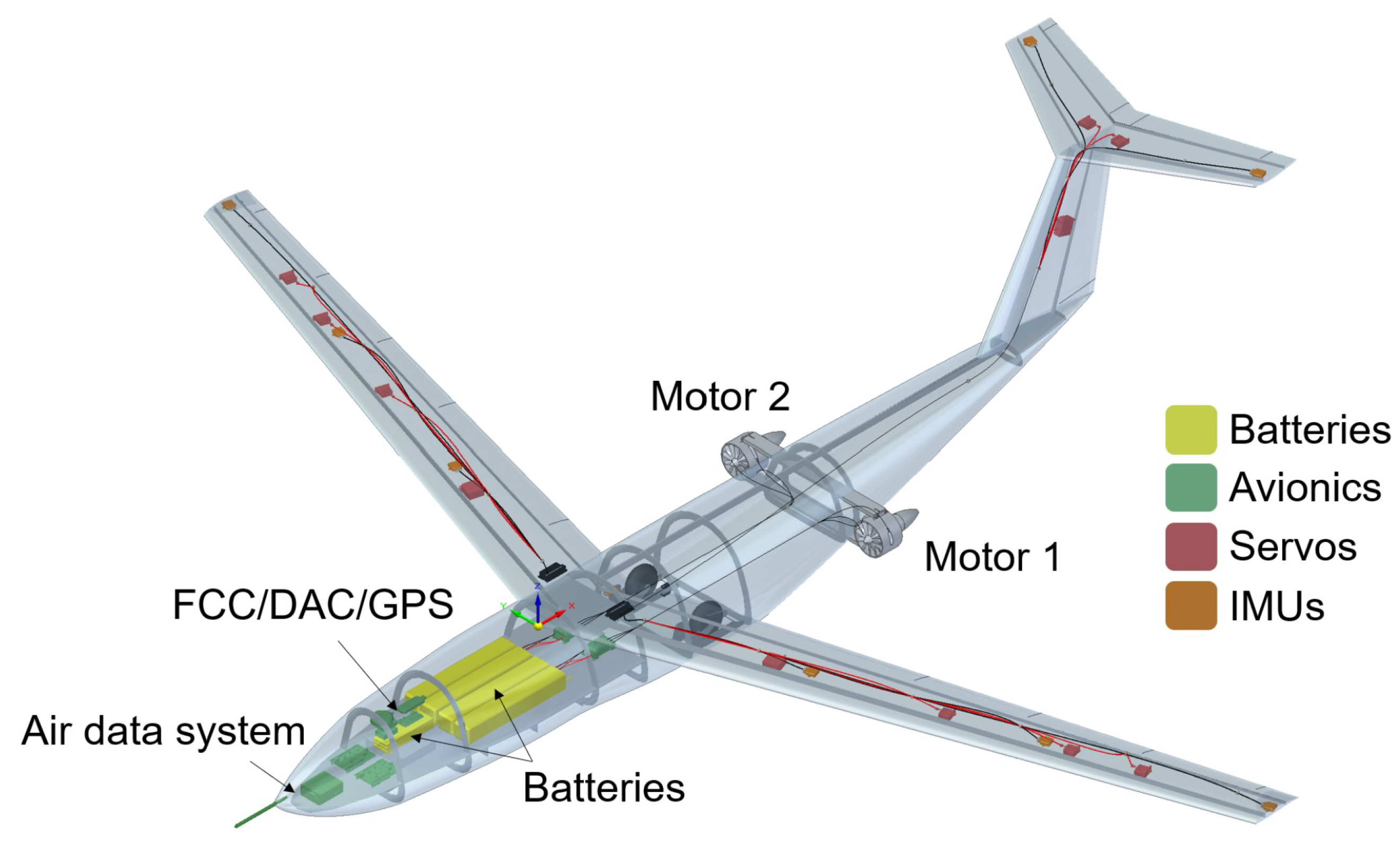
Figure 3.
Typical UAV avionics structure[11]
Figure 3.
Typical UAV avionics structure[11]
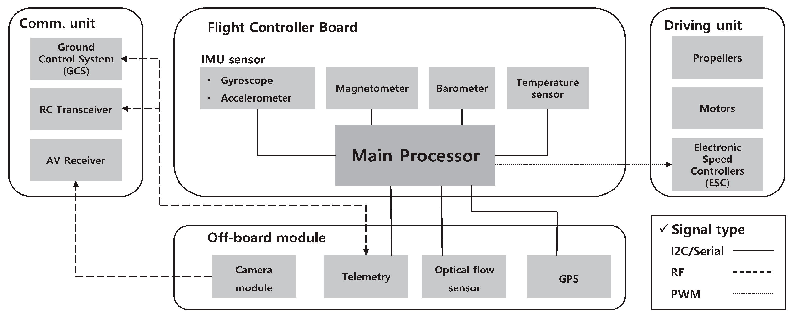
Figure 6.
Power state machine of the ATSAMV71 microcontroller. The initial state is Activemode.
Transitions [1],[3],[5]) characterize the time it takes to enter energy-saving and low-power modes, and
transitions [2],[4],[6] are the time required to restore the active mode after an external interruption
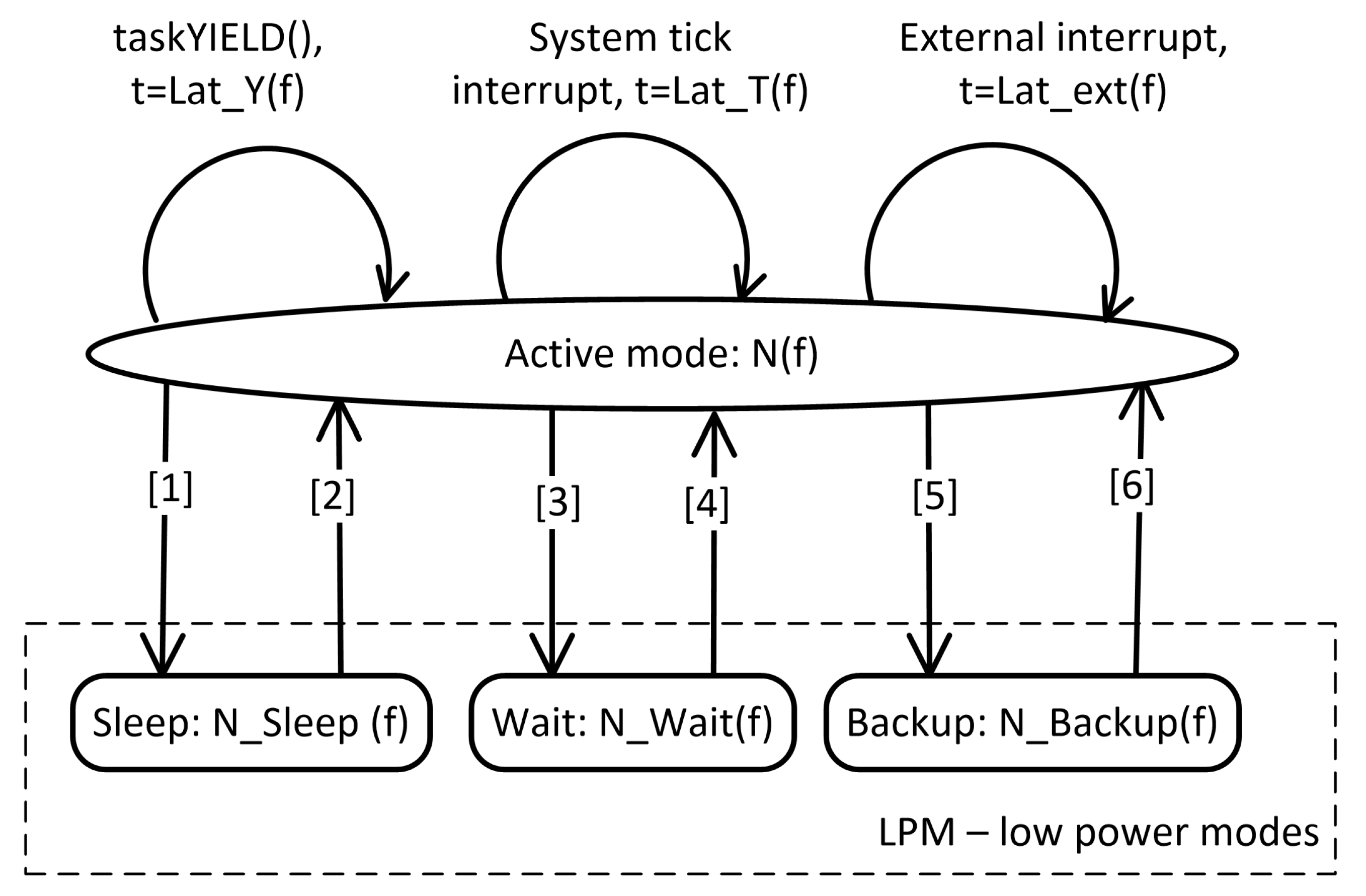
Figure 7.
The connection of mis-
sion computer ’Boryviter 0.1’ (eng.
Falco), to the measurements laptop
Figure 7.
The connection of mis-
sion computer ’Boryviter 0.1’ (eng.
Falco), to the measurements laptop
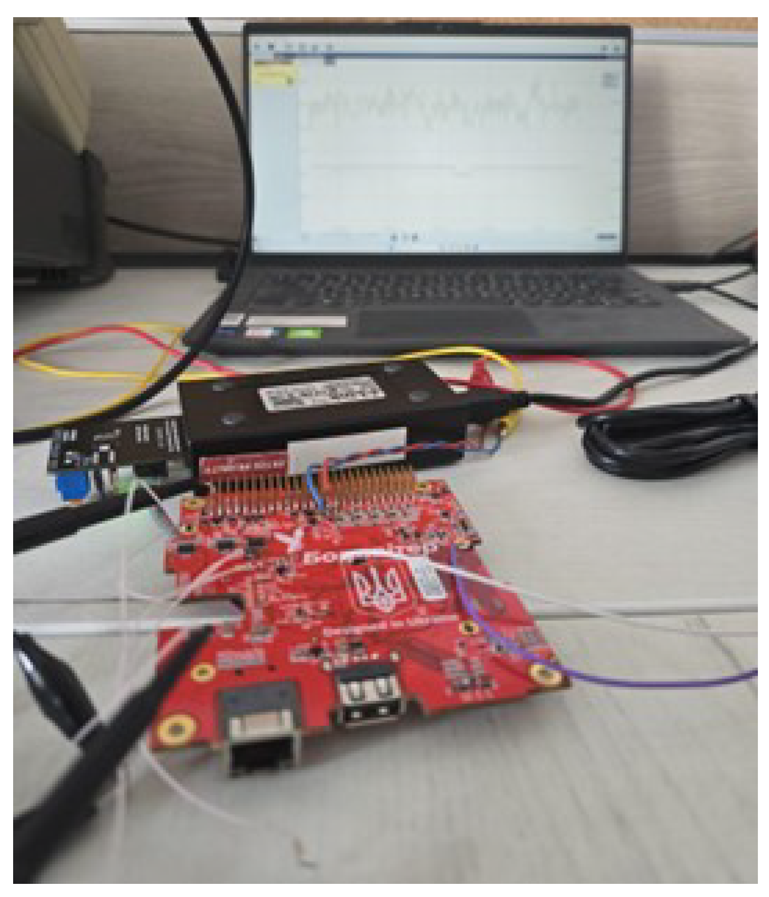
Figure 8.
"Measurement equipment used for the experiment
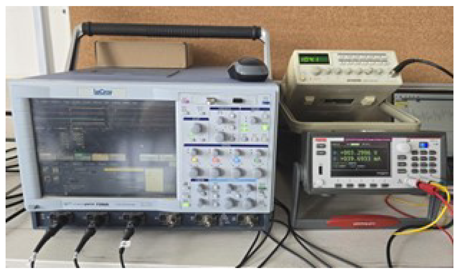
Figure 9.
Test bench connection diagram for time measurements of the transitions [1], [3], [5] from power state machine
Figure 9.
Test bench connection diagram for time measurements of the transitions [1], [3], [5] from power state machine
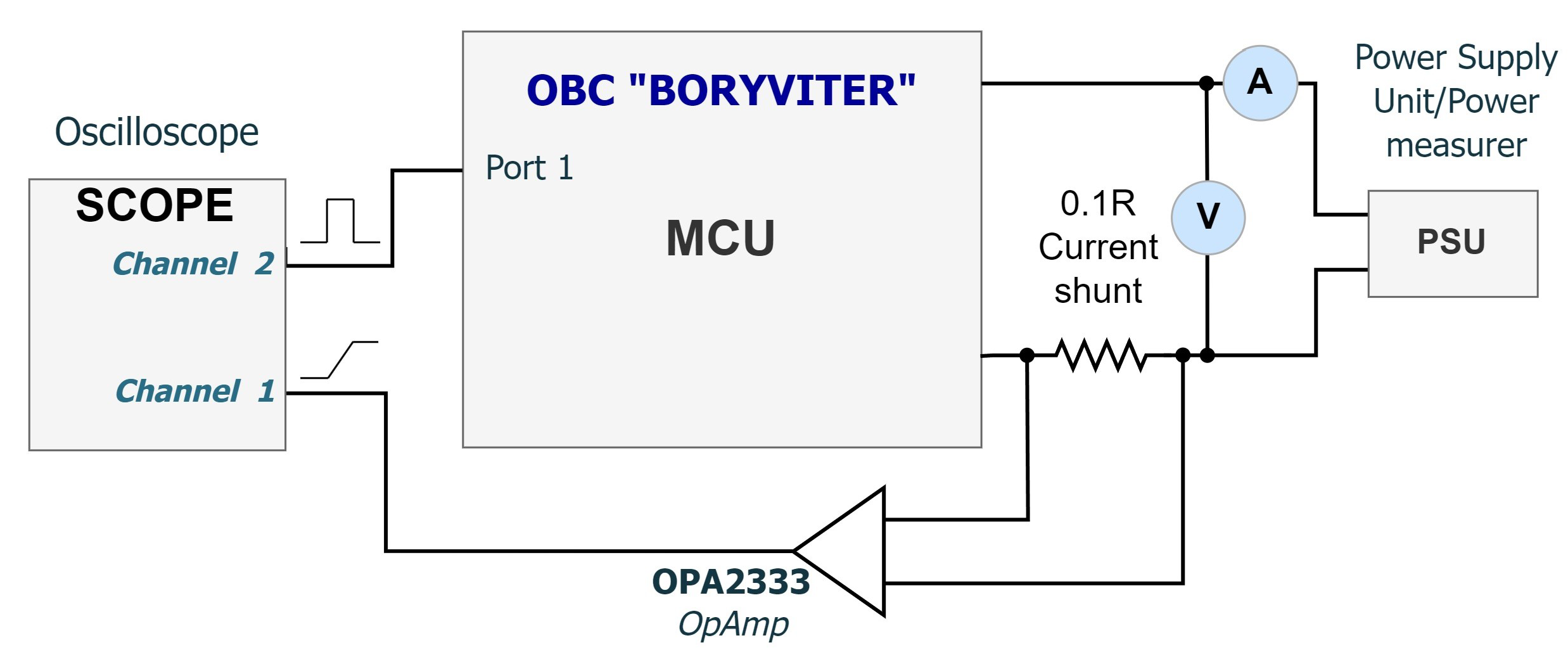
Figure 10.
Test bench connection diagram for time measurements of the transitions [2], [4], [6] from power state machine
Figure 10.
Test bench connection diagram for time measurements of the transitions [2], [4], [6] from power state machine
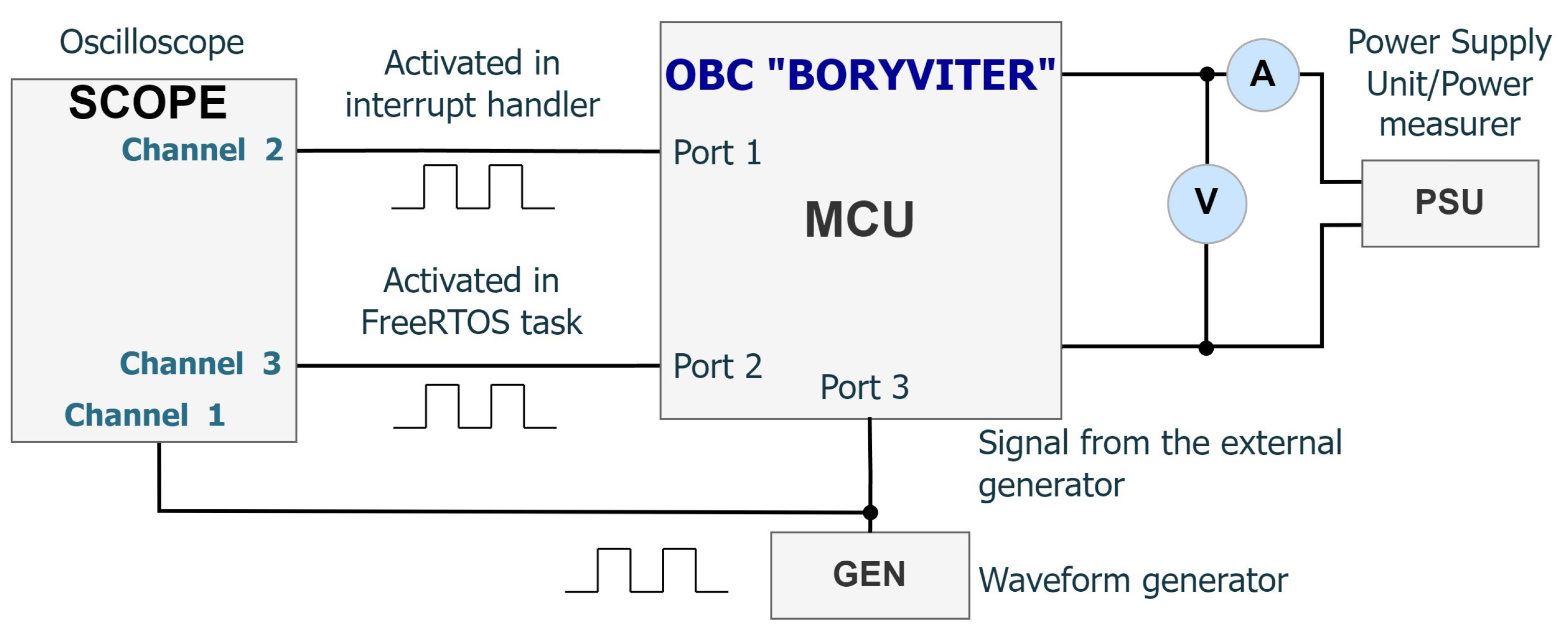
Figure 11.
Example of the obtained dependence of the actual execution time on the iteration number
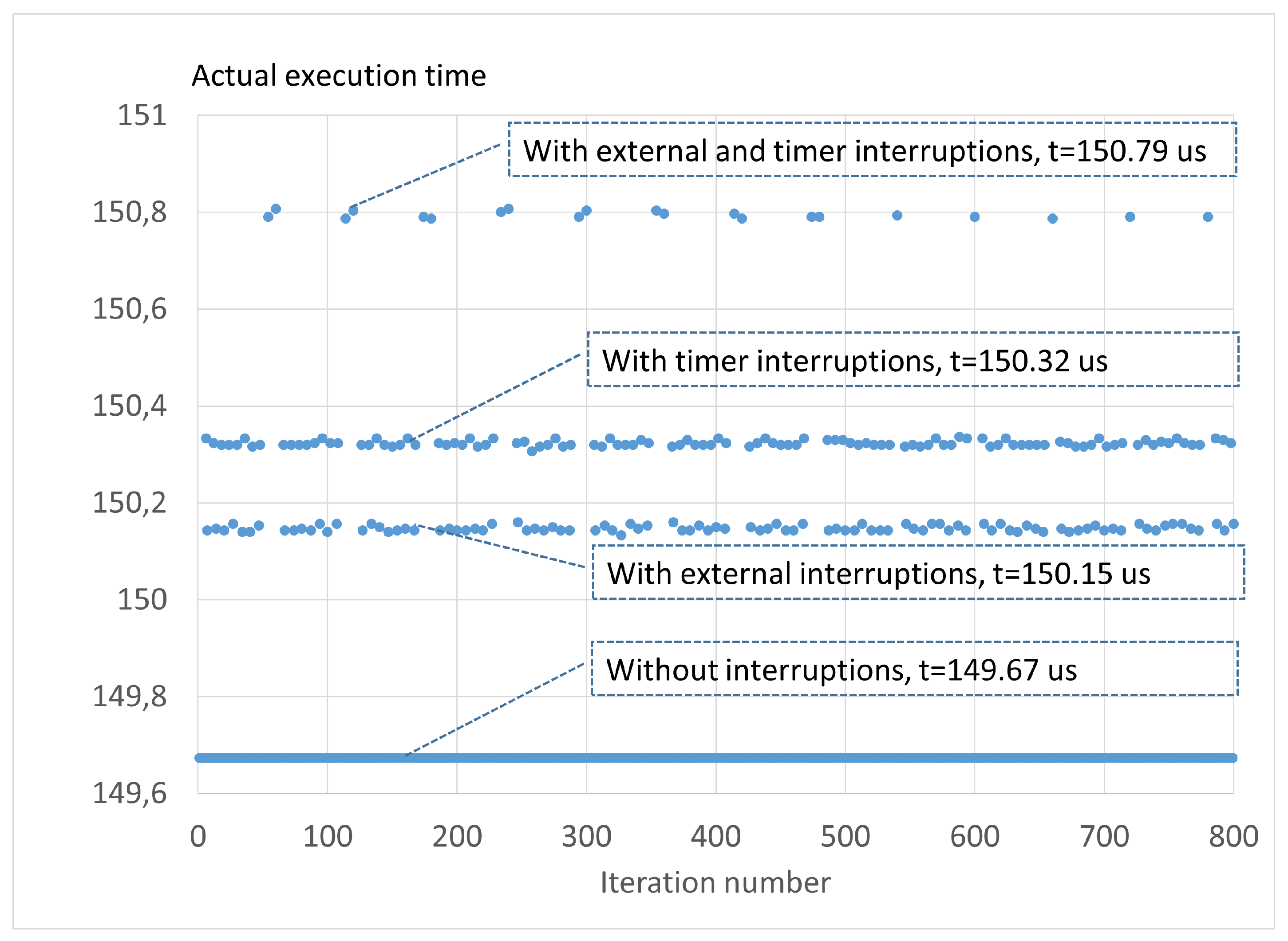
Figure 12.
Dependence of the power consumption of the platform on the frequency in different operating modes of the computer and a fixed supply voltage
Figure 12.
Dependence of the power consumption of the platform on the frequency in different operating modes of the computer and a fixed supply voltage
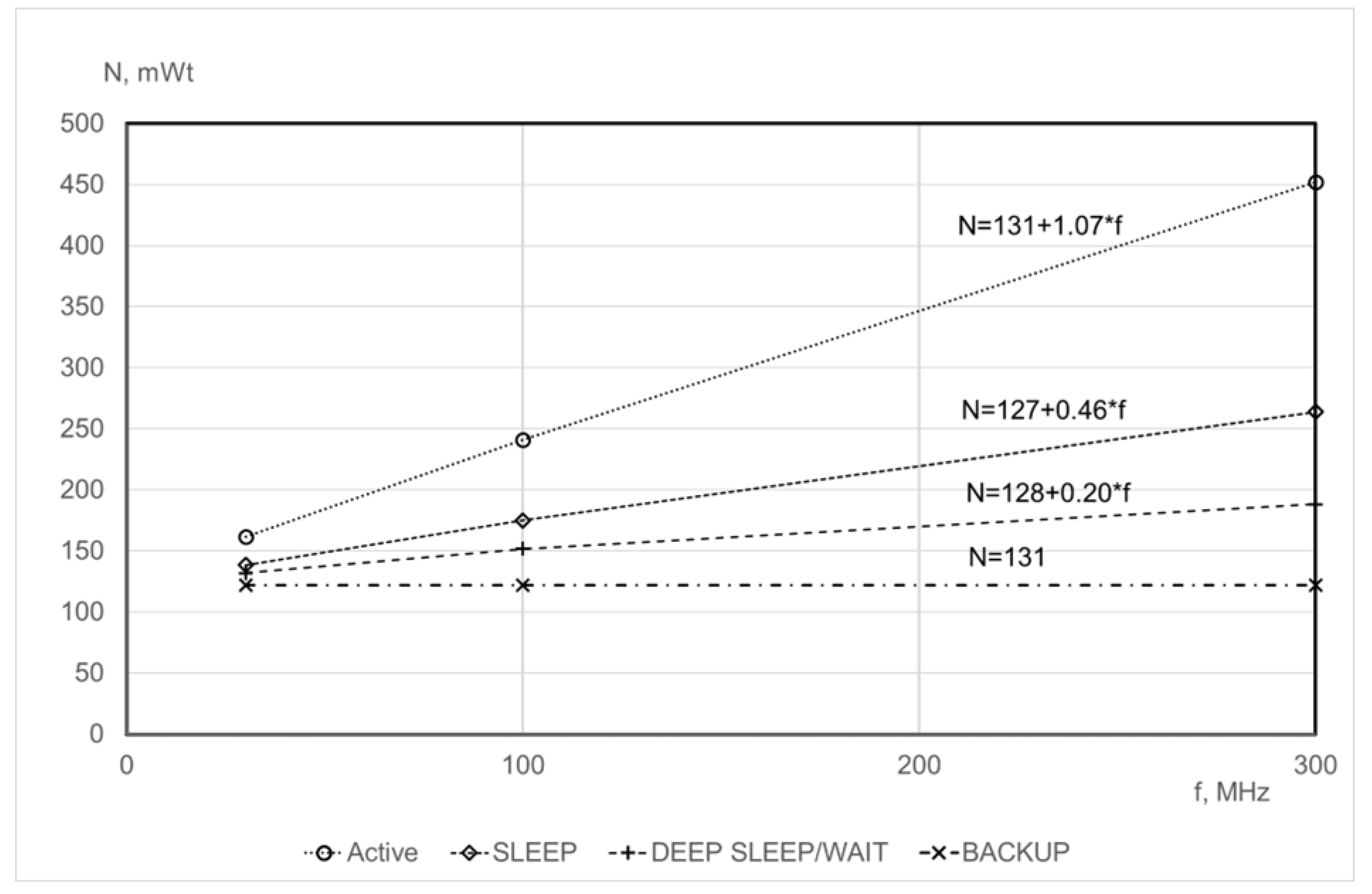
Figure 13.
Entering Wait Mode @ 100 MHz. Current consumption curve. Rough duration = 150±10 uS. C1 (yellow) is a command for entering LPM, and C2 (pink) is the current consumption of the microcontroller.
Figure 13.
Entering Wait Mode @ 100 MHz. Current consumption curve. Rough duration = 150±10 uS. C1 (yellow) is a command for entering LPM, and C2 (pink) is the current consumption of the microcontroller.
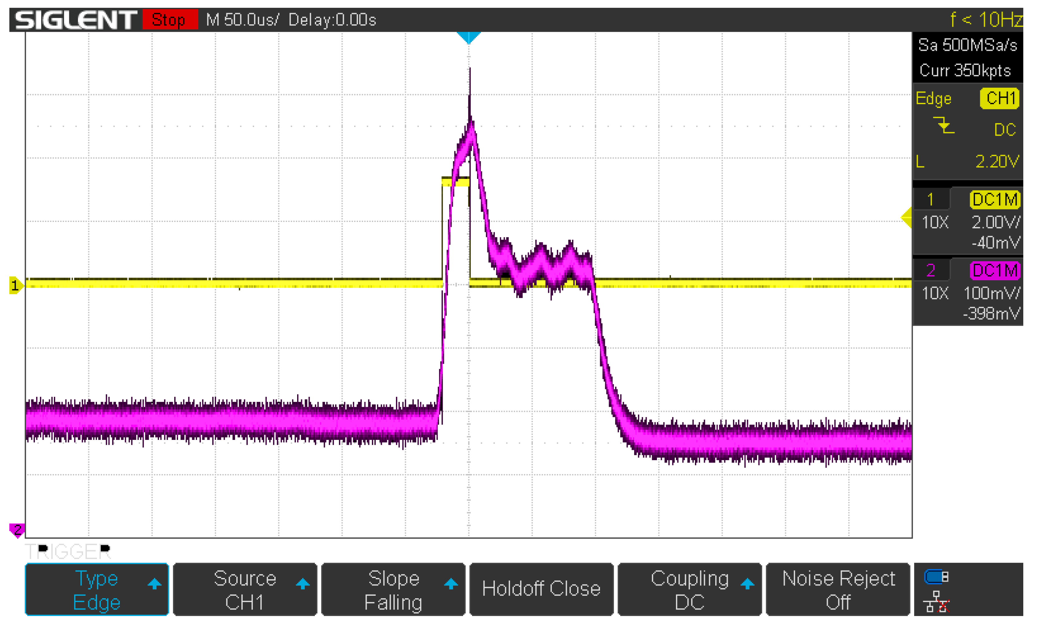
Figure 14.
Leaving LPM timing measurements. Sleep mode @ 30 MHz. C1 – External signal generator pulse, C2 – GPIO pin toggle after wakeup, C3 – the mathematical sum of the time between the rising edges of the corresponding pulses = wakeup time.
Figure 14.
Leaving LPM timing measurements. Sleep mode @ 30 MHz. C1 – External signal generator pulse, C2 – GPIO pin toggle after wakeup, C3 – the mathematical sum of the time between the rising edges of the corresponding pulses = wakeup time.
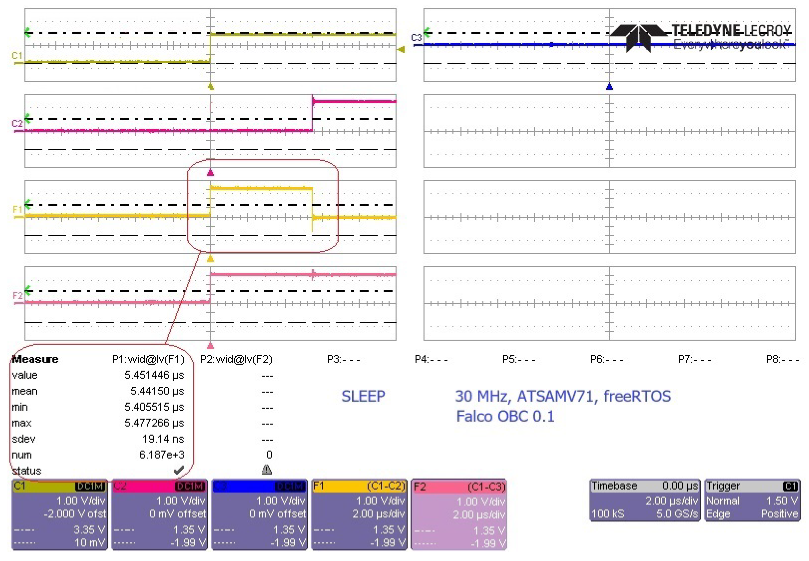
Figure 15.
Optimistic assessment of the possibility of energy saving due to software control of computer operating modes
Figure 15.
Optimistic assessment of the possibility of energy saving due to software control of computer operating modes
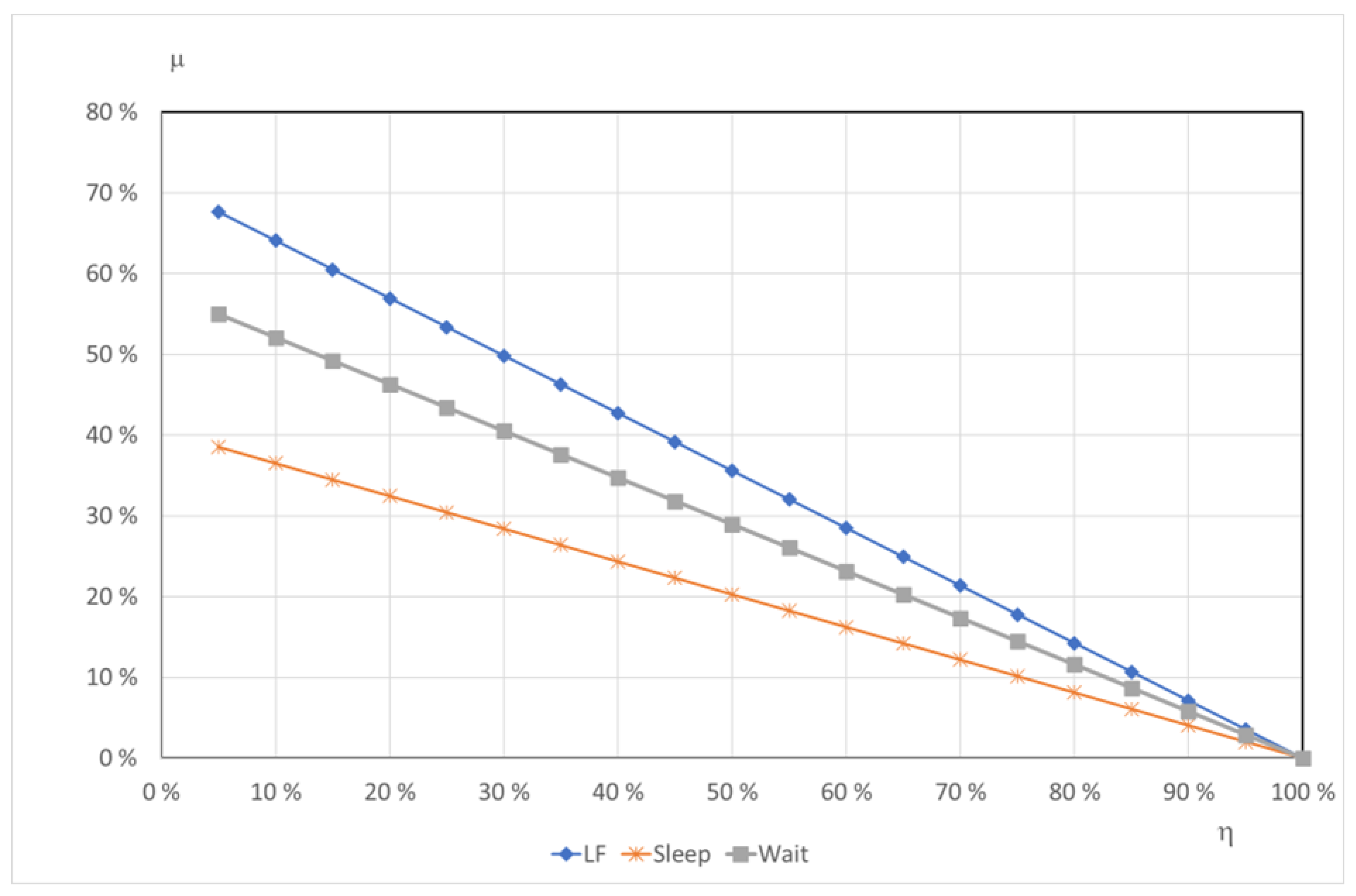

Table 1.
Key characteristics and low power modes (LPM) of a popular series of 32-bit microcontrollers (F - the amount of Flash memory available onboard, R - the amount of RAM available onboard)
Table 1.
Key characteristics and low power modes (LPM) of a popular series of 32-bit microcontrollers (F - the amount of Flash memory available onboard, R - the amount of RAM available onboard)
| MCU Family | Memories | Temperature | Voltage | Low Power Modes |
|---|---|---|---|---|
| ATSAMV7x (Cortex-M7) | F=2Mb, R=384 Kb | -40/+125 | 1.8-3.6 Vdc | Sleep, Wait, Backup |
| PIC32CZ (MIPS) | F=2Mb, R=512 Kb | -40/+105 | 2.5-3.6 Vdc | Sleep, Wait, Backup |
| PIC32MX (MIPS) | F=512Kb, R=128 Kb | -40/+105 | 2.3-3.6 Vdc | Sleep, Idle |
| STM32H7 (Cortex-M7) | F=1Mb, R=564 Kb | -40/+125 | 1.62-3.6 Vdc | Sleep, Stop, Standby |
| STM32F7 (Cortex-M7) | F=2Mb, R=512 Kb | -40/+105 | 1.7-3.6 Vdc | Sleep, Stop, Standby |
| iMX.RT1024 (Cortex-M7) | F=4Mb, R=256 Kb | -40/+105 | 3.0-3.6 Vdc | LPR (24 MHz), Sleep |
Table 2.
The summary table of the time spent by the operating system to perform functions related to the rescheduling and dispatching tasks
Table 2.
The summary table of the time spent by the operating system to perform functions related to the rescheduling and dispatching tasks
| Frequency, MHz | taskYield() latency , uS | System tick interrupt latency , uS | External interrupt latency , uS | Capturing and releasing non-blocking mutexes latency, uS |
|---|---|---|---|---|
| 30 | 7,27 | 4,02 | 6,42 | 7,73 |
| 100 | 2,16 | 1,23 | 1,95 | 2,34 |
| 300 | 0,72 | 0,47 | 0,65 | 0,78 |
Table 3.
The time for wake-up delays and break-even time (uncertainty no more than 10%):
| Mode | Sleep, uS | Wait, uS | Backup, uS | |||
|---|---|---|---|---|---|---|
| Frequency | Wake-up delays | break-even time | Wake-up delays | break-even time | Wake-up delays | break-even time |
| 30 MHz | 5 | 45 | 1800 | 1950 | 5000 | 6500 |
| 100 MHz | 1,7 | 31 | 1228 | 1388 | 5000 | 6500 |
| 300 MHz | 0,6 | 21 | 105 | 255 | 5000 | 6500 |
Disclaimer/Publisher’s Note: The statements, opinions and data contained in all publications are solely those of the individual author(s) and contributor(s) and not of MDPI and/or the editor(s). MDPI and/or the editor(s) disclaim responsibility for any injury to people or property resulting from any ideas, methods, instructions or products referred to in the content. |
© 2024 by the authors. Licensee MDPI, Basel, Switzerland. This article is an open access article distributed under the terms and conditions of the Creative Commons Attribution (CC BY) license (http://creativecommons.org/licenses/by/4.0/).
Copyright: This open access article is published under a Creative Commons CC BY 4.0 license, which permit the free download, distribution, and reuse, provided that the author and preprint are cited in any reuse.


