Submitted:
24 October 2024
Posted:
25 October 2024
You are already at the latest version
Abstract
This work is a physical review, with elements of additions and thinning, on the methods of theoretical studies of nonlinear electrophysical phenomena in crystals with ion-molecular chemical bonds (CIMB). Crystals of this class include ionic dielectrics (characterized by high ionic conductivity), layered crystals, a special case of which are hydrogen-bonded crystals (HBC), defined as proton semiconductors and dielectrics (PSD).A scientific review (comparative analysis and justification of various approximations) was carried out on the methods of constructing and solving a generalized quasi-classical kinetic equation describing the mechanism of nonlinear relaxation polarization and conductivity processes in dielectric materials with ion-molecular chemical bonds (a special case is hydrogen-bonded crystals (HBC)) in a wide temperature range (1-1550 K) and polarizing field strengths (0.1-1000 V/m) at alternating field frequencies of the order of 1 kHz - 1000 MHz. The most important variant of the equations of the kinetic theory of dielectric relaxation in this work is the generalized non-linear by polarizing field quasi-classical kinetic equation of ionic (in HBC, proton) relaxation, based on the particle number balance equation (conductivity ions) in potential wells and having (in these models) the meaning of the ion current continuity equation (in HBC, protons), solved by the method of successive approximations by decomposition into infinite power series by degrees of a small dimensionless comparison parameter. It was found that in the area of weak fields (0.1-1 MW/m) at temperatures T = 50 - 550 K, for a number of ionic dielectrics (including HBC and similar dielectric properties and lattice structure) the generalized quasi-classical kinetic equation transforms to the linearized Fokker – Planck equation and, in the region of low (50-100K) and higher temperatures (250-550 K) begin to manifest non-linear polarization effects due to respectively proton tunneling (in the case of HBC) and volume charge relaxation (in the case of the HBC and for a wider class of ionic dielectrics). At ultra-low (1-10 K) temperatures in the region of weak fields (0.1-1 MW/m) and ultra-high temperatures (550-1550 K) in the region of strong fields (10-1000 MW/m), the contribution of this kind of effects to polarization is significantly enhanced. The effect of nonlinearities on relaxation times for microscopic acts of proton transitions across a potential barrier (assumed to be parabolic) is investigated. Nonlinear effects at volume-charge polarization in the hydrogen-bonded crystals (HBC) in alternating electric field, in radio frequency range are investigated. From the solution of the system of nonlinear Fokker-Planck equations (macroscopic kinetic equation) and Poisson, with blocking electrodes, using Fourier series, a recurrent (convenient for use in any approximation of perturbation theory) expression is constructed for complex amplitudes of relaxation modes of volumetric charge. Complex dielectric permittivity (CDP) is calculated as a series decomposition over even frequency harmonics of a variable field. The effect of quantum proton transitions and polarizing field parameters (strength, frequency) on the nonlinear properties of proton semiconductors and dielectrics has been established.
Keywords:
Introduction
2. Materials and Methods
2.1. Basic Theoretical Provisions for Physical and Mathematical Models of Relaxation Polarization
2.2. Basic Principles of Quasi-Classical Model of Ion-Relaxation Polarization
2.3. Methods of Generalized Quasi-Classical Physical-Mathematical Model of Ion-Relaxation Polarization
2.4. Comparative Analysis of Various Theoretical Methods for Describing Dielectric Relaxation in the HBC
2.5. Investigation of Generalized Nonlinear Kinetic Equation of Ion Relaxation
2.6. Effect of Nonlinearities on Relaxation Times
2.7. Comparative Analysis of Different Ion-Relaxation Polarization Models
2.8. Nonlinear Effects Under Ion-Relaxation Polarization
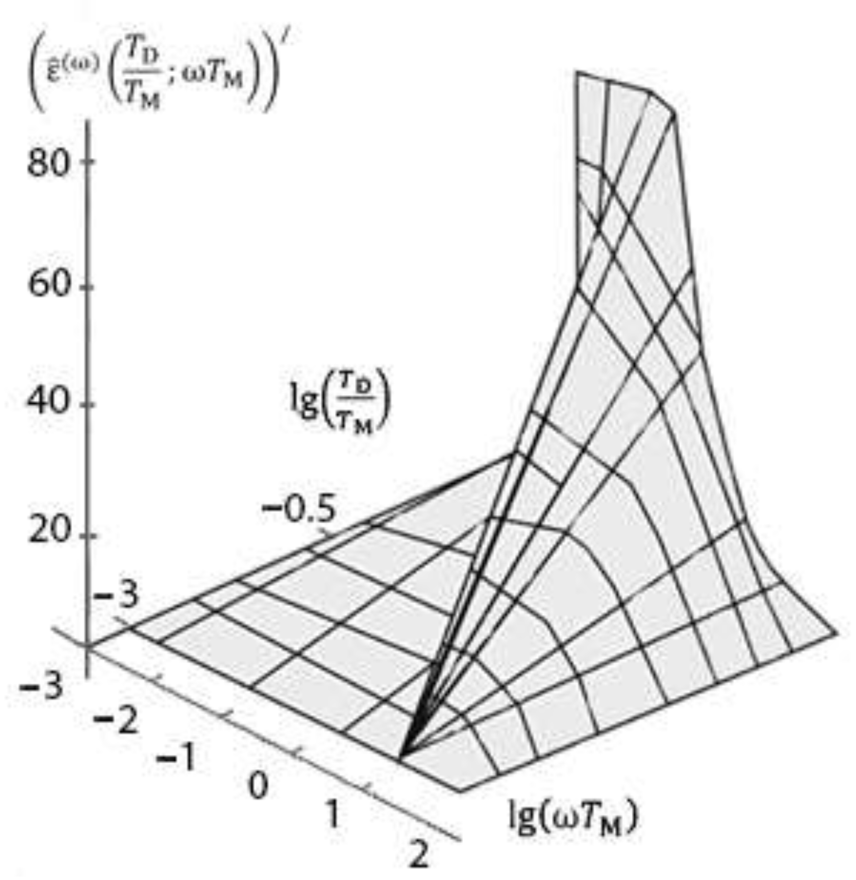
2.9. Complex Dielectric Permittivity
2.10 Quasi-Classical Dielectric Relaxation Functions
3. Results
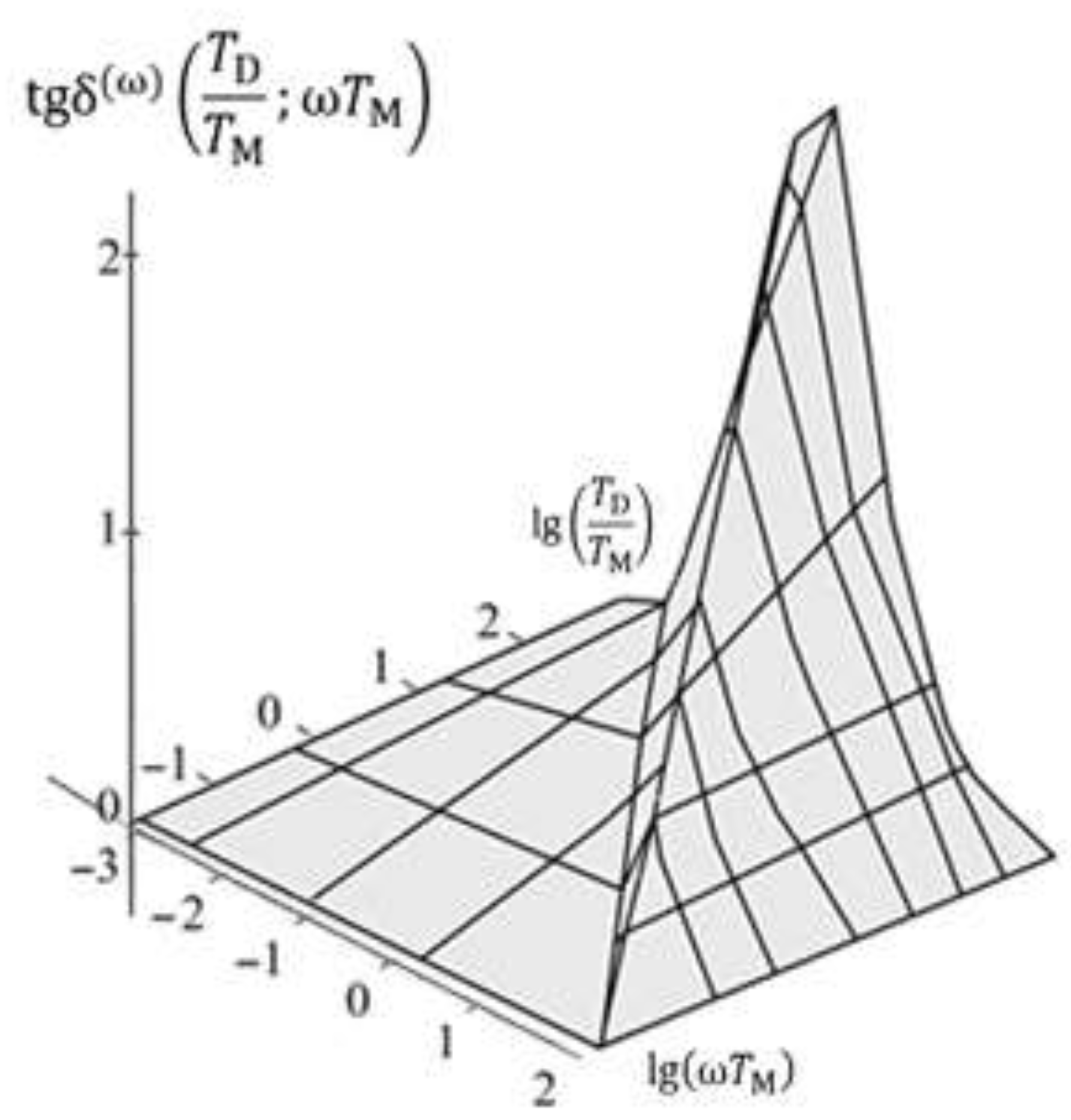
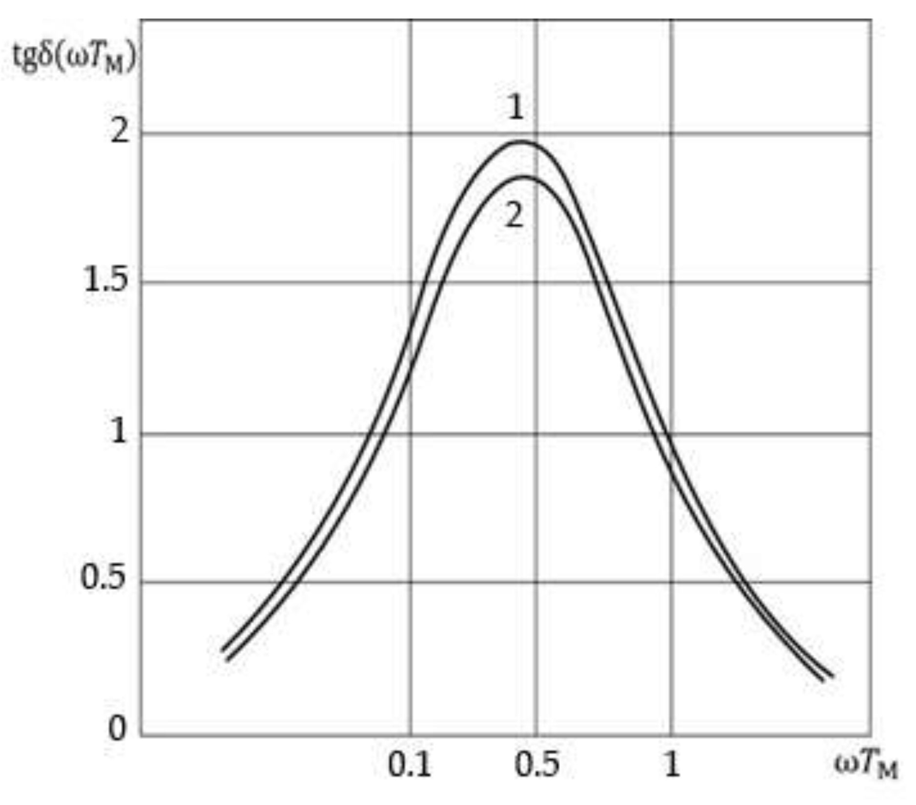
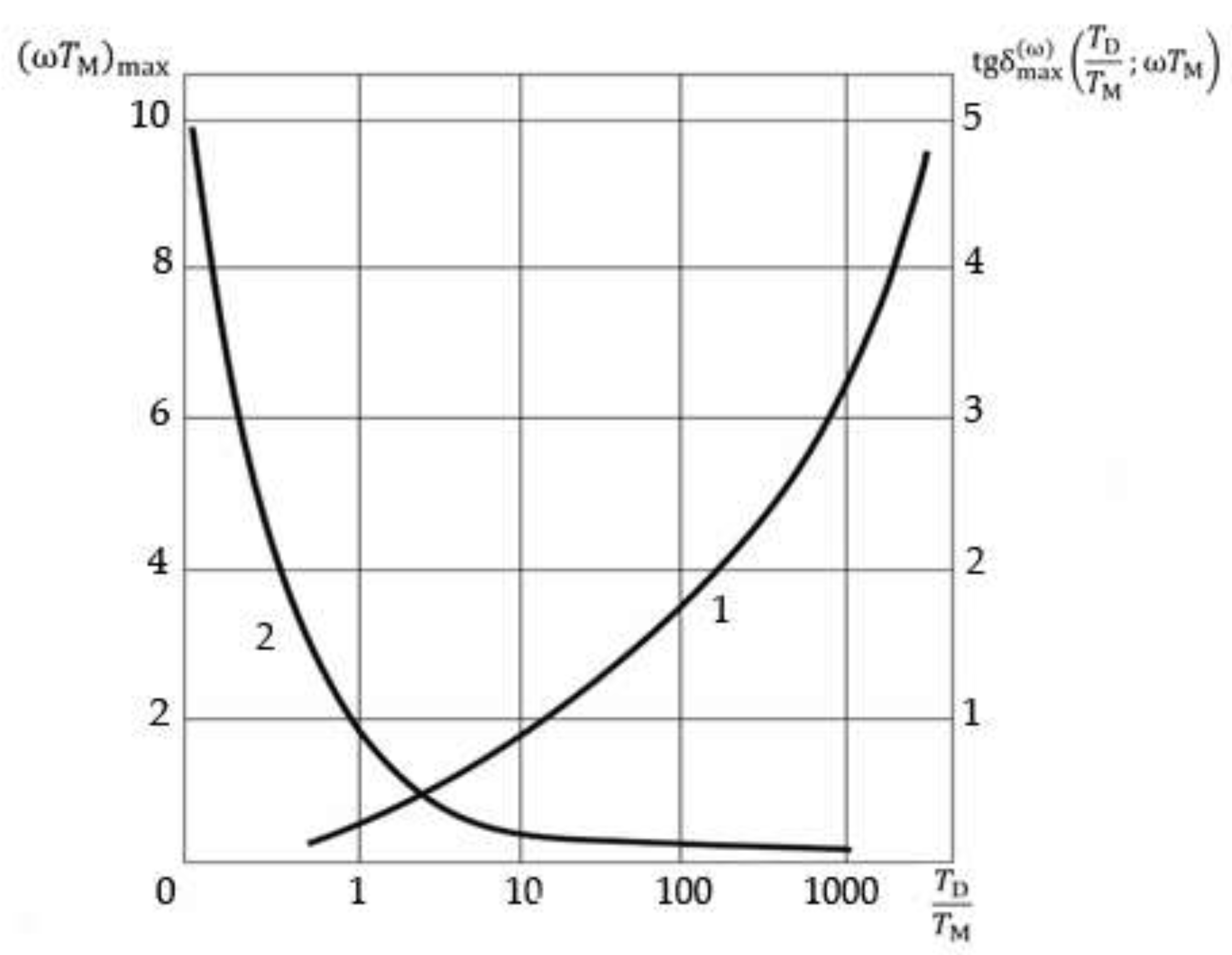
3.1. Dielectric Loss Tangent
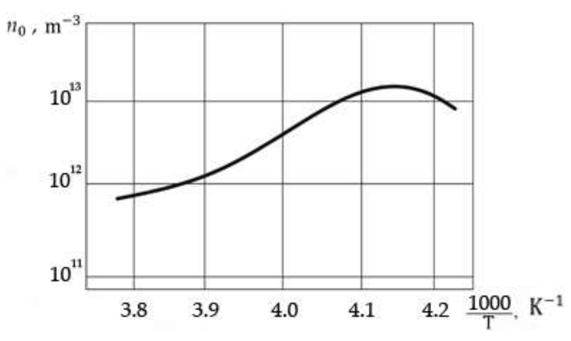
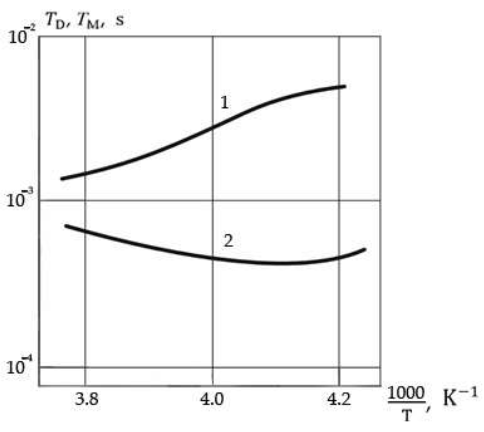
3.2. Comparative Analysis of Mechanisms of Maxwell and Diffusion Relaxation of Volumetric Charge

| Parameter name | Parameter values | ||||
| Temperature, Т, К | 234 | 238 | 245 | 255 | 264 |
| Relaxation time T |
2,64 | 2.34 | 2 | 1.72 | 1.69 |
| Low frequency Debye conductivity |
2 | 2.43 | 2.86 | 2.97 | 3.23 |
| Low frequency volumetric charge conductivity | 5 | 5.35 | 6.95 | 10 | 14.4 |
| Parameter name | Parameter values | ||||
| Temperature , T, K | 234 | 238 | 245 | 255 | 264 |
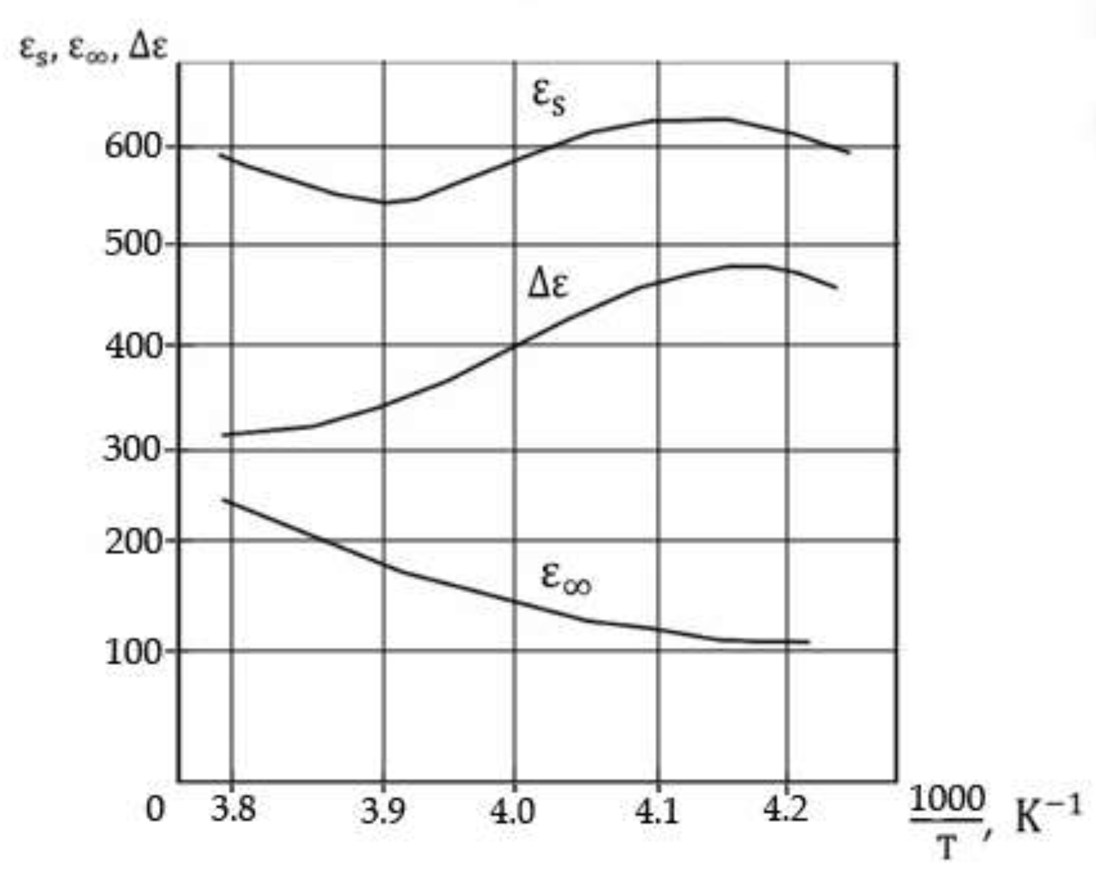
| Static dielectric constant см. фoрмул у (131) |
597 | 643 | 646 | 577 | 617 |
| High-frequency Debye conductivity | 149 | 141 | 157 | 194 | 275 |
| Dispersion depth |
448 | 502 | 489 | 383 | 342 |
| 4 | 4.56 | 4.11 | 2.97 | 2.24 | |
| Maxwell Relaxation Time, | 6.6 | 5.13 | 4.87 | 5.79 | 7.5 |
| 6.56 | 8.53 | 6.93 | 3.62 | 2.06 | |
| Diffusion relaxation time | 4.33 | 4.38 | 3.37 | 2.1 | 1.55 |
| Equilibrium concentration of mobile charge carriers, | 2.69 | 3.37 | 3.13 | 2.11 | 1.76 |
| Diffusion factor (the parameter is computed by (133)) |
9.5 | 9.4 | 12 | 19.5 | 26.5 |
| Mobility factor the parameter is computed by (134) |
4.64 | 4.5 | 5.7 | 8.78 | 11.5 |
4. Discussions
5. Conclusions
6. Patents
7. The Information About Previously Published Scientific Articles
Author Contributions
Funding
Institutional Review Board Statement
Informed Consent Statement
Data Availability Statement
Acknowledgments
Conflicts of Interest
Appendix A
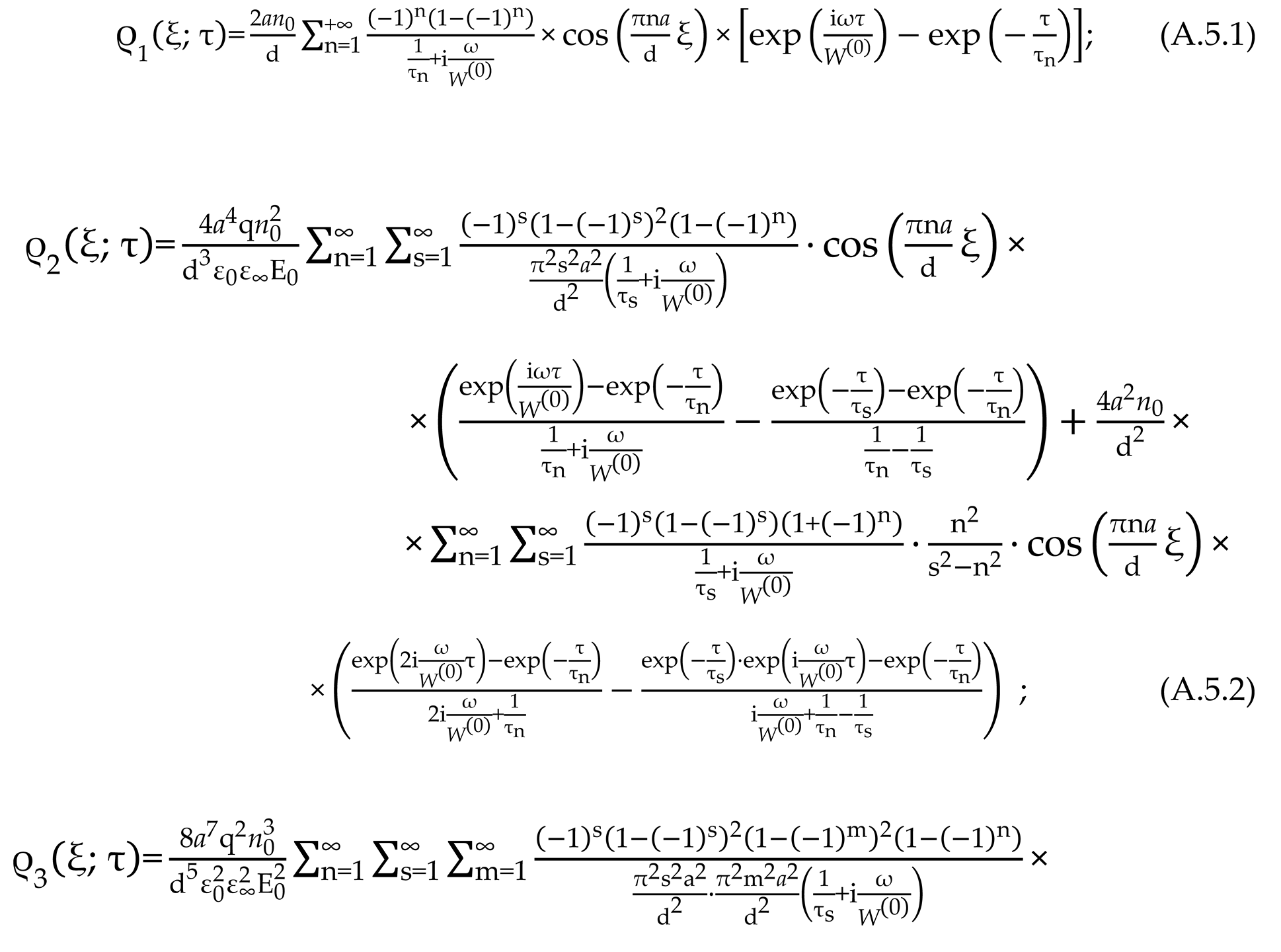
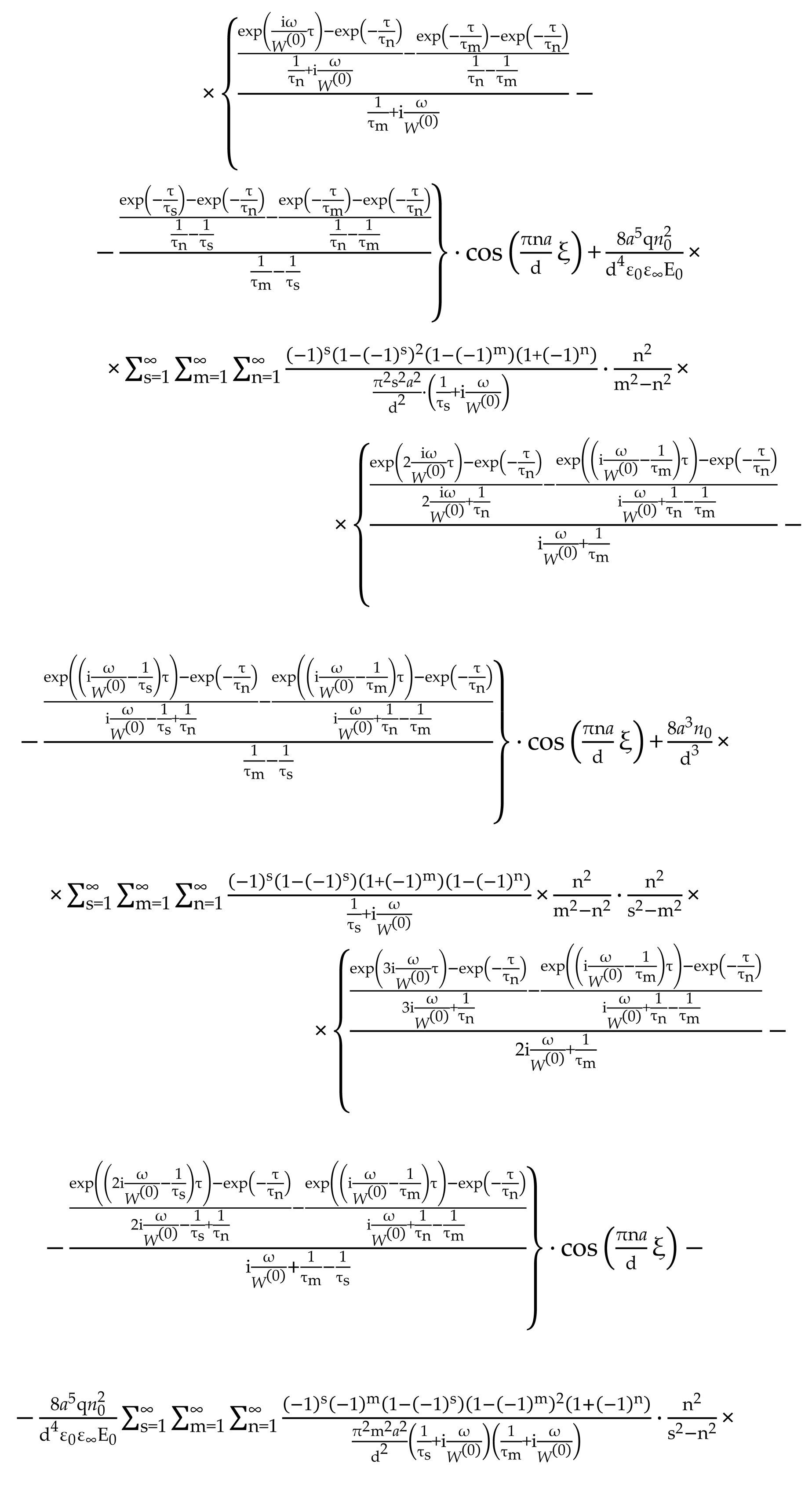
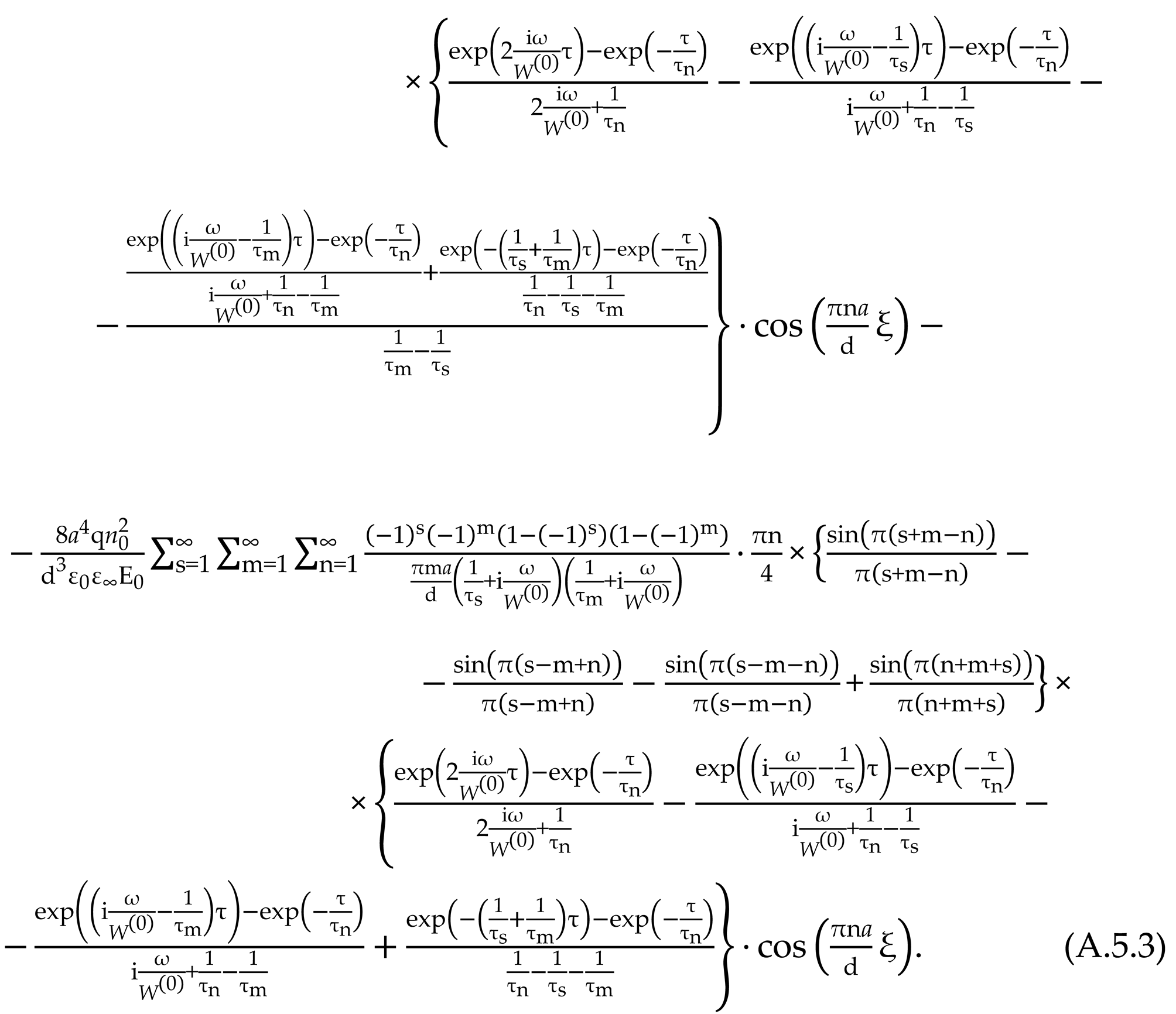
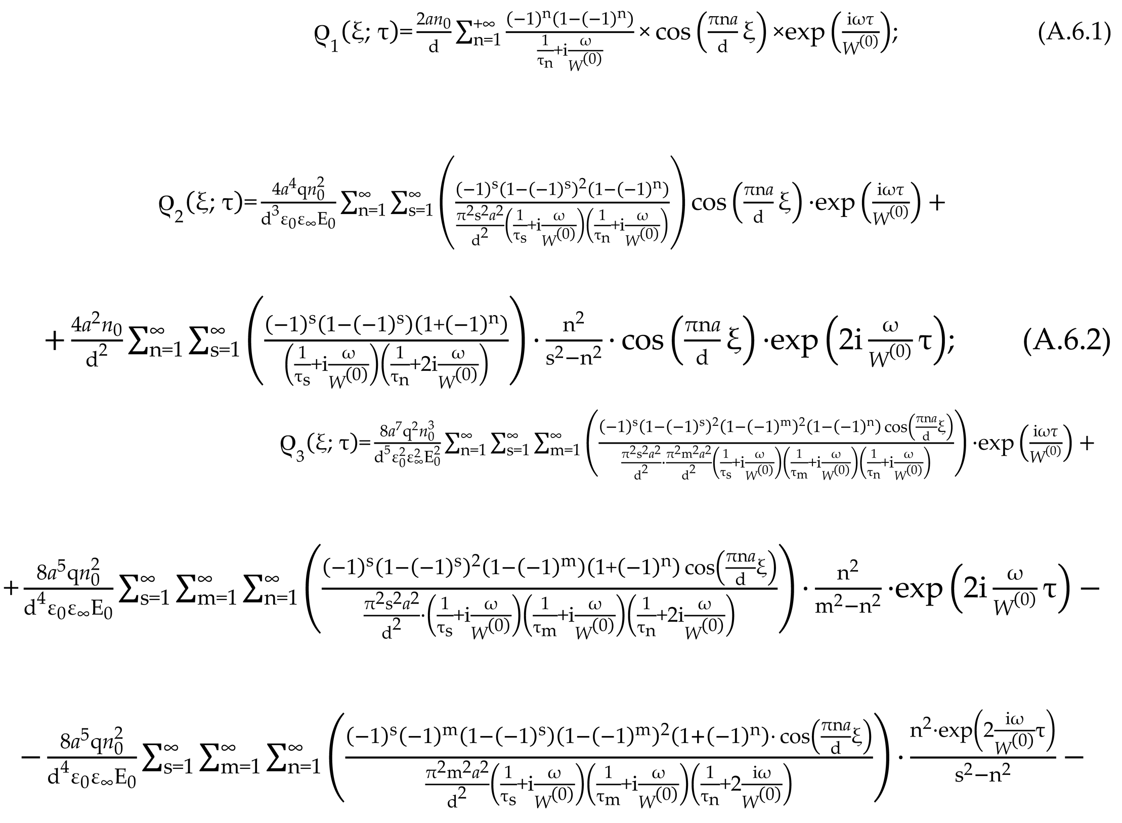
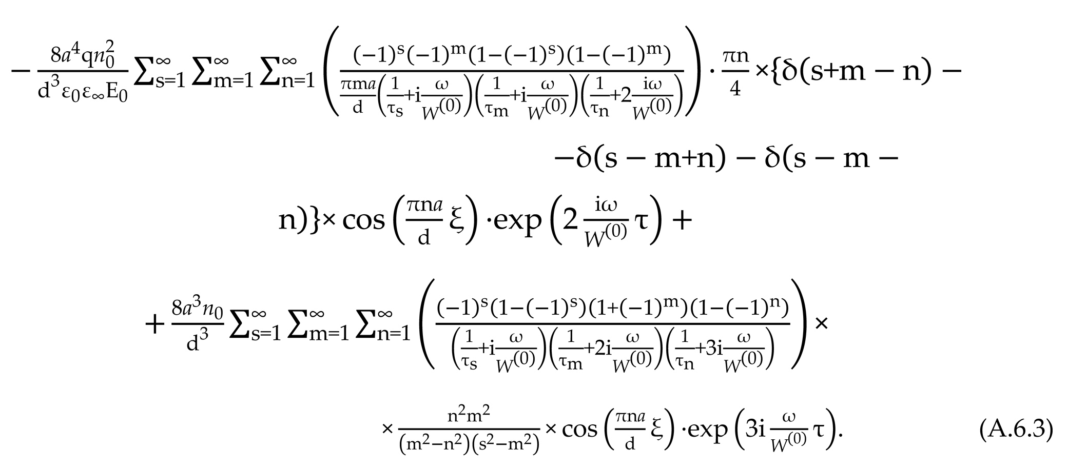
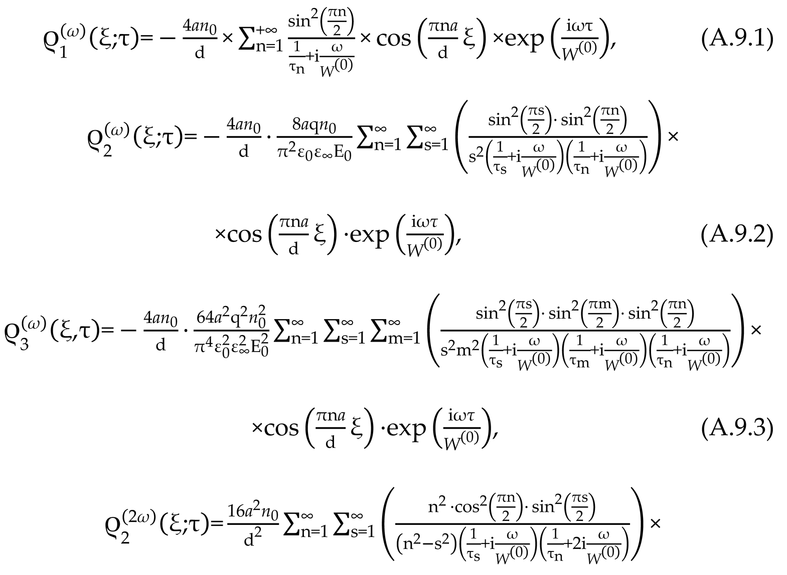
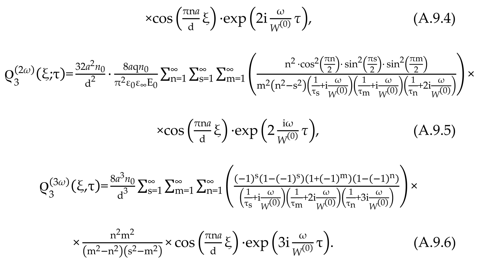
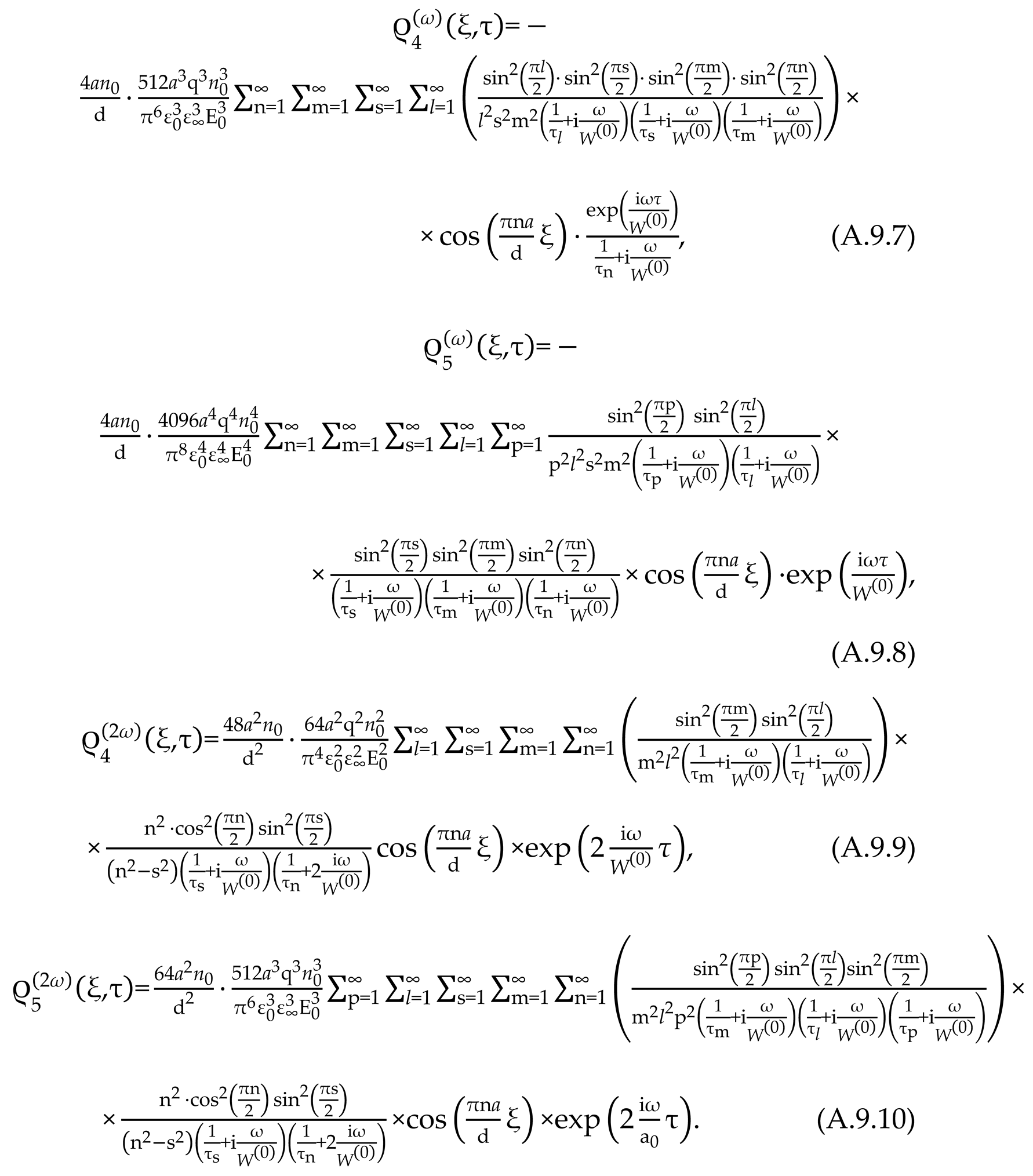
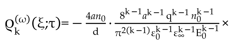
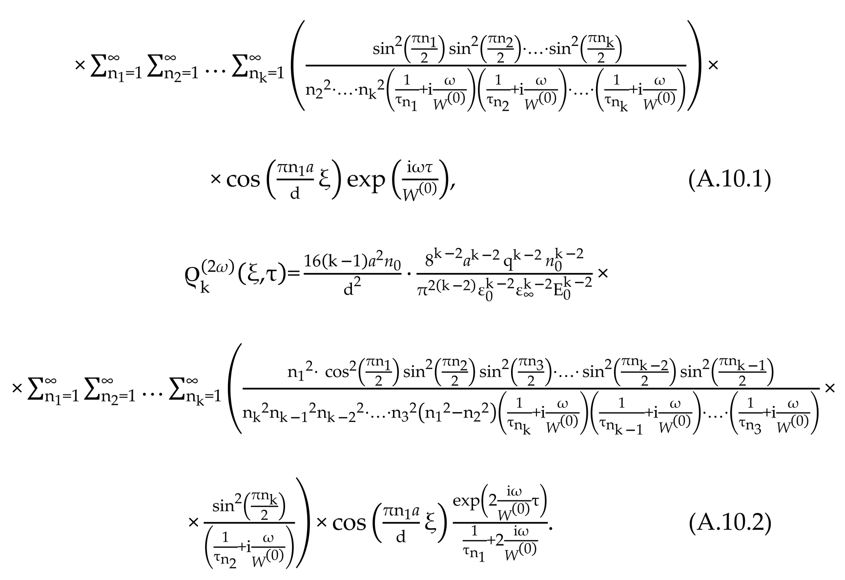
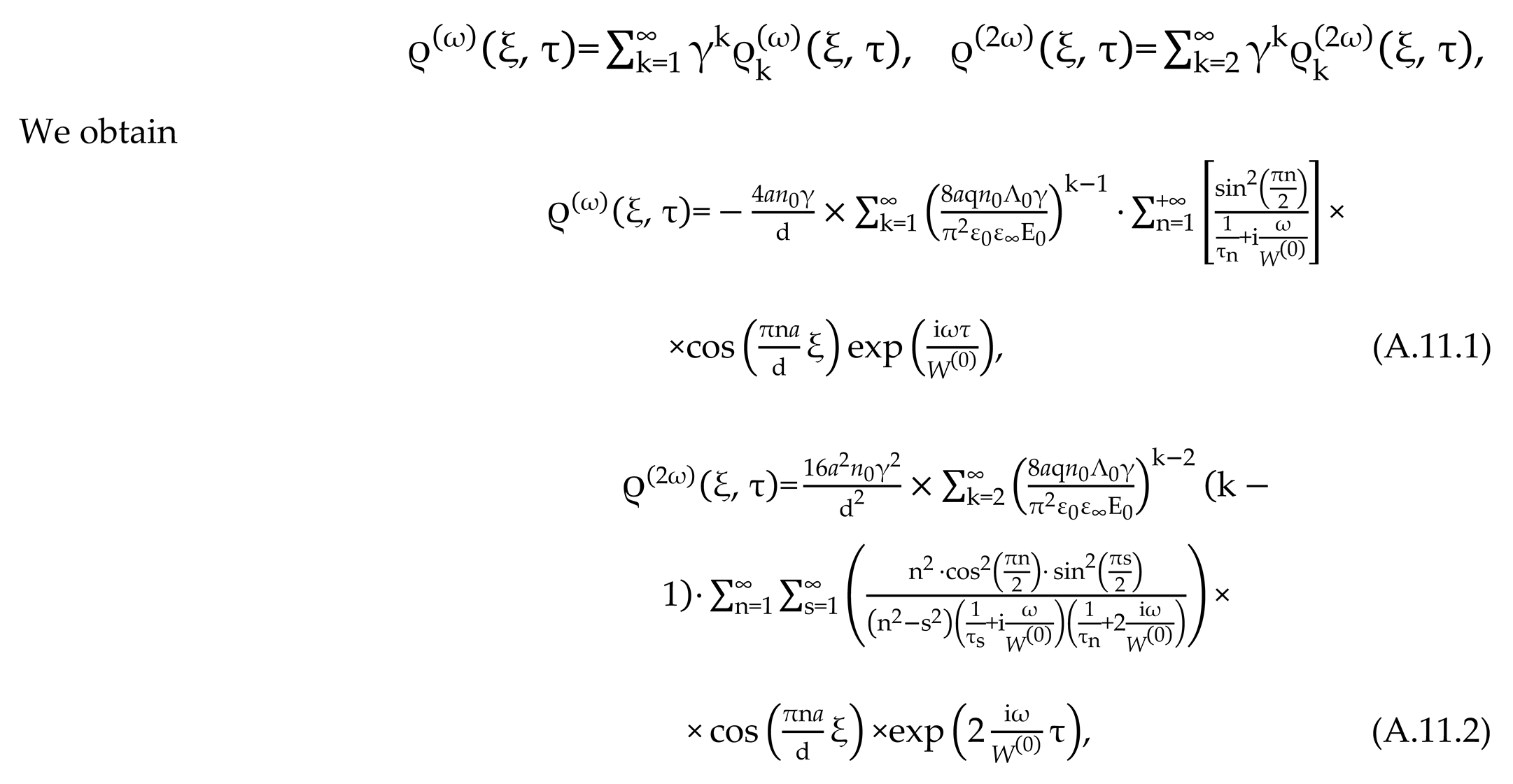 whence, we finally calculate the density of the volumetric charge in the function of the spatial variable and time in the infinite approximation of the perturbation theory , at the frequencies of the alternating electric field ,
 References
- Kalytka, V.A. Electrophysics of Proton Semiconductors and Dielectrics; Karaganda Technical University, KTU Publishing House: Karaganda, Kazahstan, 2021; Volume 133. [Google Scholar]
- Kalytka, V. , Bulatbayev, F., Neshina Y., Bilichenko, Y., Bilichenko, A., Bashirov, A., Sidorina, Y., Naboko, Y., Malikov, N., Senina, Y. Theoretical Studies of Nonlinear Relaxation Electrophysical Phenomena in Dielectrics with Ionic–Molecular Chemical Bonds in a Wide Range of Fields and Temperatures. Applied Sciences. Sect. Appl. Phys. 2022, 12, 35. [Google Scholar] [CrossRef]
- Kalytka, V. , Neshina, Y., Baimukhanov, Z., Mekhtiyev, A., Dunayev, P., Galtseva, O., Senina, Y. Influence of Quantum Effects on Dielectric Relaxation in Functional Electrical and Electric Energy Elements Based on Proton Semiconductors and Dielectrics. Applied Sciences. Sect. Appl. Phys. 2023. 13, 29. [CrossRef]
- Kalytka, V. , Mekhtiyev, A., Neshina, Y., Alkina, A. Aimagambetova, G.; Mukhambetov, R.; Bashirov, A. ; Afanasyev, D.; Bilichenko, A.; Zhumagulova, D. Physical and Mathematical Models of Quantum Dielectric Relaxation in Electrical and Optoelectric Elements Based on Hydrogen-Bonded Crystals. Crystals 2023, 13, 51. [Google Scholar] [CrossRef]
- Annenkov, Y.M.; Ivashutenko, A.S.; Vlasov, I.V.; Kabyshev, A.V. Electric properties of Coronado-Zirconium ceramics. Proc. Tomsk Polytech. Univ. 2005, 308, 35–38. [Google Scholar]
- Abrikosov, A.A. Resonance tunneling in high-temperature superconductors. UspekhiFiz. Nauk. 1998, 168, 683–695. [Google Scholar] [CrossRef]
- Panda, P.K. , Sahoo B. PZT to Lead Free Piezo Ceramics: A Review. Ferroelectrics. 2015, 474, 128–143. [Google Scholar] [CrossRef]
- Tonkonogov, M.P. Dielectric spectroscopy of hydrogen-bonded crystals, and proton relaxation. UspekhiFiz. Nauk. 1998, 41, 25–48. [Google Scholar] [CrossRef]
- Chang, L.; Esaki, L.; Tsu, R. Resonant tunneling in semiconductors double barrier. Appl. Phys. Lett. 1974, 24, 593–595. [Google Scholar] [CrossRef]
- Grodecka, A. , Machnikowski, P.Förstner, J. Phonon-assisted tunneling between singlet states in two-electron quantum dot molecules. Phys. Rev. B. 2008, 78, 085302. [Google Scholar] [CrossRef]
- Imry, Y. , Tinkham, M. Introduction to Mesoscopic Physics. Phys. Today. 1998, 51, 60–60. [Google Scholar] [CrossRef]
- Iogansen, L.V. On the possibility of resonant transfer of electrons in crystals through the barrier system. ZhETF. 1963, 45, 207–218. [Google Scholar]
- Iogansen, L. Thin-film electron interferometers. UspekhiFiz. Nauk. 1965, 86, 175–179. [Google Scholar] [CrossRef]
- Mattia, J.P. , McWhorter A.L., Aggarwal R.J., Rana F. Brown E.R.; Maki P. Comparison of a rate-equation model with experiment for the resonant tunneling diode in scattering-dominated regime. J. Appl. Phys. Lett. 1998, 84, 1140–1148. [Google Scholar]
- Pozdnyakov, A.A. , Sultanaev, R.M., Kiselev, V.I. Phenomenological theory of relaxation polarization of dielectrics. Russ. Phys. J. 1992, 35, 35–39. [Google Scholar] [CrossRef]
- Ktitorov, S.A. On the determination of the distribution function of relaxation times in terms of dielectric losses. Tech. Phys. Lett. 2003, 29, 22–74. [Google Scholar] [CrossRef]
- Marichev, V.A. Anomalous electrical conductivity of aqueous solutions in submicron cracks and gaps. J.Appl. Electrochem. 2005, 35, 17. [Google Scholar] [CrossRef]
- Pereira, L. , Mesquita, E., Alberto, N., Melo, J., Marques, C., Antunes, P., André, P.S., Varum, H. Fiber Bragg Grating Sensors for Reinforcing Bar Slippage Detection and Bond-Slip Gradient Characterization. Sensors. 2022, 22, 8866. [Google Scholar] [CrossRef]
- Wang, Y. , Yuan, H, Liu, X., Bai, Q.,Zhang, H., Gao, Y., Jin, B. A. Comprehensive Study of Optical Fiber Acoustic Sensing. IEEE Access 2019, 7, 85821–85837. [Google Scholar] [CrossRef]
- Udd, E. , W.B. The Emergence of Fiber Optic Sensor Technology. In Fiber Optic Sensors: An Introduction for Engineers and Scientists; Wiley: Hoboken, NJ, USA, 2011; pp. 1–8. [Google Scholar] [CrossRef]
- Mekhtiev, A.D. , Yurchenko, A.V., Ozhigin, S.G., Neshina, E.G., Al, A.D. Quasi-distributed fiber-optic monitoring system for overlying rock mass pressure on roofs of underground excavations. J. Min. Sci. 2021, 57, 354–360. [Google Scholar] [CrossRef]
- Wu, H. , Wan, Y., Tang, M., Chen, Y., Zhao, C., Liao, R., Chang, Y., Fu, S., Shum, P.P.;,Liu, D. Real-Time Denoising of Brillouin Optical Time Domain Analyzer with High Data Fidelity Using Convolutional Neural Networks. J. Light. Technol. 2019, 37, 2648–2653. [Google Scholar] [CrossRef]
- Madi, P.S. , Kalytka, V.A., Alkina, A.D., Nurmaganbetova, M.T. Development of a model fiber-optic sensor of the external action on the basis of diffraction gratings with variable parameters of the system. IOP Conf. Ser. J. Phys. 2019, 1327, 012036. [Google Scholar] [CrossRef]
- Neshina, Y. , Mekhtiyev, A., Alkina, A., Yugay, V., Kalytka V., Sarsikeyev, Y., Kirichenko L. Developing an Intelligent Fiber-Optic System for Monitoring Reinforced Concrete Foundation Structure Damage. Applied Sciences. Sect. Civil Engineering. 2023, 13, 23. [Google Scholar] [CrossRef]
- Neshina, Y. , Mekhtiyev, A., Kalytka, V., Kaliaskarov, N., Galtseva O., Kazambayev I. Fiber-Optic System for Monitoring Pit Collapse Prevention. Applied Sciences. Sect. Optics and Lasers. 2024, 14, 18. [Google Scholar] [CrossRef]
- D. Mekhtiyev, A. V. Yurchenko, V. A. Kalytka, Y. G. Neshina, A. D. Alkina, P. Sh. Madi. A Fiber-Optic Long-Base Deformometer for a System for Monitoring Rocks on the Sides of Quarries. Technical Physics Letters, 2022, 48, 30–32. [Google Scholar] [CrossRef]
- Belonenko, M.B. Characteristic features of nonlinear dynamics of a laser pulse in a photorefractive ferroelectric with hydrogen bonds. Quantum Electron. 1998, 28, 247–250. Available online: https://iopscience.iop.org/article/10.1070/QE1998v028n03ABEH001169. (accessed on 23 July 2023). [CrossRef]
- Volk, T. Ferroelectric phenomena in holographic properties of strontium-barium niobate crystals doped with rare-earth elements. Ferroelectrics. 1997, 203, 457–470. [Google Scholar] [CrossRef]
- Lebedev, N.G. , Litinsky, A.O. Model of an ion-embedded stoichiometric cluster for calculating the electronic structure of ionic crystals. Phys. Solid State. 1996, 38, 959–962. Available online: https://journals.ioffe.ru/articles/viewPDF/17380. (accessed on 23 July 2023).
- Abrahams, S.C. , Kurtz, S.K., Jamieson, P.B. Atomic displacement relationship to Curie temperature and spontaneous polarization in displacive ferroelectrics. Phys. Rev. 1968, 172, 551–553. [Google Scholar] [CrossRef]
- Kulagin, I.A. Components of the third-order nonlinear susceptibility tensors in KDP, DKDP and LiNbO3 nonlinear optical crystals. Quantum Electron. 2004, 34, 657. [Google Scholar] [CrossRef]
- V. S. Bystrov, E. V. Paramonova, X. Meng, H. Shen, J. Wang & V. M. Fridkin (2022) Polarization switching in nanoscale ferroelectric composites containing PVDF polymer film and graphene layers// Ferroelectrics, 2022, 590, 27-40. [CrossRef]
- Strukov, B.A. Levanyuk A.P. Ferroelectric Phenomena in Crystals. Physical Foundations; Springer: Berlin/Heidelberg. Germany, 1998; 308. [CrossRef]
- Fridkin, V.M. Critical size in ferroelectric nanostructures. Phys. Usp. 2006, 49, 193–202. [Google Scholar] [CrossRef]
- Levin, A.A. , Dolin S.P., Zaitsev A.R. Charge distribution, polarization and properties of ferroelectrics of type KDP. Chemical Physics 1996, 15. [Google Scholar]
- Movchikova, A. , Malyshkina, O.V., Pedko, B.B., Suchaneck, G.; Gerlach, G. Thermal wave study of piezoelectric coefficient distribution in PMN-PT single crystals. Adv. Appl. Ceram. 2010, 109, 131–134. [Google Scholar] [CrossRef]
- Mukhortov, V.M. , Golovko, Y.I., Mamatov, A.A., Zhigalina, O.M., Kuskova, A.N., Chuvilin, A.L. Influence of Internal Deformation Fields on the Controllability of Nanosized Ferroelectric Films in a Planar Capacitor. Tech. Phys. Lett. 2010, 80, 77–82. [Google Scholar]
- Movchikova, A.A.; Malyshkina, O.V.; Pedko, B.B.; Lisitsin, V.S.; Burtsev, A.V. Influence of thermocycling on the polarization distribution of doped SBN crystals. Ferroelectrics. 2010, 399, 14–19. [Google Scholar] [CrossRef]
- Efremova, P.V.; Ped’ko, B.B.; Kuznecova, Y.V. Structural examination of lithium niobate ferroelectric crystals by combining scanning electron microscopy and atomic force microscopy. Tech. Phys. Lett. 2016, 61, 313–315. [Google Scholar] [CrossRef]
- Yaroslavtsev, A.B. Ion Diffusion Throw Interface in Heterogeneous Solid Systems with the Modified Surface. Defect Diffus. Forum. 2003, 216, 133–140. [Google Scholar] [CrossRef]
- Dadayan, A.K.; Borisov, Y.A.; Yu. A.; Zolotarev; Bocharov, E.V.; Nagaev, I.Y.; Myasoedov, N.F. Solid-State Catalytic Hydrogen/Deuterium Exchange in Mexidol Russ. J. Phys. Chem. 2021, 95, 273–278. [Google Scholar] [CrossRef]
- Yaroslavtsev, A.B. Perfluorinated ion-exchange membranes. Polym. Sci. Ser. A. 2013, 55, 674–698. [Google Scholar] [CrossRef]
- Prokopova, L.; Novotny, J.; Micka, Z.; Malina, V. Growth of TriglycineSulphate Single Crystal Doped by Cobalt (II) Phosphate. Cryst. Res. Technol. 2001, 36, 1189–1195. [Google Scholar] [CrossRef]
- Ragahvan, C.M.; Sankar, R.; Mohankumar, R.; Jayavel, R. Effect of Amino Acid Doping on The Growth and Ferroelectric Properties of TriglycineSulphate Single Crystals. Mater. Res. Bull. 2008, 43, 305–311. [Google Scholar] [CrossRef]
- Sun, X.; Wang, M.; Pan, Q.W.; Shiw; Fang, C. S. Study on the Growth and Properties of Guanidine Doped Triglycine Sulfate Crystal. Cryst. Res. Technol. 1999, 34, 1251–1254. [Google Scholar] [CrossRef]
- Yaroslavtsev, A.B. Solid electrolytes: Main prospects of research and development. Russ. Chem. Rev. 2016, 85, 1255–1276. [Google Scholar] [CrossRef]
- Yaroslavtsev, A.B. Proton conductivity of inorganic hydrates. Russ. Chem. Rev. 1994, 63, 429–435. [Google Scholar] [CrossRef]
- Gaffar, M.A.; Al-Fadl, A.A. Effect of Doping and Irradiation on Optical Parameters of TriglycineSulphate Single Crystals. Cryst. Res. Technol. 1999, 34, 915–923. [Google Scholar] [CrossRef]
- Farhana, K.; Jiban, P. Structural and Optical Properties of Triglycine Sulfate Single Crystals Doped with Potassium Bromide. J. Cryst. Process Technol. 2011, 1, 26–31, https://www.scirp.org/html/3-1010007_6553.htm. [Google Scholar] [CrossRef]
- Strukov, B.A.; Yakushkin, E.D. Local sound velocity and growth defects in triglycinesulfate crystals. Phys. Solid State 1978, 20, 1551–1553. [Google Scholar]
- Shut, V.N.; Kashevich, I.F.; Syrtsov, S.R. Ferroelectric Properties of Triglycine Sulfate Crystals with a Non-uniformdistribution of Chromium Impurities. Phys. Solid State 2008, 50, 118–121. [Google Scholar] [CrossRef]
- Genbo, S.; Youping, H.; Hongshi, Y.; Zikong, S.; Qingin, E. A New Pyroelectric Crystal Lysine-Doped TGS (LLTGS). J. Cryst. Growth. 2000, 209, 220–222. [Google Scholar] [CrossRef]
- Aravazhi, S.; Jayavel, R.; Subramanian, C. Growth and Characterization of H-Benzophenone and Urea Doped TriglycineSulphate Crystals. Ferroelectrics. 1997, 200, 279–286. [Google Scholar] [CrossRef]
- M. B. Okatan, J.V. Mantese, S.P. Alpay.Effect of space charge on the polarization hysteresis characteristics of monolithic and compositionally graded ferroelectrics. Acta Materialia. 2010, 58, 39–48. [Google Scholar]
- Prasolov, B.N.; Safonova, I.A. Influence of the rate and direction of passage of a second-order phase transition on dielectric losses in TGS-crystals. Proceedings of the Academy of Sciences of the USSR. Series "Physics". 1993, 57, 47–49. [Google Scholar]
- RogazinskayaO. V.;MilovidovaS.D.;SidorkinA.S.;ChernyshevV.V.;BabichevaN.G. Properties of nanoporous alumina with inclusions of triglycine sulfate and rochellesalt. Physics of the Solid State. 2009, 51, 1430. [Google Scholar]
- TryukhanT. A.; Stukova E.V.;Baryshnikov S.V. Dielectric properties triglitsinsulfat in porous matrices. Academic Journal “Izvestia of Samara Scientific Center of the Russian Academy of Sciences”, Series: Physics and Electronics. 2010, 12, 4. [Google Scholar]
- Stankowska, J.; Czosnowska, E. Effect of grown conditions on the domain structure of triglycine sulphate crystals. ActaPhys.Polon. 1975, 43, 641–644. [Google Scholar]
- Park, J.H.; Kim, H.Y.; Seok, K.H.; Kiaee, Z.; Lee, S.K.; Joo, S.K. Multibit ferroelectric field-effect transistor with epitaxial-like Pb(Zr, Ti)O3. J. Appl. Phys. 2016, 119, 124108. [Google Scholar] [CrossRef]
- Park, J.H.; Joo, S.K. A Novel Metal-Ferroelectric-Insulator-Silicon FET With Selectively Nucleated Lateral Crystallized Pb (Zr,Ti)O3 and ZrTiO4 Buffer for Long Retention and Good Fatigue. IEEE Electron.DeviceLett. 2015, 36, 1033–1036. [Google Scholar] [CrossRef]
- Hu, J.M.; Chen, L.Q.; Nan, C.W. Multiferroichetero structures integrating ferroelectric and magnetic materials. Adv. Mater. 2016, 28, 15–39. [Google Scholar] [CrossRef]
- Magdău, I.B.; Liu, X.-H.; Kuroda, M.A.; Shaw, T.M.; Crain, J.; Solomon, P.M.; Newns, D.M.; Martyna, G.J. The piezoelectronic stress transduction switch for very large-scale integration, low voltage sensor computation, and radio frequency applications. Appl. Phys. Lett. 2015, 107, 073505. [Google Scholar] [CrossRef]
- Kayumov, D. , Bulatbaev F., Kayumova I., Breido J., Bulatbayeva Y.AN ENGINEERING APPROACH FOR THE QUALITATIVE ASSESSMENT OF THE LUMINOUS FLUX OF LED LAMPS. International Journal of Energy for a Clean Environment. 2023, 24, 31–43. [Google Scholar] [CrossRef]
- Mekhtiyev, A.D. , Bulatbayev F.N., Taranov A.V., Bashirov A.V, Neshina Y.G., Alkina A.D. Use of reinforcing elements to improve fatigue strength of steel structures of mine hoisting machines (MHM). Metalurgija. 2020, 59, 121–124. [Google Scholar]
- Yurchenko, A.V. , Mekhtiyev, A.D., Bulatbaev, F.N., Alkina, A.D., Sh Madi, P. Investigation of additional losses in optical fibers under mechanical action. IOP Conference Series: Materials Science and Engineering 2019, 516, 012004. [Google Scholar] [CrossRef]
- Skinner S., J. Recent advances in Perovskite-type materials for solid oxide fuel cell cathodes. International Journal Of Inorganic Materials. 2001, 3, 113–121. [Google Scholar] [CrossRef]
- Kalytka, V.А.; Korovkin, М.V. Quantum Effects at a Proton Relaxation at Low Temperatures. Russian Phys. J. 2016, 59, 994–1001. [Google Scholar] [CrossRef]
- Kalytka, V.A.; Korovkin, M.V. Dispersion Relations for Proton Relaxation in Solid Dielectrics. Russian Phys. J. 2017, 59, 2151–2161. [Google Scholar] [CrossRef]
- Kalytka,V. A.; Mekhtiev,A.D.; Bashirov,A.; Yurchenko,A.V.; Al’Kina,A.D. Nonlinear Electrophysical Phenomena in Ionic Dielectrics with a Complicated Crystal Structure. Russian Phys. J. 2020, 63, 282–289. [Google Scholar] [CrossRef]
- Annenkov, Y.M.; Kalytka, V.; Korovkin, M.V. Quantum Effects Under Migratory Polarization in Nanometer Layers of Proton Semiconductors and Dielectrics at Ultralow Temperatures. Russian Phys. J. 2015, 58, 35–41. [Google Scholar] [CrossRef]
- Kalytka, V.A.; Korovkin, M.V.; Mekhtiyev, A.D.; Yurchenko, A.V. Nonlinear Polarization Effects in Dielectrics with Hydrogen Bonds. Russ. Phys. J. 2018, 61, 757–769. [Google Scholar] [CrossRef]
- Kalytka, V.A. The mathematical description of the nonlinear relaxation of polarization in dielectrics with hydrogen bonds. Bull. Samara University. Nat. Sci. Ser. 2017, 23, 71–83. [Google Scholar] [CrossRef]
- Kalytka, V.A. Nonlinear kinetic phenomena under polarization in solid dielectrics. Bull. Mosc. Reg. State Univ. Ser. Phys. Math. 2018, 2, 61–75. [Google Scholar] [CrossRef]
- Kalytka, V.A.; Bashirov, A.V.; Tatkeyeva, G.G.; Sidorina, Y.A.; Ospanov, B.S.; Ten, T.L. The impact of the nonlinear effects on thermally stimulated depolarization currents in ion dielectrics. Period. Eng. Nat. Sci. 2021, 9, 195–217. [Google Scholar] [CrossRef]
- Kalytka, V.A. Investigating the scheme of numerical calculation the parameters of non-linear electrophysical processes by minimizing comparison function method. Space Time Fundam. Interact. 2018, 3, 68–77. Available online: https://stfi.ru/ru/issues/2018/03/STFI_2018_03_Kalytka.html (accessed on 23 July 2023). [CrossRef]
- Kalytka, V.A.; Korovkin, M.V.; Madi, P.S.; Kalacheva, S.A.; Sidorina, Y.A. Universal installation for studying structural defects in electrical and optical fiber materials. IOP Conf. Ser. J. Phys. 2020, 1499, 012046. [Google Scholar] [CrossRef]
- Kalytka, V.; Korovkin, M.V.; Madi, P. S. , Magauin, B.K.; Kalinin, A.V.;Sidorina, Y.A. Quantum-mechanical model of thermally stimulated depolarization in layered dielectrics at low temperatures. IOP Conf. Ser. J. Phys. 2021, 1843, 012011. [Google Scholar] [CrossRef]
- Valeriy Kalytka, Mikhail Korovkin, Galina Tatkeyeva, Aleksandr Bashirov, Yekaterina Bilichenko, Yelena Sidorina, Yelena Senina, Bektas Ospanov, Dana Brazhanova, Galym Baidyussenov, Nursultan Seitzhapparov. QUANTUM KINETIC PHENOMENA IN PROTON SEMICONDUCTORS AND DIELECTRICS // The 3rd International Conference on "FUNCTIONAL MATERIALS AND CHEMICAL ENGINEERING, City Seasons Suites, Dubai, UAE, November 09-10, 2022, pp. 95-97.
- Ronald, E. Cohen. Surface effects in ferroelectrics: Periodic slab computations for BaTiO3. Ferroelectrics 1997, 194, 323–342. [Google Scholar] [CrossRef]
- Taibarei Nikolai, O. , Kytin Vladimir G., Konstantinova Elizaveta A., Kulbachinskii Vladimir A., Shalygina Olga A., Pavlikov Alexander V., Savilov Serguei V., Tafeenko Viktor A., Mukhanov Vladimir A., Solozhenko Vladimir L., Baranov Andrei N. Doping Nature of Group V Elements in ZnO Single Crystals Grown from Melts at High Pressure. Crystal Growth and Design 2022, 22, 2452–2461. [Google Scholar] [CrossRef]
- Ezhilvalavan, S. , Tseng T.-Y. Progress in the developments of (Ba,Sr)TiO3 (BST) thin films for Gigabitera DRAMs. Materials Chemistry and Physics 2000, 65, 227–248. [Google Scholar] [CrossRef]
- Huber, S.P. , Zoupanos, S., Uhrin, M. et al. AiiDA 1.0, a scalable computational infrastructure for automated reproducible workflows and data provenance. Science Data 2020, 7, 300. Available online: https://www.nature.com/articles/s41597-020-00638-4.pdf. [CrossRef]
- Boris, A. Strukov, Arkadi P. Levanyuk. Ferroelectric Phenomena in Crystals. Physical Foundations.2 Publisher: Springer Berlin, Heidelberg. 1998. 308. [CrossRef]
- Сhang, J.B.; Miyazoe, H.; Copel, M.; Solomon, P.M.; Liu, X.-H.; Shaw, T.M.; Schrott, A.G.; Gignac, L.M.; Martyna, G.J.; Newns, D.M. First realization of the piezo-electronic stress-based transduction device. Nanotechnology. 2015, 26, 375201. [Google Scholar] [CrossRef]
- Newns, D.; Elmegreen, B.; Liu, X.H.; Martyna, G.J. A low-voltage high-speed electronic switch based on piezoelectric transduction. J. Appl. Phys. 2012, 111, 084509. [Google Scholar] [CrossRef]
- Newns, D.M.; Elmegreen, B.G.; Liu, X.H.; Martyna, G.J. High response piezoelectric and piezoresistive materials for fast, low voltage switching: Simulation and theory of transduction physics at the nanometer-scale. Adv. Mater. 2012, 24, 3672–3677. [Google Scholar] [CrossRef]
- Newns, D.M.; Elmegreen, B.G.; Liu, X.H.; Martyna, G.J. The piezoelectronic transistor: A nanoactuator-based post-CMOS digital switch with high speed and low power. MRS Bull. 2012, 37, 1071–1076. [Google Scholar] [CrossRef]
- Doh, Y.J.; Yi, G.C. Nonvolatile memory devices based on few-layer graphene films. Nanotechnology. 2010, 21, 105204. [CrossRef] [PubMed]
- Xie, L.; Chen, X.; Dong, Z.; Yu, Q.; Zhao, X.; Yuan, G.; Zeng, Z.; Wang, Y.; Zhang, K. Nonvolatile Photoelectric Memory Induced by Interfacial Charge at a Ferroelectric PZT-Gated Black Phosphorus Transistor. Adv. Electron.Mater. 2019, 5, 1900458. [Google Scholar] [CrossRef]
- Shen, P.C.; Lin, C.; Wang, H.; Teo, K.H.; Kong, J. Ferroelectric memory field-effect transistors using CVD monolayer MoS2 as resistive switching channel. Appl. Phys. Lett. 2020, 116, 033501. [Google Scholar] [CrossRef]
- McGuire, F.A.; Lin, Y.C.; Price, K.; Rayner, G.B.; Khandelwal, S.; Salahuddin, S.; Franklin, A.D. Sustained sub-60 mV/decade switching via the negative capacitance effect in MoS2 transistors. Nano Lett. 2017, 17, 4801–4806. [Google Scholar] [CrossRef]
- Alam, M.A.; Si, M.; Ye, P.D. A critical review of recent progress on negative capacitance field-effect transistors. Appl. Phys. Lett. 2019, 114, 090401. [Google Scholar] [CrossRef]
- Stadler, H.L. Ferroelectric switching time of BaTiO3 crystals at high voltages. J. App. Phys. 1958, 29, 1485–1487. [Google Scholar] [CrossRef]
- Scott, J.F.; McMillan, L.D.; Araujo, C.A. Switching kinetics of lead zirconatetitanate sub-micron thin-film memories. Ferroelectrics. 1989, 93, 31–36. [Google Scholar] [CrossRef]
- Li, J.; Nagaraj, B.; Liang, H.; Cao, W.; Lee, C.H.; Ramesh, R. Ultrafast polarization switching in thin-film f1erroelectrics. Appl. Phys.Lett. 2004, 84, 1174–1176. [Google Scholar] [CrossRef]
- Ishii, H.; Nakajima, T.; Takahashi, Y.; Furukawa, T. Ultrafast polarization switching in ferroelectric polymer thin films at extremely high electric fields. Appl. Phys. Express. 2011, 4, 031501. [Google Scholar] [CrossRef]
- Mulaosmanovic, H.; Ocker, J.; Muller, S.; Schroeder, U.; Muller, J.; Polakowski, P.; Slesazeck, S. Switching kinetics in nanoscale hafnium oxide based ferroelectric field-effect transistors. ACS Appl. Mater. Interfaces. 2017, 9, 3792–3798. [Google Scholar] [CrossRef] [PubMed]
- Liu, Z.Q.; Liu, J.H.; Biegalski, M.D.; Hu, J.M.; Shang, S.L.; Ji, Y.; Wang, J.M.; Hsu, S.L.; Wong, A.T.; Cordill, M.J.; et al. Electrically reversible cracks in an intermetallic film controlled by an electric field. Nat. Commun. 2018, 9, 41. [Google Scholar] [CrossRef] [PubMed]
- Oh, S.; Hwang, H.; Yoo, I.K. Ferroelectric materials for neuromorphic computing. APL Mater. 2019, 7, 091109. [Google Scholar] [CrossRef]
- Ishibashi, Y.; Takagi, Y. Note on ferroelectric domain switching. J. Phys. Soc. Jpn. 1971, 31, 506–510. [Google Scholar] [CrossRef]
- Ishiwara, H. Proposal of adaptive-learning neuron circuits with ferroelectric analog-memory weights. Jpn. J. Appl. Phys. 1993, 32, 442–446. [Google Scholar] [CrossRef]
- Jerry, M.; Dutta, S.; Kazemi, A.; Ni, K.; Zhang, J.; Chen, P.Y.; Datta, S. A ferroelectric field effect transistor based synaptic weight cell. J. Phys. D: Appl. Phys. 2018, 51, 434001. [Google Scholar] [CrossRef]
- Seo, M.; Kang, M.H.; Jeon, S.B.; Bae, H.; Hur, J.; Jang, B.C.; Hwang, K.M. First demonstration of a logic-process compatible junctionless ferroelectric FinFET synapse for neuromorphic applications. IEEE Electr. Device Lett. 2018, 39, 1445–1448. [Google Scholar] [CrossRef]
- Kim, M.K.; Lee, J.S. Ferroelectric analog synaptic transistors. Nano Lett. 2019, 19, 2044–2050. [Google Scholar] [CrossRef]
- Boyn, S.; Grollier, J.; Lecerf, G.; Xu, B.; Locatelli, N.; Fusil, S.; Girod, S.; Carretero, C.; Garcia, K.; Xavier, S.; et al. Learning through ferroelectric domain dynamics in solid-state synapses. Nat. Commun. 2017, 8, 1–7. [Google Scholar] [CrossRef]
- Park, M.H.; Lee, Y.H.; Kim, H.J.; Kim, Y.J.; Moon, T.; Kim, K.D.; Müller, J.; Kerch, A.; Schroeder, U.; Mikolajick, T.; et al. Ferroelectricity and Antiferroelectricity of Doped Thin HfO2-Based Films. Adv. Mater. 2015, 27, 1811–1831. [Google Scholar] [CrossRef]
- Müller, J.; Böscke, T.S.; Bräuhaus, D.; Schröder, U.; Böttger, U.; Sundqvist, J.; Kücher, P.; Mikolajick, T.; Frey, L. Ferroelectric Zr0.5Hf0.5O2 thin films for nonvolatile memory applications. Appl. Phys. Lett. 2011, 99, 112901. [Google Scholar] [CrossRef]
- Lee, S.-S.; Noh, K.-H.; Kang, H.-B.; Hong, S.-K.; Yeom, S.-J.; Park, Y.-J. Characterization of Hynix 16M FERAM adopted novel sensing scheme. Integr. Ferroelectrics 2003, 53, 343–351. [Google Scholar] [CrossRef]
- Malyshkina, O.V.; Movchikova, A.A.; Pedko, B.B.; Boitsova, K.N.; Kiselev, D.A.; Kholkin, A.L. Influence of Eu and Rh impurities on distribution of polarization of strontium-barium niobate crystals. Ferroelectrics. 2008, 373, 114–120. [Google Scholar] [CrossRef]
- Kapphan, S.; Pankrath, R.; Kislova, I.; Pedko, B.; Trepakov, V.; Savinov, M. Variation of doping-dependent properties in photorefractive SrxBa(1-x)Nb2O6:Ce,Cr,Ce+Cr. Radiat. Eff. Defects Solids. 2002, 157, 1033–1037. [Google Scholar] [CrossRef]
- Arimoto, Y.; Ishiwara, H. Current status of ferroelectric random-access memory. MRS Bull. 2004, 29, 823–828. [Google Scholar] [CrossRef]
- Moise, T.S.; Summerfelt, S.R.; McAdams, H.; Aggarwal, S.; Udayakumar, K.R.; Celii, F.G.; Martin, J.S. ;XingG.; Hall, L.; Taylor, K.J.; Hurd, T.; et al. Demonstration of a 4 Mb, high density ferroelectric memory embedded within a 130 nm, 5 LM Cu/FSG logic process. In Proceedings of the International Electron Devices Meeting (IEDM'02), San Francisco, CA, USA, 8–11 December 2002, 535–538. [CrossRef]
- Rodriguez, J.A.; Remack, K.; Boku, K.; Udayakumar, K.R.; Aggarwal, S.; Summerfelt, S.R.; Celii, F.G.; Martin, S.; Hall, L.; Taylor, K.; et al. Reliability properties of low voltage ferroelectric capacitors and memory arrays. IEEE Trans. Device Mater. Reliab. 2004, 4, 436–449. [Google Scholar] [CrossRef]
- Kim, K.; Lee, S. Integration of lead zirconium titanate thin films for high density ferroelectric random access memory. J. Appl. Phys. 2006, 100, 051604. [Google Scholar] [CrossRef]
- Park, Y.; Lee, J.H.; Koo, J.M.; Kim, S.P.; Shin, S.; Cho Ch., R.; Lee, J.K. Preparation of Pb(ZrxTi1-x)O3 films on trench structure for high-density ferroelectric random access memory. Integral Ferroelectr. 2004, 66, 85–95. [Google Scholar] [CrossRef]
- Shin, S.; Han, H.; Park, Y.J.; Choi, J.Y.; Park, Y.; Baik, S. Characterization of 3D Trench PZT Capacitors for High Density FRAM Devices by Synchrotron X-ray Micro-diffraction. AIP Conf. Proc. 2007, 879, 1554–1556. [Google Scholar] [CrossRef]
- Zhou, Z.; Bowland, C.C.; Patterson, B.A.; Malakooti, M.H.; Sodano, H.A. Conformal BaTiO3 films with high piezoelectric coupling through an optimized hydrothermal synthesis. ACS Appl. Mater. Inter. 2016, 8, 21446–21453. [Google Scholar] [CrossRef]
- Schroeder, U.; Yurchuk, E.; Müller, J.; Martin, D.; Schenk, T.; Polakowski, P.; Adelmann, C.; Popovici, M.I.; Kalinin, S.V.; Mikolajick, T. Impact of different dopants on the switching properties of ferroelectric hafnium oxide. Jpn. J. Appl. Phys. 2014, 53, 08LE02. [Google Scholar] [CrossRef]
- Müller, J.; Yurchuk, E.; Schlösser, T.; Paul, J.; Hoffmann, R.; Müller, S.; Martin, D.; Slesazeck, S.; Polakowski, P.; Sundqvist, J. ; Czernohorsky; M. Ferroelectricity in HfO2 enables nonvolatile data storage in 28 nm HKMG. In Proceedings of the VLSI Technology (VLSIT) Symposium on IEEE, Honolulu, HI, USA, 25–26., 12–14 June 2012. [Google Scholar] [CrossRef]
- Pešić, M.; Schroeder, U.; Mikolajick, T. Ferroelectric One Transistor/One Capacitor Memory Cell. In Ferroelectricity in Doped Hafnium Oxide: Materials, Properties and Devices; Schroeder, U., Hwang, C., Funakubo, H., Eds.; Woodhead Publishing: Sawston, UK, 2019. [Google Scholar] [CrossRef]
- Chernikova, A.G.; Kozodaev, M.G.; Negrov, D.V.; Korostylev, E.V.; Park, M.H.; Schroeder, U.; Hwang, C.S.; Markeev, A.M. Improved ferroelectric switching endurance of La-doped Hf0.5Zr0.5O2 thin films. ACS Appl. Mater.Interfaces. 2018, 10, 2701–2708. [Google Scholar] [CrossRef] [PubMed]
- Delimova, L.; Guschina, E.; Zaitseva, N.; Pavlov, S.; Seregin, D.; Vorotilov, K.; Sigov, A. Effect of seed layer with low lead content on electrical properties of PZT thin films. J. Mater. Res. 2017, 32, 1618–1627. [Google Scholar] [CrossRef]
- Kalytka, V.; Baimukhanov, Z.; Aliferov, A.; Mekhtiev, A. Zone structure of the energy spectrum and wave functions of proton in proton conductivity dielectrics. Proc. Russ. High. Sch. Acad. Sci. 2017, 51, 18–31. [Google Scholar] [CrossRef]
- Kalytka, V. Nonlinear Quantum Phenomena During the Polarization of Nanometer Layers of Proton Semiconductors and Dielectrics. Izv. Altai State Univ. 2021, 4, 35–42. [Google Scholar] [CrossRef]
- Kalytka, V.; Aliferov, A.; Korovkin, M.; Mehtiyev, A.; Madi, P. Quantum properties of dielectric losses in nanometer layers of solid dielectrics at ultra-low temperatures. Proceedings Russ. High. Scholl Academy Science. 2021, 51, 14–33. [Google Scholar] [CrossRef]
- Kalytka, V. A. Analytical study of nonlinear electrophysical processes in proton semiconductors and dielectrics. Izv. Altai State Univ. 2019, 1, 34–38. [Google Scholar] [CrossRef]
- Kalytka, V. A. , Baymukhanov, Z. K. & Mekhtiev, A. D. Nonlinear effects in polarization of dielectrics with complex crystal structure. Proc. Russ. High. Sch. Acad. Sci. 2016, 3, 7–21. [Google Scholar] [CrossRef]
- Kalytka, V. A. , Korovkin, M. V., Mekhtiev, A. D. & Alkina, A. D. Detailed analysis of nonlinear dielectric losses in proton semiconductors and dielectrics. Bull. Mosc. Reg. State Univ. Ser. Phys. Math. 2018, 4, 39–54. [Google Scholar]
- Tonkonogov, M.P. , Ismailov JT, Timokhin VM, Fazylov KK, Kalytka VA, Baimukhanov ZK. Nonlinear theory of spectra of thermostimulated currents in complex crystals with hydrogen bonds. Russian Phys. J. 2002, 10, 76–84. [Google Scholar]
- Kalytka, V. A. Theoretical methods of nonlinear effects detection under thermally stimulated depolarization in solid dielectrics. Izv. Altai State Univ. 2019, 4, 36–42. [Google Scholar] [CrossRef]
- Usmanov, S.M. Application of Tikhonov's regularization method in automated mathematical processing of dielectric spectrometry data. Soviet Phys. J. 1991, 10, 102–107. [Google Scholar]
- Ktitorov, S.A. On determining the function of the distribution of relaxation times by dielectric losses. Letters in ZhTF. 2003, 29, 74–79. [Google Scholar]
- Timokhin, V.M. , Tonkonogov M.P., Mironov V.A. Types and parameters of relaxers in crystalline hydrates. Soviet Phys. J. 1990, 11, 82. [Google Scholar]
- Potapov, A.A. , Metsik M.S. Dielectric polarization. S. Dielectric polarization. Irkutsk University Publishing House. 1986, 263. [Google Scholar]
- Gridnev, S.A. , Glazunov A.A., Tsotsorin A.N. Computer simulation of permittivity dispersion in solid solution. News of the Russian Academy of Sciences. The series is physical. 2003, 67, 1100–1104. [Google Scholar]
- Tonkonogov, M.P. , Veksler, V.A., Orlova E.F. Quantum effects in dipole polarization of solid dielectrics. Soviet Phys. J. 1982, 1, 97. [Google Scholar]
- Tonkonogov, M.P.; Kuketayev, Т.А.; Fazylov, K.K.; Kalytka, V. A. Quantum effects under thermostimulated depolarization in compound hydrogen-bonded crystals. Russian Phys. J. 2004, 6, 8–15. [Google Scholar] [CrossRef]
- Tonkonogov, M.P. , Kuketayev, Т.А., Fazylov, K.K., Kalytka, V. A. Dimensional effects in nanosized layers under istablishing polarization in hydrogen-bonded crystals. Russian Phys. J. 2005, 11, 6–12. [Google Scholar]
- Kalytka, V.A. , Korovkin, M.V. Proton conductivity. Monograph. Publishing House: LAP LAMBERT Academic Publishing, 2015,180. http://www.lap-publishing.com.
- Timokhin, V.M. Features of proton transport in wide-band dielectrics. Applied physics. 2012, 1, 12–18. [Google Scholar]
- Timokhin, V.M. Tunnel effect and proton relaxation in electrical materials. Successes of modern natural science. 2010, 3, 134–136. [Google Scholar]
- Samoilovich, A.G. , Klinger M.I., Koreblit L.L. New conclusion of the nonequilibrium distribution function in semiconductors, FTT. Collection of articles II. 1957, 121–135. [Google Scholar]
| , К | Activation energy, eV | , К | Activation energy, eV | ||||
|---|---|---|---|---|---|---|---|
| [8] | [1] | [8] | {1] | ||||
| 160 | 0.9±0.02 | 0.87 | 0.89 | 145 | 1.1±0.02 | 0.95 | 0.97 |
| 220 | 0.18±0,03 | 0.15 | 0.18 | 210 | 0.2±0.05 | 0.13 | 0.25 |
| 265 | 0.36±0.04 | 0.33 | 0.39 | 270 | 0.45±0.07 | 0.43 | 0.51 |
| 310 | 0.4±0.08 | 0.35 | 0.46 | 320 | 0.6±0.2 | 0.45 | 0.52 |
Disclaimer/Publisher’s Note: The statements, opinions and data contained in all publications are solely those of the individual author(s) and contributor(s) and not of MDPI and/or the editor(s). MDPI and/or the editor(s) disclaim responsibility for any injury to people or property resulting from any ideas, methods, instructions or products referred to in the content. |
© 2024 by the authors. Licensee MDPI, Basel, Switzerland. This article is an open access article distributed under the terms and conditions of the Creative Commons Attribution (CC BY) license (http://creativecommons.org/licenses/by/4.0/).


