Submitted:
24 October 2024
Posted:
25 October 2024
You are already at the latest version
Abstract
The vast quantities of bauxite residue generated globally necessitate environmentally responsible disposal strategies. This study investigated the long-term (5-year) behavior of modified bauxite residue (MBR) with an initial pH of 8.5, using lysimeters to test various configurations: raw MBR, sand/soil capping, revegetation, and used MBR (UMBR) previously applied for acid mine drainage remediation. Throughout the 5-year experiment and across all configurations, the pH of the leachates stabilized between 7 and 8 and their salinity decreased. Their low sodium absorption ratio (SAR) indicated minimal material clogging risk and suitability for salt-tolerant plant growth. Emission of potentially toxic elements (except V) decreased rapidly after the first year to low levels. Leachate concentrations consistently remained below LD50 for Hyelella Azteca, at least an order of magnitude lower by the experiment's end (except for first-year Cr). Sand capping performed poorly, while revegetation and soil capping slightly increased emissions, though these were negligible given the low final emission levels. Revegetated MBR shows promise as a suitable and sustainable solution for managing bauxite residues, provided the pH is maintained above 6.5. This study highlights the importance of long-term assessments and appropriate management strategies for bauxite residue disposal.
Keywords:
Red mud
; toxic elements
; environmental protection
; remediation
; lysimeters
; acid mine drainage
1. Introduction
Bauxite residue, also known as red mud, is a byproduct of processing bauxite ore to produce alumina (Al2O3) through the Bayer process. This process involves heating bauxite in caustic soda (NaOH) at high temperature and pressure to form sodium aluminate. The residual material consists of about 4% liquor and 55% solid, ranging from 0.3 to 2.5 tonnes per tonne of alumina produced. Worldwide, approximately 120 millions of tons of bauxite residue are generated annually. Primary concerns in bauxite residue disposal include salinity, alkalinity, physical properties, and the presence of potentially toxic metals, posing significant environmental hazards. Therefore, the need to find ways to repurpose this waste and rehabilitate existing disposal sites is crucial.
The pH of the bauxite residue is between 10 and 13, a consequence of the caustic soda used in the Bayer process. The elevated salinity and sodicity induce toxic effects on plants and animals. Consequently, if revegetation is contemplated, the neutralization of bauxite residue becomes a priority. Rai et al. [1] have explored various techniques, including the use of mineral acids, acidic waste (pickling liquor waste), superphosphate and gypsum, coal dust, CO2, silicate material, and seawater. Concerning their physical properties, bauxite residues exhibit low structural stability, rendering spreading deposits impermeable to rainwater percolation and hindering the development of vegetation root system. This is attributed to their silty nature and the salinity that impedes particle aggregation [2]. In terms of mineralogical and chemical composition, bauxite residue varies across refinery plant but typically contains elevated concentrations of iron oxides (goethite, hematite, magnetite) in addition to un-dissolved alumina, and titanium oxide (anatase, rutile, perovskite). The major elements present in bauxite residue are Fe (20-45%), Ti (5-30%), Al (10-22%), Si (20-45%), and to a lesser extent Mn, Ca, Na, Cr, V, La, Sc, Y [3]. Other elements are present at trace level, such as As, Be, Cd, Cu, Gl, Pb, Hg, Ni, Th, U, V, Zn, Ce, Nd, Sm. Some of these elements, like Sc and REE rare earths are recoverable [4]. Non-metallic and non-metaloïd elements such as P and S may also be present in bauxite residue [5]. Regarding radioelements, bauxite residue typically exhibits radioactive activity around 0.03 to 0.06 Bq g-1 due to 238U and 0.03 to 0.76 Bq g−1 due to 232Th, both originating from the bauxite ore [5]. This may limit the use of bauxite residu as building material [6] or can be a source of danger in red mud dams [7].
Due to the substantial volumes of bauxite residue and the adverse environmental impact associated to simple disposal methods like ocean dumping, landfilling, or settling ponds, numerous efforts have been undertaken to explore environmentally sustainable and economically viable approaches for bauxite residue management. Reuse applications, including building materials, recovery of valuable chemicals, cement production, road and levee construction, and environmental remediation [8,9,10,11,12] have been proposed, potentially consuming more than 500.000 t y−1 [13]. While this volume is substantial, it falls short of addressing the entirety of residues generated annually, necessitating consideration of alternative disposal methods. Landspreading has historically been a cost-effective and widely employed disposal technique. However, a crucial condition for its application is to facilitate the successful revegetation of the spreading area [14,15], thereby mitigating the risk of wind and water erosion on the surface. Various techniques have been implemented to enhance revegetation, primarily focusing on reducing pH and improving the physical properties of the residue, resulting in a modified bauxite residue (MBR). Common practices include washing with a filter press [16], gypsum amendment [17,18,19], or the addition of coarse materials such as sand [20]. Even in areas where MBR deposits have been successfully revegetated through spreading, concerns persist regarding major elements and particularly toxic trace elements such as Cd, necessitating ongoing monitoring of leaching by groundwater.
Bauxite residue exhibits the capability to immobilize elements that may be mobile in aqueous solutions, encompassing both cationic and anionic species. Examples include phosphate from used water [21] and potentially toxic metal cations in applications such as remediating acid mine tailings (AMT) or addressing acid mine drainage (AMD). Acid mine drainage occurs when sulfides, particularly pyrite and pyrrhotite in AMT, oxidize upon exposure to air and water, generating sulfated acidic solutions with a pH below 6. Conventionally, alkaline chemicals like CaO or calcite are introduced to neutralize AMD and induce hydroxide precipitation [22]. Interestingly, bauxite residue can serve the same purpose and can also be mixed with AMT to inert it and foster revegetation.
In a prior study, we explored this process by examining the long-term behavior of a mixture comprising Modified Bauxite Residue (MBR) and Acid Mine Tailings (AMT) [23]. In the current study, our focus is directed towards delineating the impact of the design of MBR spreading on the emission of potentially toxic elements: with or without revegetation, with a sand or a soil capping. We also characterized the emissions from a previously utilized MBR (UMBR), which had been employed in the depollution of Acid Mine Drainage (AMD). Utilizing nine lysimeters established for a duration of five years, we systematically examined the emission of sulfate and 12 potentially toxic elements in aqueous solutions from both MBR and UMBR.
2. Materials and Methods
2.1. Modified Bauxite Residue (MBR) and Used Modified Bauxite Residue (UMBR)
Bauxaline® from ALTEO is bauxite residue washed and partially dried in a filter press in order to form of a shovelable material. The MBR used in the present study is Bauxaline® treated with atmospheric CO2 with 5% gypsum (hydrated calcium sulfate) in order to precipitate the alkalinity of soda into calcium carbonate, at a pH of 8.5. Soluble sodium sulfate remained. The MBR has a variable composition depending on the ore used in the Al2O3 production process. The Table 1 gives the usual range of major and potentially toxic trace elements in the Bauxaline and the values for the MBR used in this study, which are for most metal and metalloids above the limits for admission to Inert waste storage facility (IWSF) or Non-hazardous waste storage facility (NHWSF) [24]. The UMBR used in the present study is the MBR described above which was used to bind contaminants from acid mine drainage rich in As, Pb, Cd, Cr and Zn [25].
The treatment of acid mine drainage – AMD - (pH 2.2, As 57 mg L−1, Cd 1.05 mg L−1, Zn 117 mg L−1) of Saint-Félix was carried out in two pilot trials of 50 kg granulated MBR (not presented here) at the rate of 30 L of AMD per kg of granulated MBR with a residence time of one hour. The depollution yield was 99.89% and 99.63% for the two trials. The loading of As, Cd and Zn measured by difference between the incoming and outgoing effluents was 1710, 38 and 4100 mg kg−1 MBR, respectively.
The objective of the lysimeter tests was to simulate a loaded MBR storage scenario (called used MBR: UMBR), in particular on the mining sites concerned, and to determine with what requirements this storage could be carried out (cover, drainage, etc.).
The MBR were not leached before or during placement, whereas the UMBR was partially leached by the acid mine drainage treatment.
2.2. Lysimeter Conception and Management
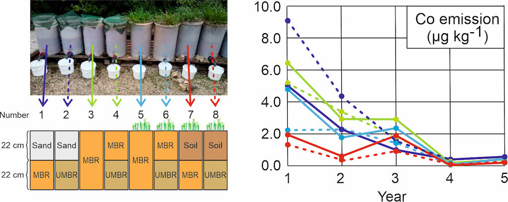
Eight 40-L lysimeters were employed in this study, with varying content including MBR, UMBR, silicate sand, and soil, with a total thickness around 44 cm, as depicted in Figure 1. Lysimeters #1 to #4 remained unvegetated, while lysimeters #5 to #8 underwent a revegetation process. Additionally, a larger 700-L lysimeter (#16) filled with 66 cm (1087 kg) of MBR was subjected to the same revegetation process, aiming to more accurately simulate real MBR storage conditions. This last lysimeter was started a year after the others. To ensure technical and financial feasibility, we prioritized the collection of dense time series data over an extended period, without repetition. Repetition would have necessitated either sparse time series data or a shorter experimental duration. In this context, the consistency in the evolution of various variables over time ensures the validity of the results. Additionally, the comparison of the nine lysimeters further reinforces the robustness of the findings.
The revegetalisation was made with Dactylis glomerata (orchardgrass) and Onobrychis sativa (common sainfoin). The revegetation procedure encompassed the introduction of compost (1% w/w in the top 20 cm layer), N-P-K fertilizer (at an agronomic dose), forest topsoil (1‰ w/w in the upper 22 cm layer), and seeds (agglomerated cocksfoot and common sainfoin). To address trace element requirements, a supplementary supply of soluble manganese was administered at an agronomic dose during the second and third years. Additionally, an annual application of N-P-K fertilizer, matching the initial dose, was conducted. Lysimeters #5, #6, and #16 underwent an initial watering prior to seeding to facilitate seedbed desalination.
During the summer months, a moderate watering was conducted to sustain plants in a vegetative state. This approach facilitated their swift recovery once rainfall resumed, all while preventing runoff. It is noteworthy that the unvegetated lysimeters underwent the same watering regimen.
In year 4 and 5 of the study, a supplement of fresh forest plant litter was introduced onto the topsoil. Lysimeters #5 to #8 received 5 g each, while lysimeter #16 received 15 g. This deliberate addition aimed to foster the colonization of decomposing organisms, as organic matter had accumulated on the surface, forming a cohesive mat.
Notably, the revegetation efforts proved successful for each lysimeter where it was implemented.
2.3. Sample Collection and Analysis
After each rainfall event, drainage samples were systematically collected, acidified with ultrapure acid, and then stored at 2°C. Each year, an annual composite sample was created, proportional to the annual drained volumes of the raw samples. For each sample, measurements of pH, electrical conductivity, and redox potential were recorded. Analyses were performed using ICP-MS at the Eurofins certified laboratory.
Each sample volume was quantified by weighing, allowing for the calculation of the liquid/solid (L/S) ratio in liters per kilogram of residue. This ratio represents the volume of the leachate sample divided by the mass of the residue. Concentration data were expressed in mg L−1, while quantity data were expressed in mg kg−1 by multiplying the concentration by the sample L/S ratio. Cumulative quantities were calculated by summing the quantities of each sample.
3. Results and Discussion
3.1. Effect of Sand or Soil Capping on MBR Emission
This topic was addressed by the results of lysimeters #1 (22 cm of MBR covered by 22 cm of sand), #3 (unvegetated 44 cm of MBR), #5 (vegetated 44 cm of MBR), #7 (22 cm of MBR covered by 22 cm of vegetated soil) and #16 (vegetated 66 cm of MBR).
3.1.1. Hydraulic Properties
The cumulative water input and drainage volumes, expressed in mm of water height (equivalent to L m−2), the drainage/water input ratio and the L/S ratio (litre per kg of MBR) are given on Figure 2 and Table 2.
The drainage/water input ratio was observed to be 99% for the lysimeter #1, indicating that the sand capping greatly limited evaporation. Conversely, lysimeters #3 and #5 exhibited ratios of 67% and 52% respectively, showing that revegetation increased evaporation and consequently reduced drainage. The ratio was lower for the vegetated soil capping (26%), indicating that the soil capping improved water storage or evapotranspiration. The ratio was even lower, by only 20%, for lysimeter #16. Compared to lysimeter #5, the greater thickness of material in lysimeter #16 enabled the augmentation of water storage, thereby increasing the quantity of water available for evaporation.
The potential for leaching of elements towards the depth is higher when the L/S value is high. Here this value decreased with the presence of plant cover and with soil capping (Table 2). The values were nearly identical between lysimeters 5 (vegetated MBR) and 7 (vegetated soil capping), despite the quantity of MBR being half in the latter case, highlighting the effectiveness of soil capping.
3.1.2. pH and Salinity
During the first year of the experiment, the pH levels of leachate remained consistently above 8. Over the subsequent years, there was a gradual decrease, with pH values nearing 7 for lysimeters #1 and #3, and approximately 8 for lysimeters #5 and #16 in the last year. These pH variations align with the changes observed in electrical conductivity, which decreased from the beginning to the end of the experiment (see Figure 3). This indicates a decrease in the alkaline reserve in the soil solution. The latter being in equilibrium with the atmosphere, this explains the decrease in pH. At pHs of the order of 6.5 to 8, most of the potentially toxic elements studied show minimal mobility [26].
The differences among lysimeters can be attributed to the cumulative L/S ratios, as shown in Table 2. Lower ratios indicate a reduced leaching of highly soluble salts, resulting in higher conductivity and pH levels in the leachate at the end of the experiment.
3.1.3. Elements Emission in Leachates
Figure 4 gives the temporal variation of the annual emission per kg of MBR of the elements most likely to pose environmental hazards, such as Na and S due to salinity or sulfation issues for plants and soils, as well as potentially toxic metals or metalloids. Data for all analyzed elements are provided in the supplementary material section. Figure 5 presents the cumulative emission from each lysimeters for all analyzed elements over the entire experimental period (5 years for lysimeters #1 to #7 and 4 year for lysimeter #16).
For most elements in all lysimeters, emission decreased over time. This trend is primarily influenced by the quantity and availability of a soluble stock that is depleting. The slight increase in emissions between year 4 and 5 can likely be attributed to an intense rain event during year 5, where 72 mm of rainfall occurred following 54 mm of cumulative rainfall during the previous four days. This event saturated the lysmeters with water, facilitating diffusive transfer throughout their entire volume and likely temporarily lowering the material redox state, potentially leading to changes in species of the redox-sensitive elements such as As, Fe or V [27].
For most elements, emissions in lysimeters #1, #3 and #5 were higher than those in lysimeters #7, and significantly higher than in lysimeter #16 (Figure 4 and 5). The latter difference can be attributed to the significantly lower L/S ratio in lysimeter #16 compared to other lysimeters. Lysimeter #7 had a L/S ratio similar to that of lysimeter #5 (Table 2), its lower emissions were therefore due to soil caping. Identifying the processes responsible for the better retention of leachable metals would require a dedicated study; however, one hypothesis is the production of non-leachable complexing organic matter in the soil, which could promote the immobilization of metals.
Average annual leachate concentrations are depicted in Figure 6. Consistent with annual emissions, concentrations for most elements were lower for lysimeters #7 and #16 compared to lysimeters #1, #3 and #5, respectively. Ca, Mg and P exhibited higher concentrations in all lysimeters during the final year compared to the first year of the experiment. The increase in Ca and Mg concentrations can be attributed to pH decrease over the course of the experiment, as the solubility of these elements is highly pH-sensitive. The increase in P concentrations is likely due to added fertilizer. Conversely, the concentrations of all other elements were lower in the final year compared to the first year, except for Si, V, Fe, As, Mn and Co in lysimeter #16, which exhibited higher concentration in the final year. As previously mentioned, this can be due to an exceptional waterlogging period during the final year.
There are no international standards for element concentrations in landfill leachates. Existing regulations vary by country and type of filing. Therefore, we compared the observed concentrations with the LD50 toxicity values against Hyelella Azteca [28] (Figure 6). All observed concentrations remained below the LD50 level, except for Cr at the beginning of the experiment. Cd concentration was very close to the LD50 level at the beginning of the experiment. Concentrations of all elements remained under the LD50 values at the end of the experiment, especially knowing that the leachate water is hard (orange stars in Figure 6).
Since leachates have high concentrations of Na that could cause dispersion of clay into the material underlying the landfill, making it impermeable [29], we calculated the SAR (Sodium Absorption Ratio) using the formula
where [Na+], [Ca2+] and [Mg2+] are expressed in mmolc L−1 [30]. SAR and EC values for the first and the final year of the experiment are given in Figure 7. All points are plotted in the area indicating no clay dispersion problems. All leachates, however, remained strongly saline with regard to plant growth.
3.1.4. Effect of Revegetation on MBR or UMBR Emission
The impact of revegetation on emissions was evaluated by comparing lysimeters #3 and #5 (solely MBR) with #4 and #6 (MBR over UMBR), respectively (Figure 8). Overall, revegetation led to an increase in emissions of most metals or metalloids investigated, except for Cr in both MBR-only and MBR/UMBR lysimeters, as well as to a small extent Cu in MBR-only lysimeter and Pb in MBR/UMBR lysimeter. In revegetated lysimeters, it is likely that most metals or metalloids form complexes and can be transported by organic compounds produced by vegetation [33], including As [34]. This process was more intense for lysimeters containing UMBR, probably due to higher mobile metal contents of this material.
Chromium exhibited the opposite trend wih lower emission in vegetated lysimeters. This behavior may be attributed to natural organic matter impeding the oxidation of CrIII to the highly mobile CrVI species [35]. However, further complementary studies would be necessary to fully elucidate this behavior.
3.2. Immobilization of Potentially Toxic Metals by MBR that Has Depolluted Acid Mine Drainage
This topic was addressed by the results of lysimeters #2 (22 cm of UMBR covered by 22 cm of sand), #4 (22 cm of UMBR covered by 22 cm of MBR), #6 (22 cm of UMBR covered by 22 cm of MBR), #8 (22 cm of UMBR covered by 22 cm of vegetated soil) (Figure 1).
3.2.1. Hydraulic Properties
The drainage/water input ratio (Figure 9) as well as the cumulated L/S ratio (Table 3) for lysimeters #2, #4, #6, #8 were almost identical to those observed for lysimeters #1, #3, #5, #7, respectively, leading to the same observation as for the latter lysimeters: sand capping limited evaporation, revegetation increased evaporation and reduced drainage, soil capping improved water storage or evapotranspiration.
Lysimeters with the same coverage have very similar L/S ratios. Revegetation of the MBR cover (lysimeters 5 and 6) reduced the volume of the drains, without reaching the level of a natural topsoil cover (lysimeters 7 and 8).
3.2.2. pH and Salinity
Compared to lysimeters #1, #3, #5 and #7, lysimeters #2, #4, #6 and #8 leachates showed slightly higher pHs and lower ECs at the beginning of the experiment, and almost identical pHs and ECs at the end of the experiment (Figure 3 and Figure 10). This can be related to the fact that the more soluble salts had been already leached in the UMBR material during the acid mine treatment.
3.2.3. Effect of UMBR on Elements Emission in Leachates
Figure 11 gives the temporal variation of the annual emission per kg of MBR or MBR+UMBR of the potentially toxic metals or metalloids. Data for all analyzed elements are provided in the supplementary material section. In lysimeters with UMBR, the behavior of the elements is similar to that observed in lysimeters without UMBR, with an emission which decreases with time reaching very low values in the fifth year, except for vanadium, as previously commented.
Figure 12 illustrates the variation in cumulative emissions between lysimeters with and without UMBR. There was no clear trend in the difference in emissions between lysimeters with and without UMBR. The presence of UMBR led to varying retention and emission patterns for different elements: some elements, such as Al, Cr, and Mo, were more retained, while others, like As, Mn, and Ni, were more emitted. Additionally, the retention or emission of certain elements varied depending on the lysimeter design: sand capping increased emissions for Cd, Co, Cu, Fe, and Ni, whereas soil capping led to higher emissions for Fe, Mn, V, and Zn. Despite these variations, annual average concentrations remained below the LD50 values for all elements except Cr during the first year of the experiment, as previously mentioned.
Interestingly, despite the higher As, Cr, and Zn contents in UMBR, lysimeters with UMBR did not consistently show higher emissions for these elements throughout the experiment. This indicates the effectiveness of UMBR in retaining these elements.
4. Conclusion
Over the course of the 5-year experiment and across all configurations tested – raw, sand capping, soil capping, and revegetation – the pH of the leachates stabilized between 7 and 8, and their salinity gradually decreased. Although the salinity remained significant in the final year, ranging from 3 to 5 mS cm⁻1, the SAR stayed well below the values that could cause clay dispersion and material clogging. Therefore, in all cases, the material remained suitable for the growth of plants compatible with the observed salinity.
Except for V, the emission of potentially toxic elements from the modified bauxite residue (MBR), whether or not it was used to remediate acid mine drainage, rapidly decreased after the first year, reaching low levels. Except for Cr in the first year, the concentrations in the leachates always remained below the LD50 values and reached levels at least one order of magnitude lower than the LD50 by the end of the experiment. Among the different designs studied, sand capping gave less satisfactory results. Revegetation and soil capping also increased emissions, but this increase became insignificant given the low emission levels observed at the end of the experiment.
In conclusion, the spreading of MBR and its revegetation, which prevents dust dispersion, appears to be an environmentally suitable solution for managing bauxite residues like those studied here. However, it is essential to maintain a pH around 7, as acidification of the material below 6.5 could increase the mobility of most potentially toxic elements. Although progressive acidification over time is unlikely in the Mediterranean environment with low deep drainage, this possibility must be monitored in case of spreading in regions with high rainfall.
Supplementary Materials
The following supporting information can be downloaded at the website of this paper posted on Preprints.org, Table S1: Data.
Author Contributions
Conceptualization, P.M. and P.H.; methodology, P.H.; validation, P.M. and P.H.; investigation: P.M., P.H., C.C., A.P.; writing—original draft preparation: P.M.; writing—review and editing, P.M. and P.H.; resources, P.H.; project administration, P.H.; funding acquisition, P.H.
Funding
Funding was provided by the BauGeste (also called Bauxaline Technologies) project (ADEME, Rhône-Mediterranean-Corsica Water Agency (AERMC agreement 2012/0547) and ALTEO) and the Bauxite+ project (ECCOREV-OHM).
Data Availability Statement
Data are given in Supplementary Material.
Conflicts of Interest
The authors declare no conflicts of interest.
References
- Rai, S.; Wasewar, K.; Agnihotri, A. Treatment of alumina refinery waste (red mud) through neutralization techniques: A review. Waste Manag. Res. 2017, 35, 563–580. [Google Scholar] [CrossRef] [PubMed]
- Newson, T.; Dyer, T.; Sharp, S. Effect of structure on the geotechnical properties of bauxite residue. J. Geotech. Geoenviron. Eng. 2006, 132, 143–151. [Google Scholar] [CrossRef]
- Samal, S. Utilization of Red Mud as a Source for Metal Ions—A Review. Mater. 2021, 14, 2211. [Google Scholar] [CrossRef] [PubMed]
- Botelho Junior, A.B.; Espinosa, D.C.R.; Tenório, J.A.S. Characterization of bauxite residue from a press filter system: comparative study and challenges for scandium extraction. Mining Metal. Explor. 2021, 38, 161–176. [Google Scholar] [CrossRef]
- Gu, H.; Wang, N.; Liu, S. Radiological restrictions of using red mud as building material additive. Waste Manag. Res. 2012, 30, 961–965. [Google Scholar] [CrossRef] [PubMed]
- Gu, H.; Wang, N.; Yang, Y.; Zhao, C.; Cui, S. Features of distribution of uranium and thorium in red mud. Physicochem. Problems Mineral Proc. 2017, 53, 110–120. [Google Scholar] [CrossRef]
- Kovács, T.; Sas, Z.; Jobbágy, V.; Csordás, A.; Szeiler, G.; Somlai, J. (2013) Radiological aspects of red mud disaster in Hungary. Acta Geophysica 2013, 61, 1026–1037. [Google Scholar] [CrossRef]
- Liu, Y.; Naidu, R. Hidden values in bauxite residue (red mud): Recovery of metals. Waste Manag. 2014, 34, 2662–2673. [Google Scholar] [CrossRef]
- Klauber, C.; Gräfe, M.; Power, G. Bauxite residue issues: II. options for residue utilization. Hydrometallurgy, 2011, 108, 11–32. [Google Scholar] [CrossRef]
- Verma, A.S. .; Suri, N.M..; Kant, S. Applications of bauxite residue: A mini-review. Waste Manag. Res. 2017, 35, 999–1012. [Google Scholar] [CrossRef]
- Kim, S.Y.; Jun, Y.; Jeon, D.; Oh, J.E. Synthesis of structural binder for red brick production based on red mud and fly ash activated using Ca(OH)2 and Na2CO3. Constr. Build. Mater. 2017, 147, 101–116. [Google Scholar] [CrossRef]
- Rivera, R.M.; Ulenaers, B.; Ounoughene, G.; Binnemans, K.; Van Gerven, T. Extraction of rare earths from bauxite residue (red mud) by dry digestion followed by water leaching. Miner. Eng. 2018, 119, 82–92. [Google Scholar] [CrossRef]
- International Aluminium Institute. Bauxite Residue Management: Best Practice; IAI: London, 2015; pp. 1–31. [Google Scholar]
- Mishra, T.; Pandey, V.C.; Singh, P.; Singh, N.B.; Singh, N. Assessment of phytoremediation potential of native grass species growing on red mud deposits. J. Geochem. Explor. 2017, 182, 206–209. [Google Scholar] [CrossRef]
- Mishra, T.; Singh, N.B.; Singh, N. Restoration of red mud deposits by naturally growing vegetation. Int. J. Phytoremed. 2017, 19, 439–445. [Google Scholar] [CrossRef]
- Kinnarinen, T.; Lubieniecki, B.; Holliday, L.; Helsto, J.-J.; Häkkinen, A. Enabling safe dry cake disposal of bauxite residue by deliquoring and washing with a membrane filter press. Waste Manag. Res. 2015, 33, 258–266. [Google Scholar] [CrossRef]
- Lindsay, W.L. Chemical Equilibria in Soils; John Wiley and Sons Ltd.: Hoboken, 1979. [Google Scholar]
- Barrow, N.J. Possibility of using caustic residue from bauxite for improving the chemical and physical properties of sandy soils. Austral. J. Agric. Res. 1982, 33, 275–285. [Google Scholar] [CrossRef]
- Wong, J.W.C.; Ho, G.E. Use of waste gypsum in the revegetation on red mud deposits : a greenhouse study. Waste Manag. Res. 1993, 11, 249–256. [Google Scholar] [CrossRef]
- Courtney, R.G.; Timpson, J.P. Reclamation of fine fraction bauxite processing residue. red mud) amended with coarse fraction residue and gypsum. Water Air Soil Pollut. 2005, 164, 91–102. [Google Scholar] [CrossRef]
- Pradhan, J.; Das, J.; Das, S.; Thakur, R.S. Adsorption of Phosphate from Aqueous Solution Using Activated Red Mud. J. Colloid Interface Sci. 1998, 204, 169–172. [Google Scholar] [CrossRef]
- Kalin, M.; Fyson, A.; Wheeler, W.N. The chemistry of conventional and alternative treatment systems for the neutralization of acid mine drainage. Sci. Tot. Environ. 2006, 366, 395–408. [Google Scholar] [CrossRef]
- Merdy, P.; Parker, A.; Chen, C.; Hennebert, P. 5-year leaching experiments to evaluate a modified bauxite residue: remediation of sulfidic mine tailings. Environ. Sci. Pollut. Res. 2023, 30, 96486–96498. [Google Scholar] [CrossRef] [PubMed]
- European Communities. Council decision of 19 December 2002 establishing criteria and procedures for the acceptance of waste at landfills pursuant to Article 16 of and Annex II to Directive 1999/31/EC. Official J. Europ. Comm 2023. Available online: https://eur-lex.europa.eu/LexUriServ.do?uri=OJ:L:2003:011:0027:0049:EN:PDF.
- Jacukowicz-Sobala, I.; Ocińsk, i, D.; Kociołek-Balawejder, E. Iron and aluminium oxides containing industrial wastes as adsorbents of heavy metals: Application possibilities and limitations. Waste Manag. Res. 2015, 33, 612–629. [Google Scholar] [CrossRef] [PubMed]
- Cherfouh, R.; Lucas, Y.; Derridj, A.; Merdy, P. Metal speciation in sludges: a tool to evaluate risks of land application and to track heavy metal contamination in sewage network. Environ. Sci. Pollut. Res. 2022, 29, 70396–70407. [Google Scholar] [CrossRef] [PubMed]
- Rinklebe, J.; Antoniadis, V.; Shaheen, S.M. Redox Chemistry of Vanadium in Soils and Sediments: Biogeochemical Factors Governing the Redox-Induced Mobilization of Vanadium in Soils. In Vanadium in Soils and Plants; CRC Press: Boca Raton, Florida, 2022; pp. 95–111. [Google Scholar] [CrossRef]
- Borgmann, U.; Couillard, Y.; Doyle, P.; Dixon, D.G. Toxicity of sixty-three metals and metalloids to Hyalella azteca at two levels of water hardness. Environ. Toxicol. Chem. Int. J. 2005, 24, 641–652. [Google Scholar] [CrossRef]
- Rengasamy, P. Irrigation water quality and soil structural stability: A perspective with some new insights. Agronomy 2018, 8, 72. [Google Scholar] [CrossRef]
- Cherfouh, R.; Lucas, Y.; Derridj, A.; Merdy, P. Long-term.; low technicality sewage sludge amendment and irrigation with treated wastewater under Mediterranean climate: impact on agronomical soil quality. Environ. Sci. Pollut. Res. 2018, 25, 35571–35581. [Google Scholar] [CrossRef]
- Hanson, B.; Grattan, S.R.; Fulton, A. Agricultural salinity and drainage. Water Management Series publication 3375, Davis, 2006. [Google Scholar]
- Wilcox, L.V. Classification and use of irrigation water; U.S.A Dept. Ag. Circ. 696: Washington DC, 1955. [Google Scholar]
- Caporale, A.G.; Violante, A. Chemical processes affecting the mobility of heavy metals and metalloids in soil environments. Cur. Pollut. Rep. 2016, 2, 15–27. [Google Scholar] [CrossRef]
- Dobran, S.; Zagury, G.J. Arsenic speciation and mobilization in CCA-contaminated soils: Influence of organic matter content. Sci. Tot. Environ. 2006, 364, 239–250. [Google Scholar] [CrossRef]
- Pantsar-Kallio, M.; Reinikainen, S.P.; Oksanen, M. Interactions of soil components and their effects on speciation of chromium in soils. Analytica Chimica Acta 2001, 439, 9–17. [Google Scholar] [CrossRef]
Figure 1.
Lysimeters experimental setup. Left: 40-L lysimeters, view and diagram of filling and revegetation; center and right: 700-L lysimeter, shown from the side and from above, respectively.
Figure 1.
Lysimeters experimental setup. Left: 40-L lysimeters, view and diagram of filling and revegetation; center and right: 700-L lysimeter, shown from the side and from above, respectively.
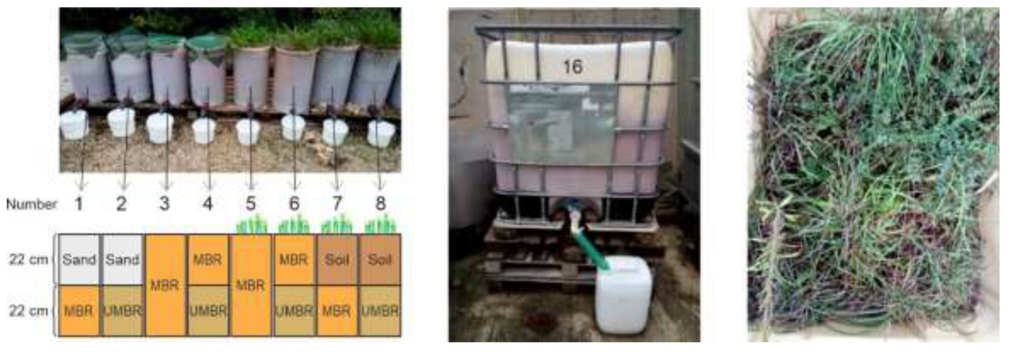
Figure 2.
Water input (rainfall + watering ) (blue columns), drainage (pink columns) and drainage/water input ratio (green columns) of lysimeters #1, #3, #5 and #16.
Figure 2.
Water input (rainfall + watering ) (blue columns), drainage (pink columns) and drainage/water input ratio (green columns) of lysimeters #1, #3, #5 and #16.
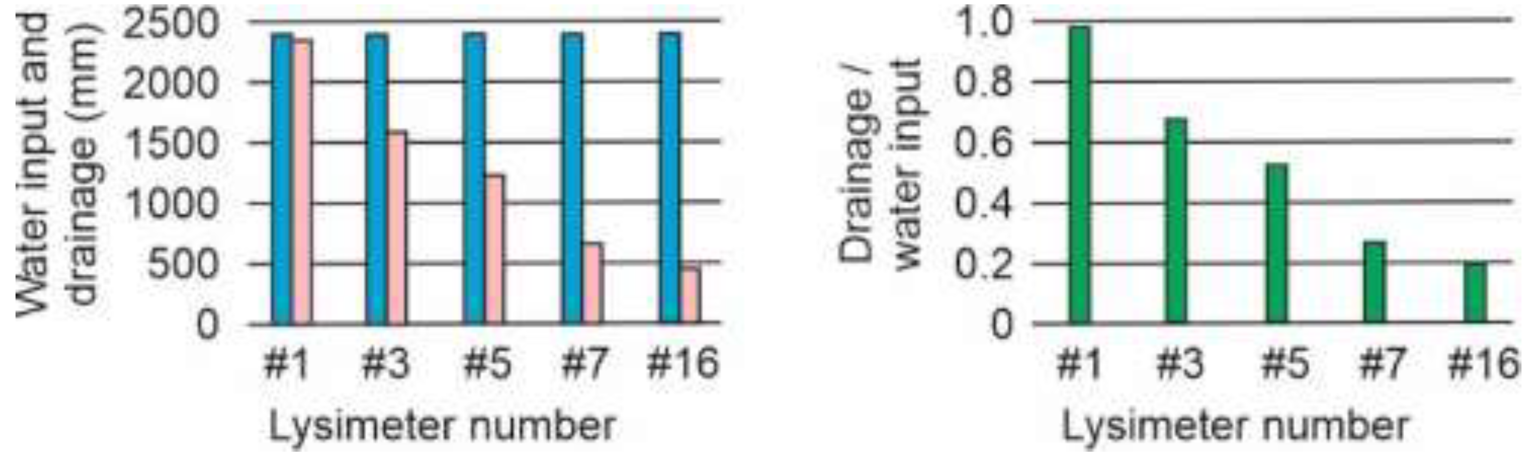
Figure 3.
pH and electrical conductivity (EC) of lysimeters #1, #3, #5, #7 and #16.
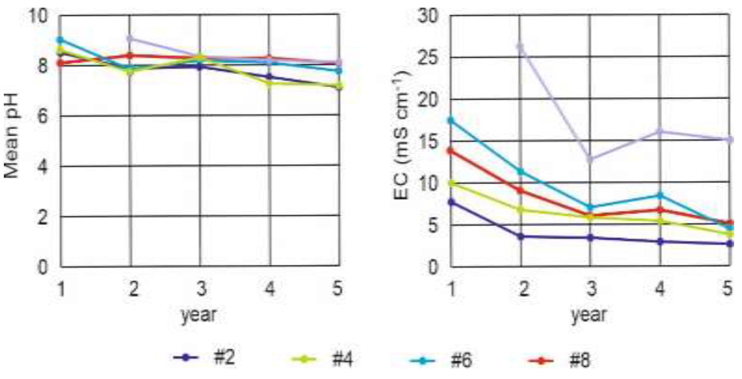
Figure 4.
Variation of emission by leachates over time of some selected elements (Al, Na, S, As, Cd, Co, Cr, Cu, Mo, Ni, Pb, V, Zn) in mg kg−1 of MBR. Sketch of lysimeters, see Figure 1.
Figure 4.
Variation of emission by leachates over time of some selected elements (Al, Na, S, As, Cd, Co, Cr, Cu, Mo, Ni, Pb, V, Zn) in mg kg−1 of MBR. Sketch of lysimeters, see Figure 1.
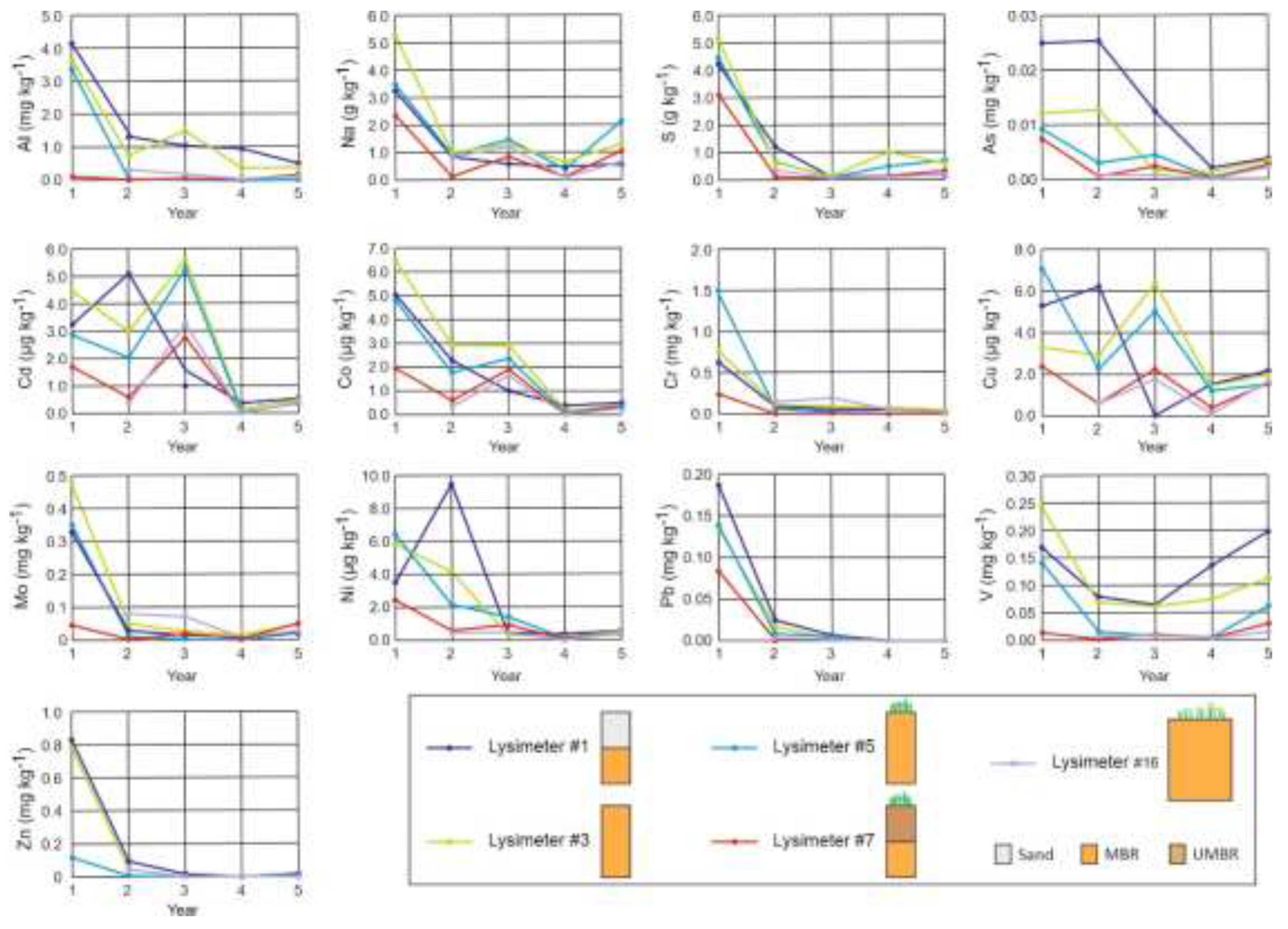
Figure 5.
Cumulated element quantity (mg kg−1 of MBR) emitted by the lysimeters during the 5-years experiment for #1, #3, #5, #7 and the 4-years experiment for #16.
Figure 5.
Cumulated element quantity (mg kg−1 of MBR) emitted by the lysimeters during the 5-years experiment for #1, #3, #5, #7 and the 4-years experiment for #16.
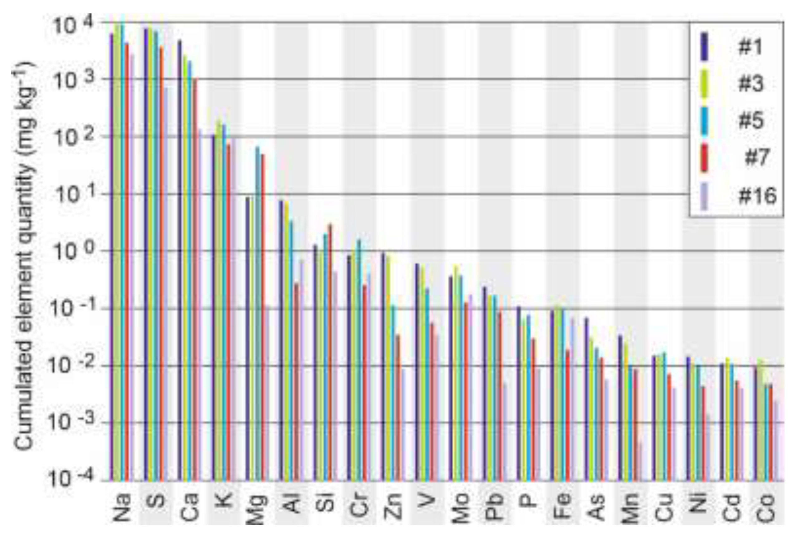
Figure 6.
Concentrations in average annual leachate for the first year and the final year of the experiment. Stars indicate the LD50 concentrations for Hyalella azteca in soft freshwater (hardness 18, red stars) and hard freshwater (hardness 124, orange stars); green stars indicates that the LD50 concentration is over the star value [28].
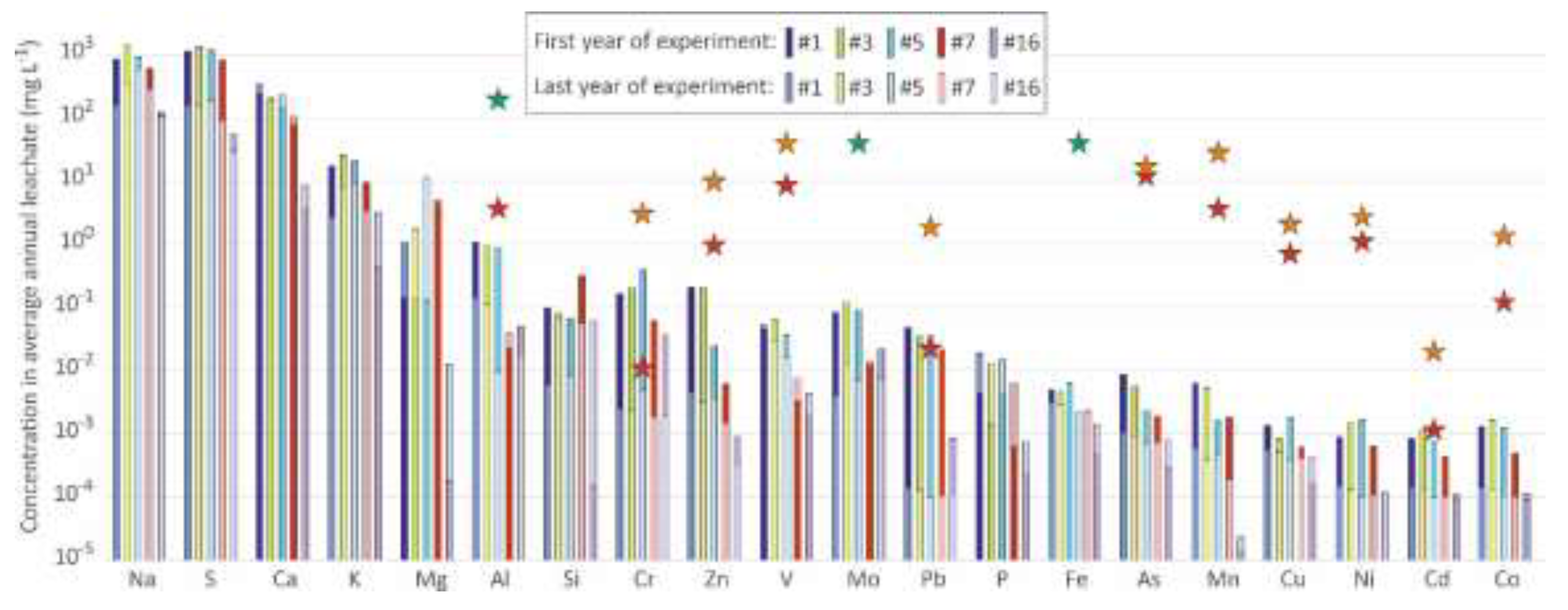
Figure 7.
SAR and electrical conductivity (EC) of lysimeters #1, #3, #5, #7 and #16. Circles and squares give first and final year values, respectively. Areas related to clay dispersion problems were drawn after Hanson et al. [31]. Hatched area represents high and very high salinity with regard to plant growth [32].
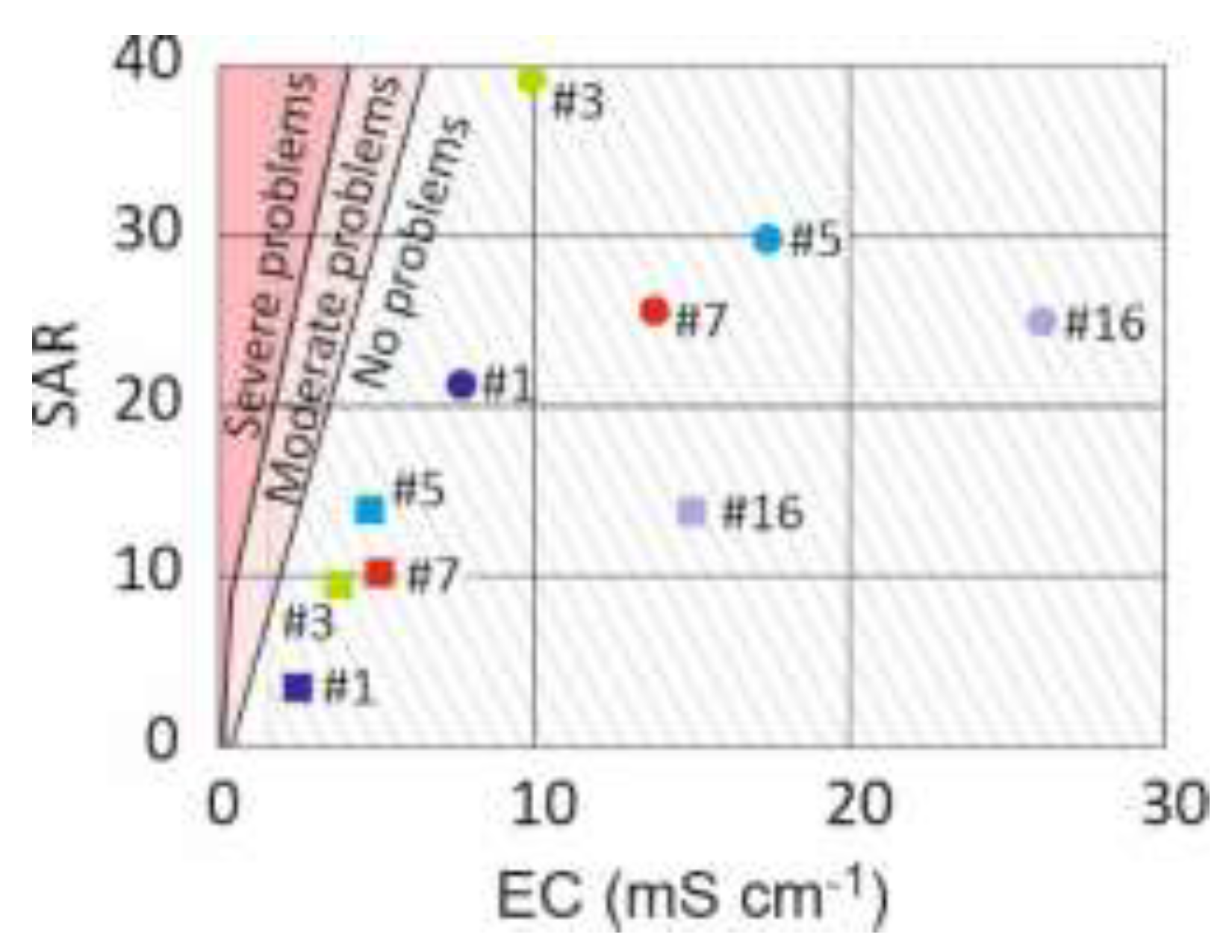
Figure 8.
Emission from a vegetated lysimeter (#5 and #6) as a % of the corresponding non-vegetated lysimeter (#3 and #4, respectively). Cumulative emissions during the 5 years of experimentation.
Figure 8.
Emission from a vegetated lysimeter (#5 and #6) as a % of the corresponding non-vegetated lysimeter (#3 and #4, respectively). Cumulative emissions during the 5 years of experimentation.
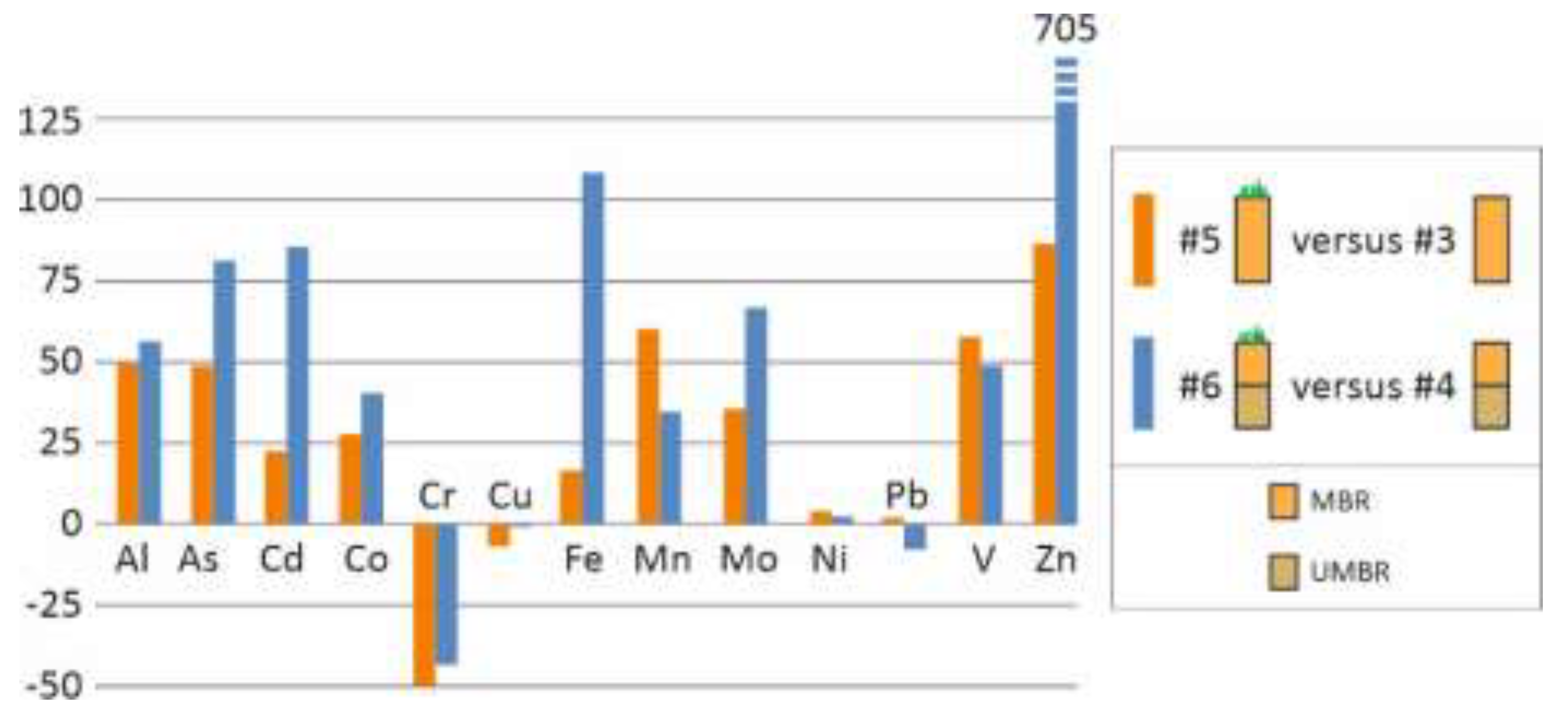
Figure 9.
Water input (rainfall + watering ) (blue columns), drainage (pink columns) and drainage/water input ratio (green columns) of lysimeters #2, #4, #6 and #8.
Figure 9.
Water input (rainfall + watering ) (blue columns), drainage (pink columns) and drainage/water input ratio (green columns) of lysimeters #2, #4, #6 and #8.
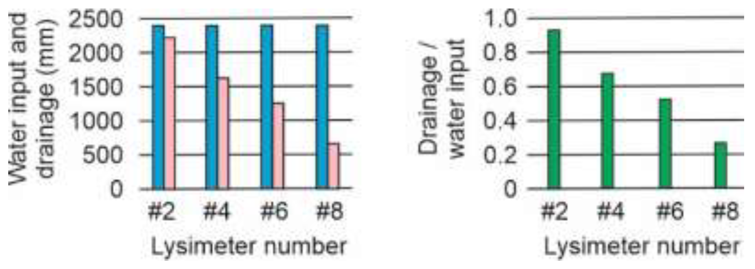
Figure 10.
pH and electrical conductivity (EC) of lysimeters #2, #4, #6 and #8.
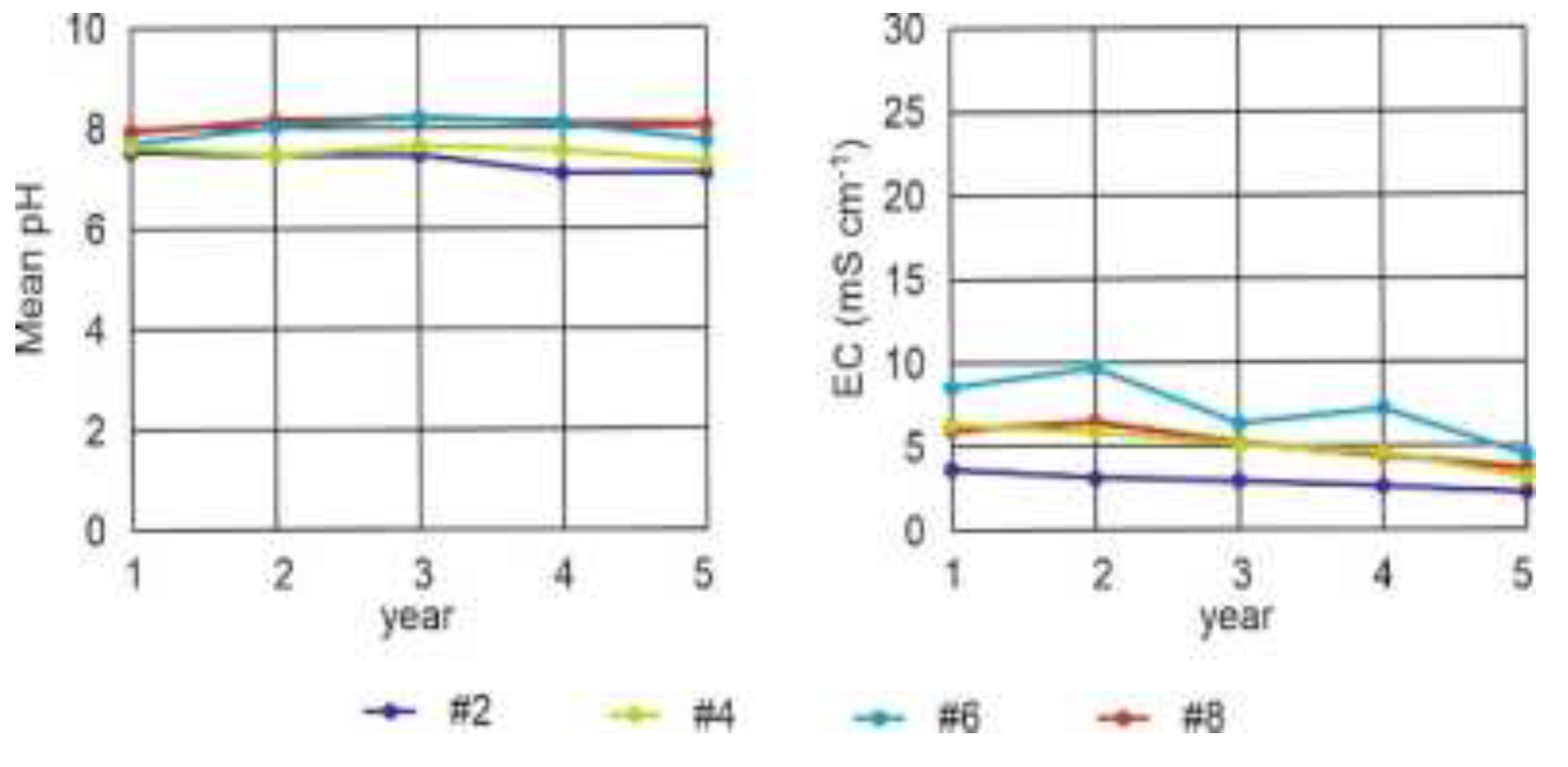
Figure 11.
Variation of emission by leachates over time of potentially toxic elements (Al, As, Cd, Co, Cr, Cu, Mo, Ni, Pb, V, Zn) in mg kg−1 of (MBR+UMBR). Sketch of lysimeters, see Figure 1.
Figure 11.
Variation of emission by leachates over time of potentially toxic elements (Al, As, Cd, Co, Cr, Cu, Mo, Ni, Pb, V, Zn) in mg kg−1 of (MBR+UMBR). Sketch of lysimeters, see Figure 1.
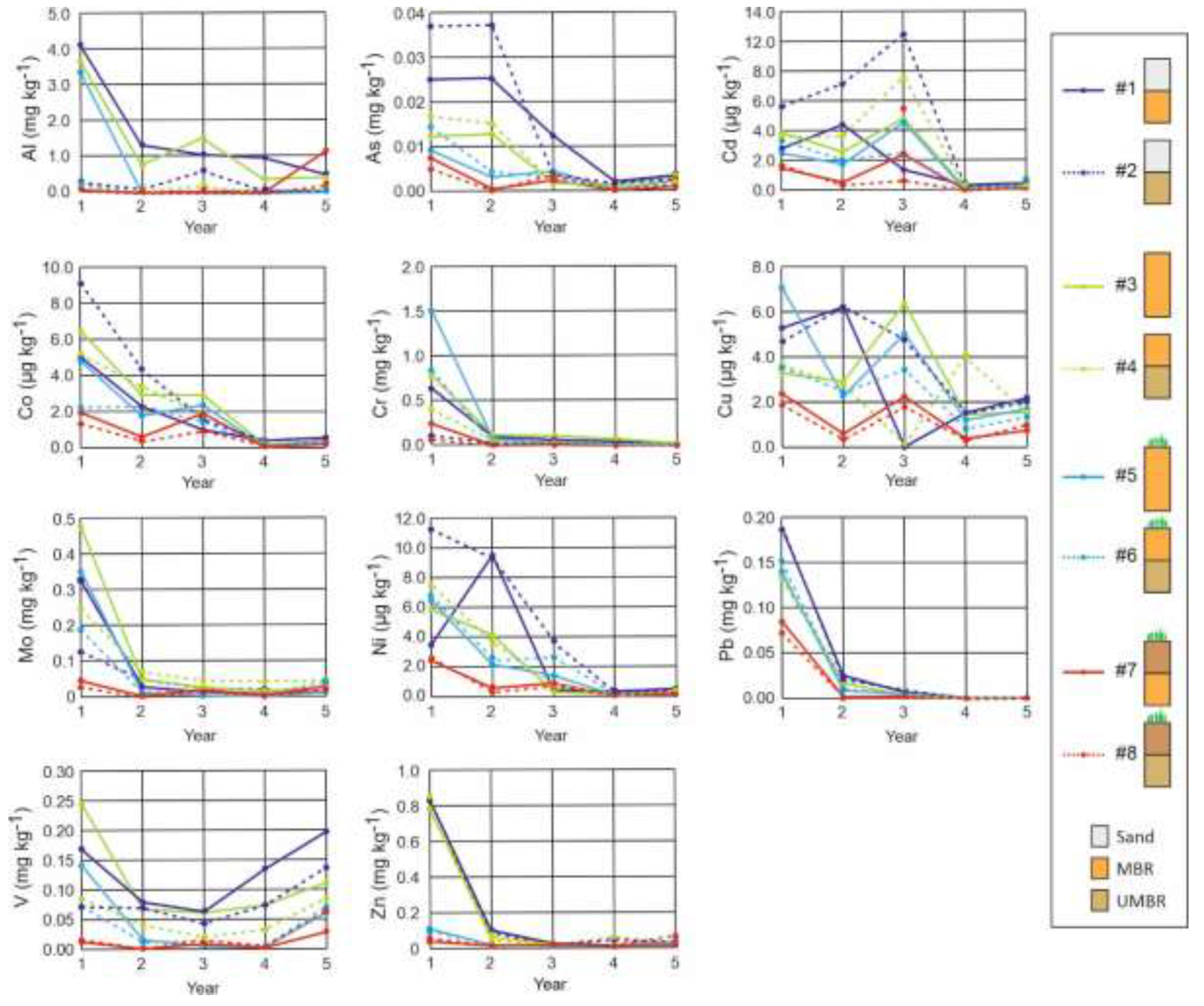
Figure 12.
Emission from lysimeter with UMBR as a % of the corresponding lysimeter without UMBR. Cumulative emissions during the 5 years of experimentation.
Figure 12.
Emission from lysimeter with UMBR as a % of the corresponding lysimeter without UMBR. Cumulative emissions during the 5 years of experimentation.
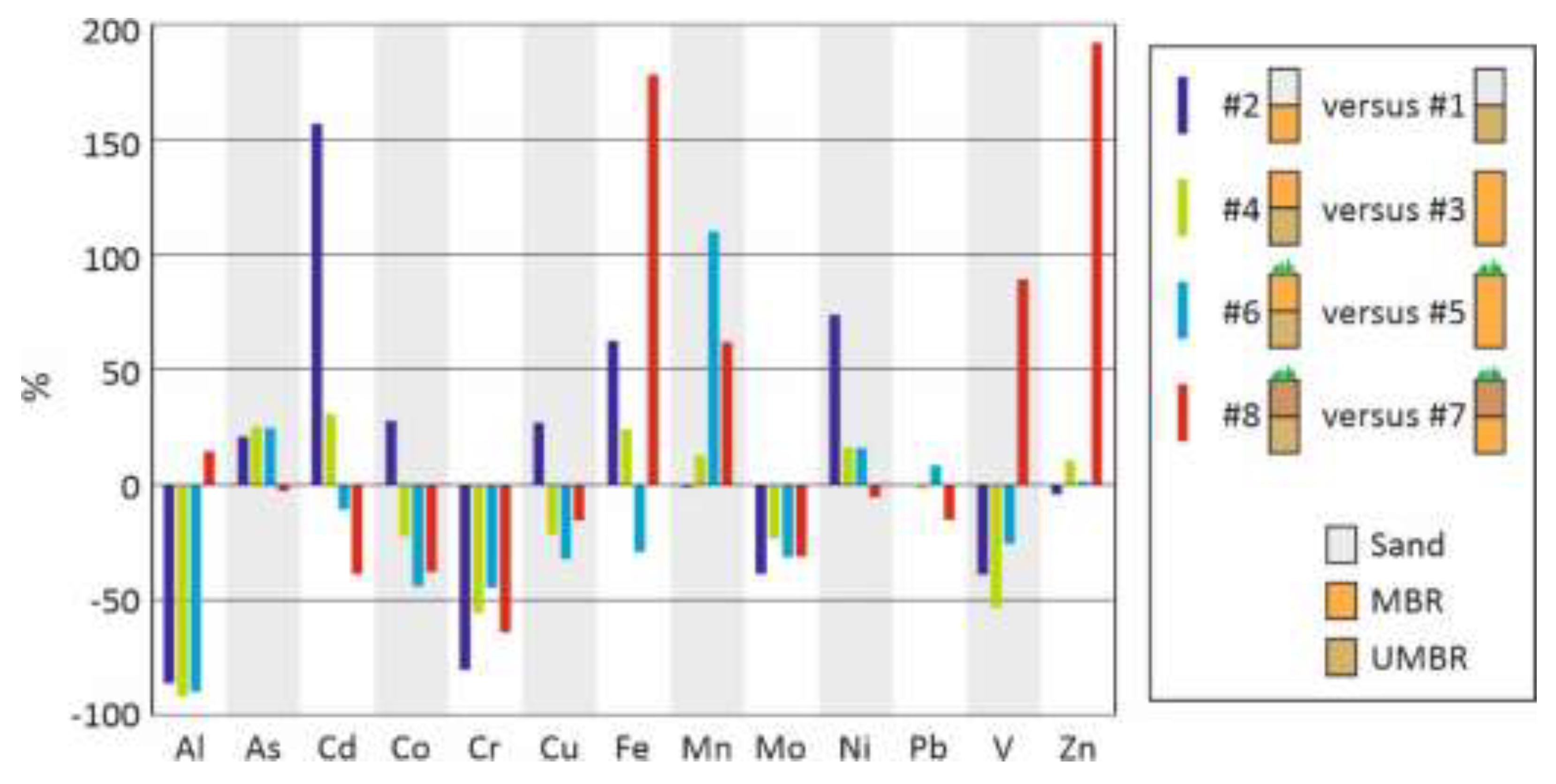

Table 1.
Usual range of major and potentially toxic elements in the Bauxaline® and composition of the Bauxaline® used in the present study. IWSF and NHWSF: concentration limits of leachable elements for admission to Inert waste storage facility and Non-hazardous waste storage facility, respectively.
| Major elements (%) | Trace elements (ppm) | |||||||
| Usual range | Present study | Usual range | Present study | IWSF | NHWSF | |||
| Al | 1.6 – 8.1 | 7.9 | As | 10 - 200 | 18 | 0.5 | 2 | |
| Ca | 1.4 – 4.8 | 4.3 | Cd | <0.5 - 10 | 0.8 | 0.04 | 1 | |
| Fe | 21.0 – 38.0 | 32.2 | Co | 1 – 75 | 35 | |||
| Na | 1.5 – 3.0 | 3.0 | Cr | 200 - 2000 | 1638 | 0.5 | 10 | |
| Si | 0.9 – 3.9 | 3.3 | Hg | <1.5 – 2 | 0.2 | |||
| Ti | 1.8 – 5.4 | 6.0 | Ni | 5 – 50 | 18 | 0.4 | 10 | |
| Pb | 10 - 100 | 42 | 0.5 | 10 | ||||
| Se | <1.5 - 50 | <6 | 0.1 | 0.5 | ||||
| V | 200 - 1500 | 968 | ||||||
| Zn | <20 - 500 | 115 | 4 | 50 | ||||
Table 2.
Cumulated L/S ratio (L kg−1 of MBR) of lysimeters #1, #3, #5, #7 and #16.
| #1 | #3 | #5 | #7 | #16 | |
| Year 1 | 2.68 | 1.16 | 0.88 | 1.02 | - |
| Year 1 to 2 | 3.85 | 1.45 | 1.02 | 1.08 | 0.09 |
| Year 1 to 3 | 5.12 | 1.85 | 1.33 | 1.60 | 0.26 |
| Year 1 to 4 | 6.67 | 2.22 | 1.46 | 1.72 | 0.30 |
| Year 1 to 5 | 8.89 | 2.99 | 2.31 | 2.48 | 0.46 |
Table 3.
Cumulated L/S ratio (L kg−1 of MBR) of lysimeters #2, #4, #6 and #8.
| #2 | #4 | #6 | #8 | |
| Year 1 | 2.55 | 2.39 | 2.20 | 0.85 |
| Year 1 to 2 | 3.68 | 2.99 | 2.53 | 0.89 |
| Year 1 to 3 | 4.95 | 3.74 | 3.19 | 1.40 |
| Year 1 to 4 | 6.38 | 4.55 | 3.37 | 1.51 |
| Year 1 to 5 | 8.39 | 6.15 | 4.76 | 2.54 |
Disclaimer/Publisher’s Note: The statements, opinions and data contained in all publications are solely those of the individual author(s) and contributor(s) and not of MDPI and/or the editor(s). MDPI and/or the editor(s) disclaim responsibility for any injury to people or property resulting from any ideas, methods, instructions or products referred to in the content. |
© 2024 by the authors. Licensee MDPI, Basel, Switzerland. This article is an open access article distributed under the terms and conditions of the Creative Commons Attribution (CC BY) license (http://creativecommons.org/licenses/by/4.0/).
Copyright: This open access article is published under a Creative Commons CC BY 4.0 license, which permit the free download, distribution, and reuse, provided that the author and preprint are cited in any reuse.


