

Submitted:
22 October 2024
Posted:
23 October 2024
You are already at the latest version
Abstract
This study presents the design and analysis of a proportional electromagnet used in electro-pneumatic brake systems for heavy vehicles. The solenoid was designed using a traditional method and its static and dynamic characteristics were investigated both theoretically and experimentally. ANSYS Maxwell was employed for theoretical static analysis, focusing on the effects of geometric dimension parameters in the fixed and moving pole contact region on the Force-Displacement characteristics. Optimal dimensions for proportionality were determined under suitable operating conditions. The static analysis results provided magnetization curve data, which were used to create look-up tables for a dynamic model in MATLAB-Simulink. Following static analysis, a prototype electromagnet was manufactured and tested. The solenoid achieved a constant magnetic force of 45 ± 3N with a current of 1.3A over a working range of 1-3 mm. The dynamic model, incorporating data from ANSYS, yielded results that closely matched experimental findings.
Keywords:
electromagnetic
; actuator
; FEM
; proportional solenoid actuator
; constant force characteristics
; proportional solenoid valve
; solenoid
; dynamic model
; look-up table
; optimization
1. Introduction
Electromechanical actuators are one of the most important elements of mechatronic systems and are used in different applications as the final control element that converts electrical signal to mechanical motion. Depending on the developments in electronic technology, electromechanical proportional valves find a widespread use in the industry from automotive to hydraulic and pneumatic systems, from process control applications to home electronics. It can be made proportional by making some changes in the geometry of on-off type solenoids. In the literature, the effects of geometry on force characteristics have been studied [1-6]. There are also studies on the dynamic system model in the literature [7,8]. However, in these studies, the solution time is prolonged due to the large number of nonlinear equations. A new method using look-up tables for the dynamic system of the solenoid has been investigated by Topcu et al. [9]. The simulation run times of the simplified model is about 50% less than those of the traditional model which contains nonlinear effects while the accuracy of the solutions remains the same. In this study, a Look-Up Table data was obtained by taking the Air gap-Current-Force data according to the analysis obtained from the ANSYS-Maxwell static model.
2. Materials and Methods
In this study, first of all, a flat-faced piston-type electromagnet that provides 50N force under certain limitations for an electromechanical pneumatic brake valve is pre-designed. Then, by changing the geometric parameters in the literature [3], a proportional solenoid design that provides sufficient constant force in the desired working region has been made. By following the classical electromagnet design steps [10], the dimensions (Figure 1) of the solenoid providing the desired force according to the size limitations were obtained as shown in Table 1.
The magnet force of the pre-designed electromagnet is expressed as follows.
As seen from Eq. 1; the magnet force varies directly with the square of the applied current and is inversely proportional to the amount of the result in mechanical movement that results. Accordingly, the magnetic force is a non-linear function of the current and displacement. The displacement-magnet force characteristics for a constant current for this electromagnet were obtained using the magnetic finite element method in the Maxwell module of the ANSYS program. It is known that in the on-off type solenoids, the magnet force is high in the range where the distance between the fixed pole and the moving pole is very small, whereas the magnet attraction force decreases suddenly as the distance increases. Therefore, a nonlinear characteristic is seen in the force curve corresponding to the change in distance for a given current [11,12]. This type of solenoid is suitable for on-off type valves but not for proportional valve. As seen in Figure (2), in proportional solenoids, it is possible to provide a magnet force proportional to the current change by creating a region that gives a constant force in a certain operating range between the position and the force. It is possible to obtain a proportional solenoid by changing the geometric structure of the classical on-off type solenoid, and there are various studies and applications on this subject in the literature [3,13]. In this study, a proportional solenoid design was made using ANSYS Maxwell solenoid model and defined new geometric dimensions. As can be seen from Eq.1, magnet force, in standard solenoids is a nonlinear function of current and displacement. On the other hand, in proportional solenoids, the magnetic force can be expressed as independent of the amount of movement in the working region, only depending on the current change. Generally, in solenoid-controlled valves, the moving element works against a spring force, and from the balance of these forces can be expressed as:
where is magnetic force, is the spring counter force, is the spring constant, is the displacement and is the exciting current. The function is linear and can be controlled by varying the current. As can be seen from Figure 2, proportionality can be established between the position of the moving element and the current passing through the coil. Because of the linearity of the function, solenoids of this type are called proportional solenoids (linear solenoids). The force-displacement characteristic of the proportional solenoid against a certain current value is as given in Figure 2. Here, the range in which the force remains constant is defined as the proportional operating region.
In this study, a change was made in the geometry of the fixed pole opposite the moving pole (Figure 3). In this way, some of the magnetic flux is provided to flow over the iron material at low air gap distance and excessive force increase is prevented.
2.1. Optimization of Solenoid Taper Section Geometry
Different methods have been used to linearize the current-force characteristic of the solenoid [14]. In this article, force characteristics for different situations are investigated by adding a conical geometry to the fixed pole. As shown in Figure 3, the parameters added to the radius of the fixed pole, known as taper section width , taper section length , taper section tip width and taper height are as variable parameters. The effects of , and values of these parameters on the force-displacement characteristics of the solenoid were analyzed in computer environment. Two out of these three parameters were analyzed by changing the constant and the other within the specified range. As seen in Figure 4, the effect of each parameter change on the solenoid characteristic is different.
Therefore, these different parameter values of the solenoid geometry should be selected by the desired static force characteristic. In order to obtain a constant attraction force independent of displacement under a certain current in the working region, the parameters , and are chosen as design variables and force characteristics can be obtained for their different combinations. Appropriate dimensions can be obtained by optimizing using the least squares method as shown in Figure 5.
The objective function has been defined as:
In Eq. 3; is the number of force characteristics to be calculated, is the intended force magnitude, is the calculated magnetic force values at different positions of the moving pole. parameter is from 2mm to 4mm in 0.25mm steps; parameter is from 0.5mm to 2.5mm in 0.9mm steps and also at =0.1mm and =0.3mm; By increasing the parameter from 0.5mm to 5mm by 1mm steps, the air gap was increased by 0.5mm from 1mm to 3.5mm, and 2268 analyzes were carried out and the most appropriate results are given in Figure 6.
2.2. Finite Element Model and Experimental Setup
According to this optimization, it has been determined that the parameters =3.0 mm, =0.2 mm, =2.5mm are the dimension combination with the lowest value of the objective function for the design. Finite element analysis is performed for this dimension, and magnetic field strength and magnetic flux density analyzes are given in Figure 7a and Figure 7b. As seen in the figure, the largest flux density is in the conical part of the solenoid and is in the order of 0.9 Tesla.
The experimental setup designed for the experimental analysis of static and dynamic characteristics is shown in Figure 8. The brand and model of the load cell used for force measurement in this setup; Puls Elektronik is the STA Series Load Cell and the model with a maximum capacity of 50kg has been selected. Panasonic Laser Sensor HL-G105-A-C5 position sensor was used to measure the position of the moving core of the solenoid in the experimental setup, its resolution is 1.5µm, the measuring range is 10mm, the sampling time is 200µs, 500µs, 1ms, 2ms and a desired value can be selected from the menu. The current driver circuit is driven with 15V DC electrical voltage, two LM741 opamps are used. Proxxon brand and KT70 model screw shaft mechanism module is used for linear motion; The stroke in the X direction is 134 mm, and the stroke in the Y direction is 46 mm. Feedback brand power supply providing ±15V DC electrical voltage is used to feed the circuit.
2.3. Dynamic Model of the Solenoid
In Figure 9, the dynamic model of the proportional solenoid whose static characteristics were obtained using ANSYS/Maxwell has been shown. The physical structure of the solenoid, whose dynamic analysis is performed, consists of an electrical, magnet and mechanical subsystems [11].
2.3.1. Electrical Subsystem
The coil, which forms the electrical part of the solenoid, is ideally modeled as a series-connected resistor and an inductance element.
where, dL/dx is the motion dependent change of inductance, the magnetic flux is a function of current and displacement in the form of Φ(i,x).
therefore
Numerical solution of this equation is done by either inductance or magnet flux change method.
2.3.2. Magnetic Subsystem
The magnet subsystem consists of a coil of copper conductor wire and a fixed pole and a moving pole of the electromagnet material in which this coil is placed. A magnet attraction force occurs as a result of the magnet energy change occurring in this subsystem. The magnet attraction force is expressed as Eq. 4 depending on the inductance change and this equation is used to calculate the force in the inductance method.
The magnetic attraction force depending on the magnet flux change;
is expressed as and this equation is used in the magnet flux method.
2.3.3. Mechanic Subsystem
The mechanical subsystem is modeled as mass (m), spring (k) and damper (b). The equation of motion for the mechanic subsystem can be obtained using Newton’s equations.
2.3.4. Solving the Dynamic Equations
Since the equations for each subsystem of the solenoid and describing the whole system are not linear, their analytical solutions are very difficult to solve. In this study, computer aided numerical solution was applied using MATLAB/Simulink. The Simulink model for the solution of dynamic equations can be constructed using two methods [9,12].
In the first method, besides the basic equation of the three subsystems, the reluctance and permeability equations of the magnet circuit are used. This equation contains complex algebraic expressions that depend on the geometry of the magnet circuit. In addition, algebraic expressions in the Simulink model extend the solution time and often make it insoluble.
Another method is to use tables of reluctance and magnet flux values due to electric current and displacement. These tables, which are prepared through experimental, static analysis or calculations, can be used as a Look-up Table function in the Simulink model. In this way, the solutions are faster and the simulation results are closer to the real results [9].
In this study, Look-Up Table method was used to solve dynamic behavior equations in Simulink environment. The data in the Look-Up Table were obtained from the solution of the magnet circuit with the ANSYS/Maxwell finite element program and shown in Figure 10.
From the Maxwell SEM analysis results, matrices that give the values of force, and magnetic flux linkage were created versus current-air gap values. The calculated magnetic force data versus the current, displacement, values in the Maxwell model are defined in the block named “Lookup1, ” in the Simulink model (Figure 9). On the other hand, a MATLAB program was prepared that gives the magnetic flux linkage, versus the current-air gap. The obtained current data versus the air gap, and flux linkage, values in the MATLAB program are defined in the block named “Lookup 2, ” in the Simulink model (Figure 9).
The electrical subsystem of the dynamic model seen in Figure 9 is prepared using the expression given in Eq. 5. The mechanical subsystem is formed using the expression given in Eq. 7. Proportional solenoids have moving and fixed poles. When current is applied to the coil, the moving element completes its movement in the air gap in three stages: i) Starting motion (< , ), ii) Moment of motion (> ,) iii) End of motion (). These stages are defined in the Conditions subsystem of the dynamic model.
Solenoid with resistance , input voltage is applied in the model. It is assumed that the movable element moves . Pretension force, spring coefficient, and viscous friction coefficient are neglected.
The simulation results of the dynamic model given in Figure 9 are shown in Figure 11. As seen in these graphs, the moving element completes its motion in about 15ms. According to the simulation results, the response rate for 1.6 A current, that is, the time the moving element completes its movement, is 15 ms and the time to settle to the final current value is 120 ms. It is seen that the current curve makes a pit during the completion of the movement. In this type of electromechanical system, the time that the current pit is used to determine the response time [15].
The dynamic test results were obtained according to the step input signal and a certain current versus voltage signal was applied as input in the experiments. A typical step response curve is given in Figure 11. According to the dynamic test results given in Figure 11, the pitting time of the measured current is 15 ms, that is, the time to complete the movement of the moving element took 15 ms. When the movement was completed, the current increased and reached its final value in 120 ms.
3. Results
In this study, the design and analysis of a proportional solenoid constituting the pilot stage of the electro-pneumatic brake valve used in heavy vehicles was carried out. The design criteria were taken from a system used in the application and a standard on-off type solenoid design was carried out during the preliminary design phase.
By changing the geometry of the pre-designed on-off type solenoid magnet circuit, a solenoid design that provides proportional characteristics has been obtained. For this, the diameter of the fixed pole forming the magnet circuit has been increased compared to the moving pole and a conical projection in which the moving pole operates has been formed. In this way, the magnet flux path is deflected in small air gaps and a permanent magnet force is obtained in a certain operating range. It has made the magnetic force independent of the air gap in a certain working region and has made it proportional only to the current change.
It is not possible to write a direct mathematical relationship between the solenoid magnet circuit and the force-current variation. Therefore, the optimization of the geometry providing the proportional characteristics could be performed with the help of the ANSYS/Maxwell program based on the finite element method. The analysis program was run more than 2000 times and the proportional solenoid geometry providing constant magnetic force reaching the design criteria was obtained.
As a result of the analyzes made for the ANSYS/Maxwell model of the solenoid, whose design has been completed, it is shown that the force-air gap characteristic provides the desired 42 N force in the range of 1-3 mm with a current of 1.3 A (Figure 12 a).
The force graph of the optimized solenoid for different currents at different positions is given in Figure 12-b. As can be seen from Figure 12-b, the flow force curves were superimposed on each other when the air gap was between 1.00 mm-3.00 mm. However, for values outside 1.0 -3.0 mm of the air gap (0.5 and 3.5 mm for this graph), the current-force curves are scattered up and down. In other words, it can be interpreted that this region corresponds to the uncontrollable region for the proportional solenoid.
For each different current value, different forces were obtained regardless of the displacement. In this way, the force function from the form is dependent only on the current, taking the form ignoring the displacement term .
When the on-off type solenoid valve with the same geometry is compared with the designed proportional valve: the on-off type solenoid provides a relatively high magnet force such as 70 Newton’s in low air gaps and drops to the order of 10 Newton’s in wide air gaps; whereas the designed proportional solenoid provides a magnet force of around 45 Newton’s at maximum current, but it can maintain this value throughout the movement.
The force characteristic of the designed proportional solenoid is only a function of the current, independent of the displacement. It has been proven that the force increases approximately linearly with current. Thus, it has become possible to drive and control the proportional solenoid with current.
The response time of the proportional solenoid from the dynamic response curve was found to be about 15ms as seen in Figure 11.
4. Discussion
A sufficient agreement has been obtained between the simulation and experimental results of the dynamic characteristics, and it has been determined that the solenoid has a response time of about 15 ms. This response time, on the other hand, was found to be in a suitable value for the targeted result. In addition, this response time has been found to be sufficient especially in heavy vehicle commercial vehicle braking systems where this type of proportional solenoid valves is used. A test setup suitable for determining the static and dynamic characteristics of the proportional solenoid was designed and manufactured.
As a result, a proportional solenoid design and prototype production targeted within the scope of the project was carried out, and it was seen that this solenoid also met the design criteria. In addition, it has been determined that the theoretical and experimental results obtained as a result of the analyzes and experiments are reasonably compatible for this study area.
Author Contributions
Conceptualization, E.D.; methodology, E.D.; software, E.D. and G.Ş.; validation, E.D.; formal analysis, E.D. and G.Ş.; investigation, E.D.; resources, E.D. and G.Ş.; data curation, E.D. and G.Ş.; writing—original draft preparation, E.D.; writing—review and editing, E.D. and G.Ş.; visualization, E.D.; supervision, G.Ş.; project administration, G.Ş.; funding acquisition, G.Ş. All authors have read and agreed to the published version of the manuscript.
Funding
This research was funded by MINISTRY OF SCIENCE, INDUSTRY AND TECHNOLOGY OF TÜRKİYE, grant number 0700. STZ. 2014.
Informed Consent Statement
Informed consent was obtained from all subjects involved in the study.
Conflicts of Interest
The authors declare no conflicts of interest.
References
- Vogel, O.; Ulm, J. Theory of proportional solenoids and magnetic force calculation using Comsol multiphysics. In Proceedings of the 2011 COMSOL Conference, Stuttgart, Germany; 2011. [Google Scholar]
- Lequesne, B.P. Finite-element analysis of a constant-force solenoid for fluid flow control. IEEE Trans. Ind. Appl. 1988, 24, 574–581. [Google Scholar] [CrossRef]
- Yun, S.-N.; Ham, Y.-B.; Shin, H.-B. Proportional fuel flow control valve for diesel vehicle. In Proceedings of the 2008 International Conference on Control, Automation and Systems, IEEE, Seoul, Korea; 2008; pp. 94–98. [Google Scholar]
- Douglas, J.F. Solenoid plunger magnet with nearly constant force. IEEE Trans. Appl. Ind. 1963, 82, 331–334. [Google Scholar] [CrossRef]
- Yun, S.-N.; Ham, Y.-B.; Park, J.-H. New approach to design control cone for electro-magnetic proportional solenoid actuator. In Proceedings of the 2012 IEEE/ASME International Conference on Advanced Intelligent Mechatronics (AIM), IEEE, Kaohsiung, Taiwan; 2012; pp. 982–987. [Google Scholar]
- Yun, S.-N.; Ham, Y.-B.; Park, J.-H. Attraction force improvement strategy of a proportional solenoid actuator for hydraulic pressure control valve. In Proceedings of the 2012 12th International Conference on Control, Automation and Systems, IEEE, Jeju, South Korea; 2012; pp. 1123–1127. [Google Scholar]
- Richer, E.; Hurmuzlu, Y. A high performance pneumatic force actuator system: Part i—nonlinear mathematical model. J. Dyn. Syst. Meas. Control 2000, 122, 416–425. [Google Scholar] [CrossRef]
- Szente, V.; Vad, J.; Lorant, G.; Fries, A. Computational and experimental investigation on dynamics of electric braking systems. In Proceedings of the 7th Scandinavian International Conference on Fluid Power, Citeseer, Tampere, Finland, 2001; Vol. 1; pp. 263–275. [Google Scholar]
- Topçu, E.E.; Kamış, Z.; Yüksel, İ. Simplified numerical solution of electromechanical systems by look-up tables. Mechatronics 2008, 18, 559–565. [Google Scholar] [CrossRef]
- Roters, H.C. Electromagnetic Devices; J. Wiley & Sons, Inc.: New York, NY, USA, 1941. [Google Scholar]
- Sefkat, G. Investigating static and dynamic characteristics of electromechanical actuators (ema) with MATLAB GUIs. Comput. Appl. Eng. Educ. 2010, 18, 383–396. [Google Scholar] [CrossRef]
- Sefkat, G. The design optimization of the electromechanical actuator. Struct. Multidiscip. Optim. 2009, 37, 635–644. [Google Scholar] [CrossRef]
- Park, S.; Lee, J.; Yoo, J.; Kim, D.; Park, K. Effects of design and operating parameters on the static and dynamic performance of an electromagnetic valve actuator. Proc. Inst. Mech. Eng. Part D J. Automob. Eng. 2003, 217, 193–201. [Google Scholar] [CrossRef]
- Meng, F.; Chen, H.; Liu, H.; Han, B.; Nie, X. The optimization of a proportional solenoid valve design for heavy vehicle active suspension system. Int. J. Veh. Des. 2015, 68, 180–200. [Google Scholar] [CrossRef]
- Şefkat, G. Bir elektromekanik aygıtın statik ve dinamik karakteristiğinin araştırılması. Pamukkale Univ. Mühendis. Bilim. Derg. 2002, 8, 273–282. [Google Scholar]
Figure 1.
Solenoid cross-sectional view and dimensions
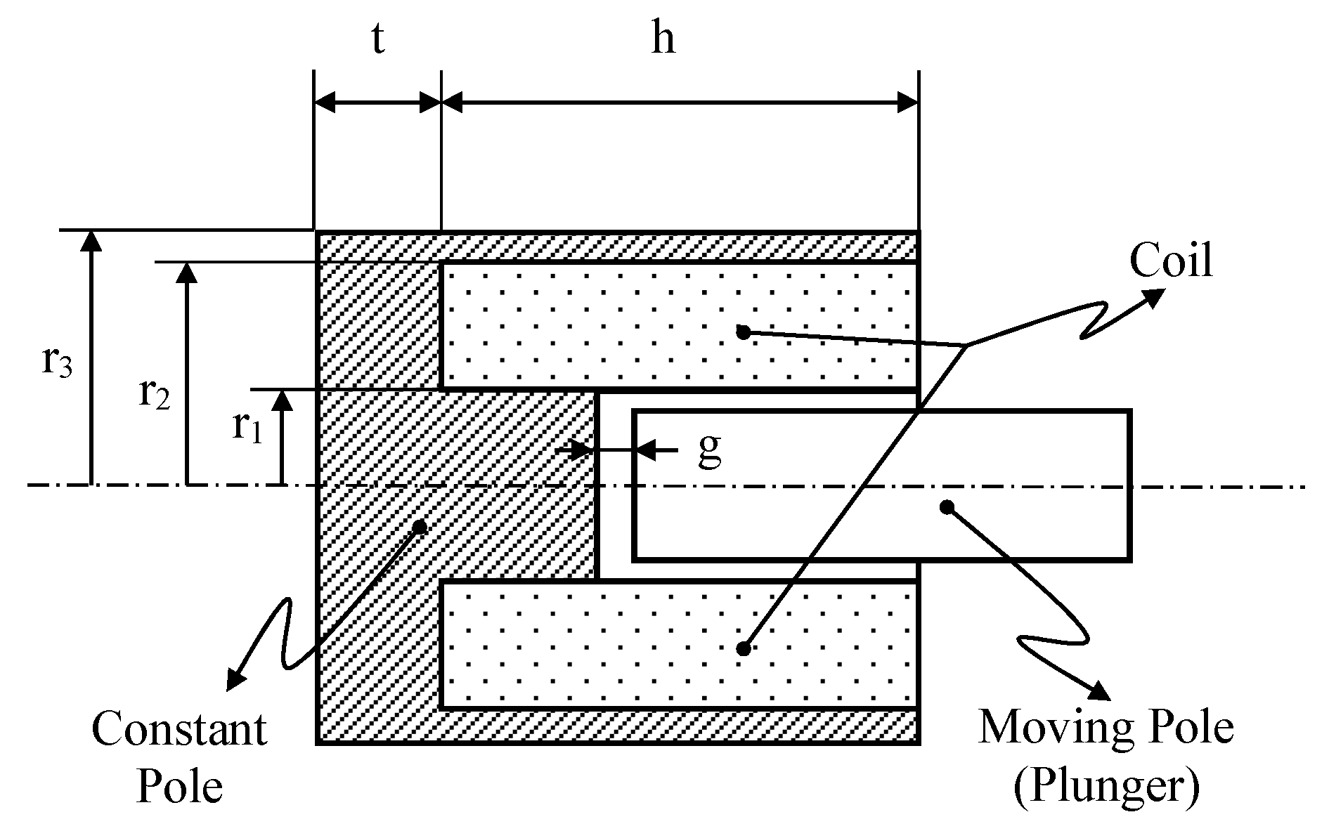
Figure 2.
A typical proportional solenoid characteristic
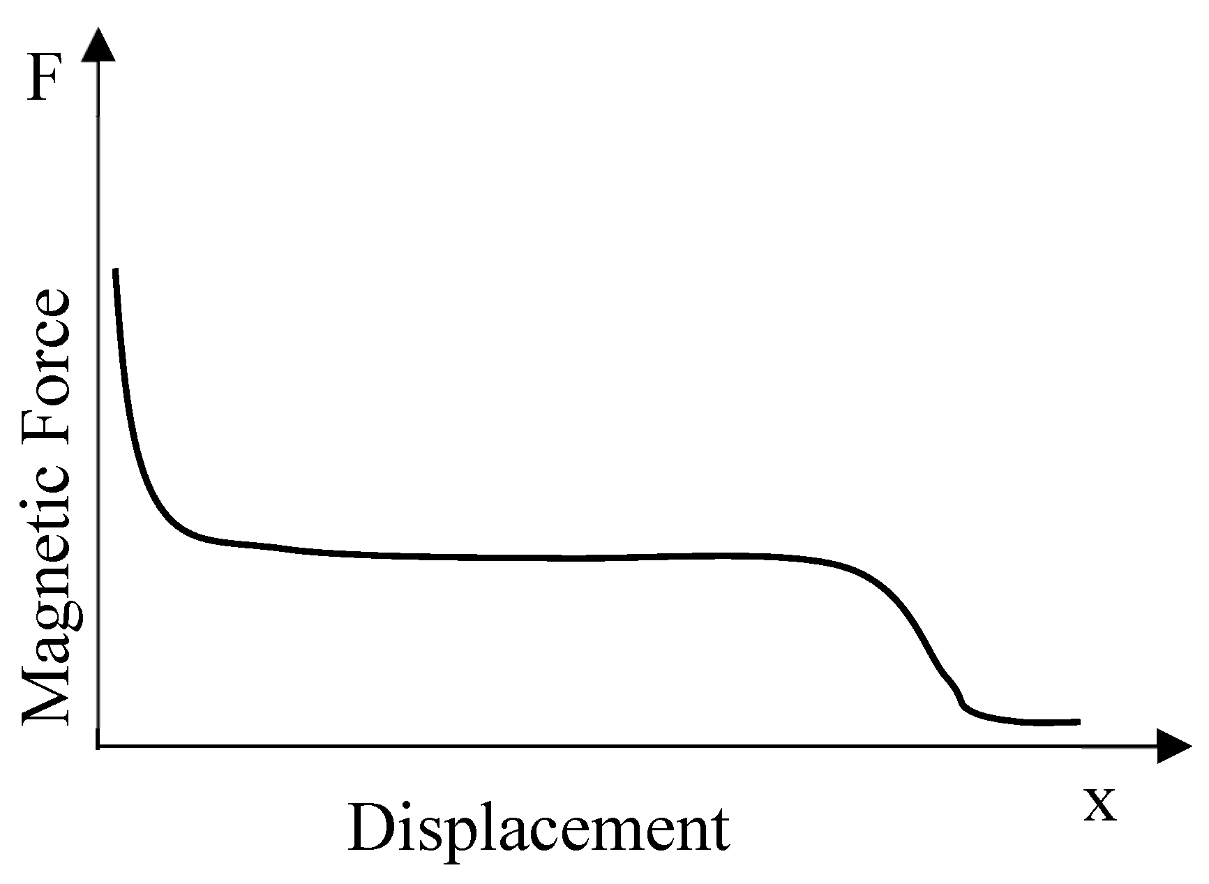
Figure 3.
Geometry parameters and definitions
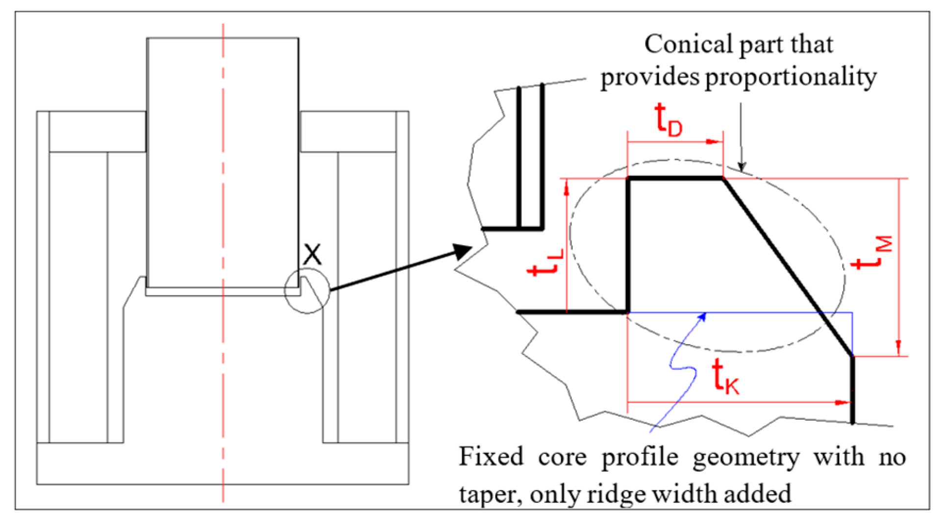
Figure 4.
Effect of parameter change on force characteristic. (a), (b), (c).
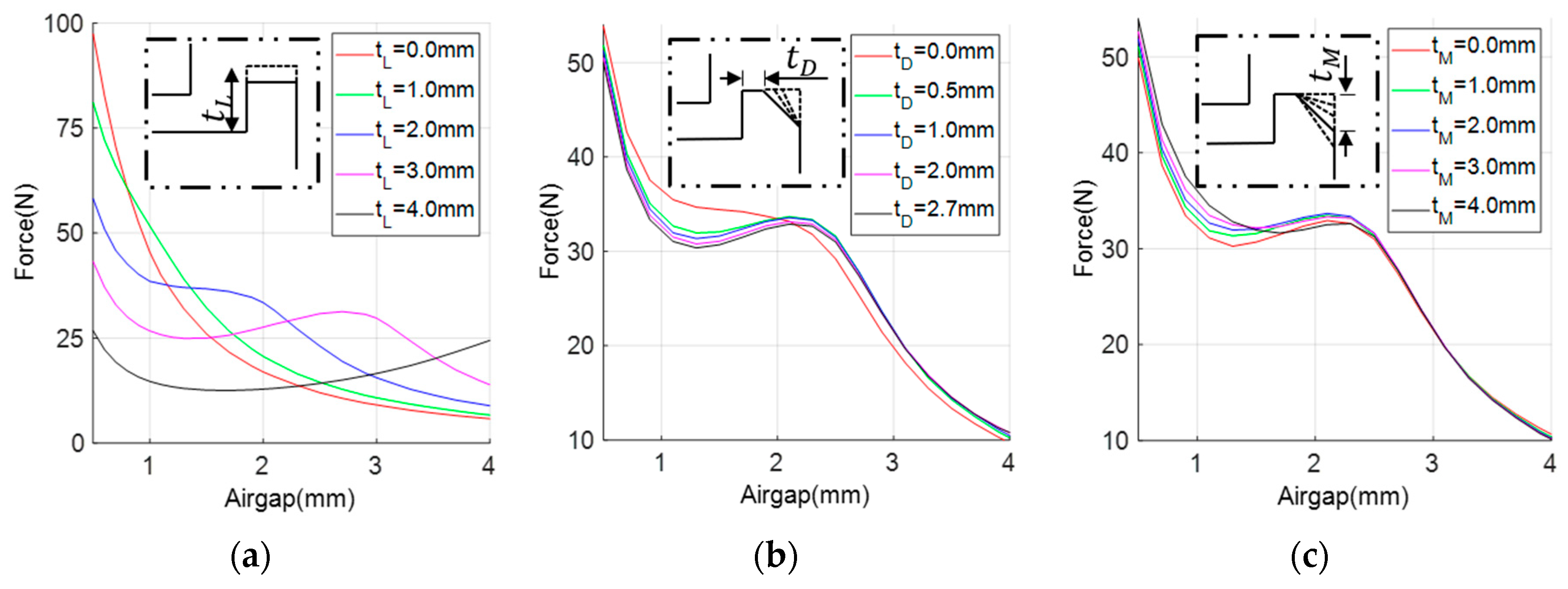
Figure 5.
Representative graph of the objective function
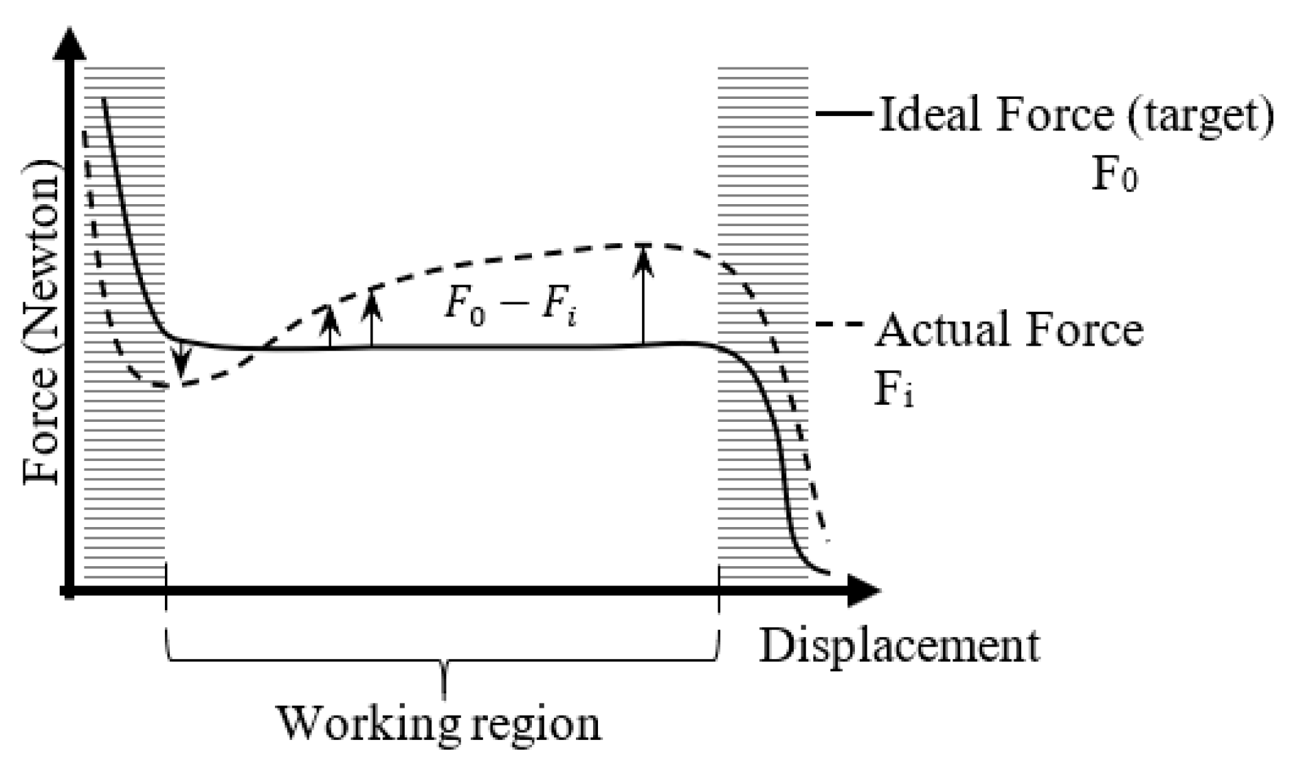
Figure 6.
Force characteristic for the parameters with the lowest objective function.
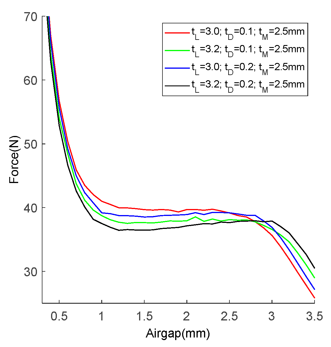
Figure 7.
The solenoid designed for g=0.1 mm: (a) Magnetic field strength (H); (b) Magnetic flux density (B) analysis.
Figure 7.
The solenoid designed for g=0.1 mm: (a) Magnetic field strength (H); (b) Magnetic flux density (B) analysis.
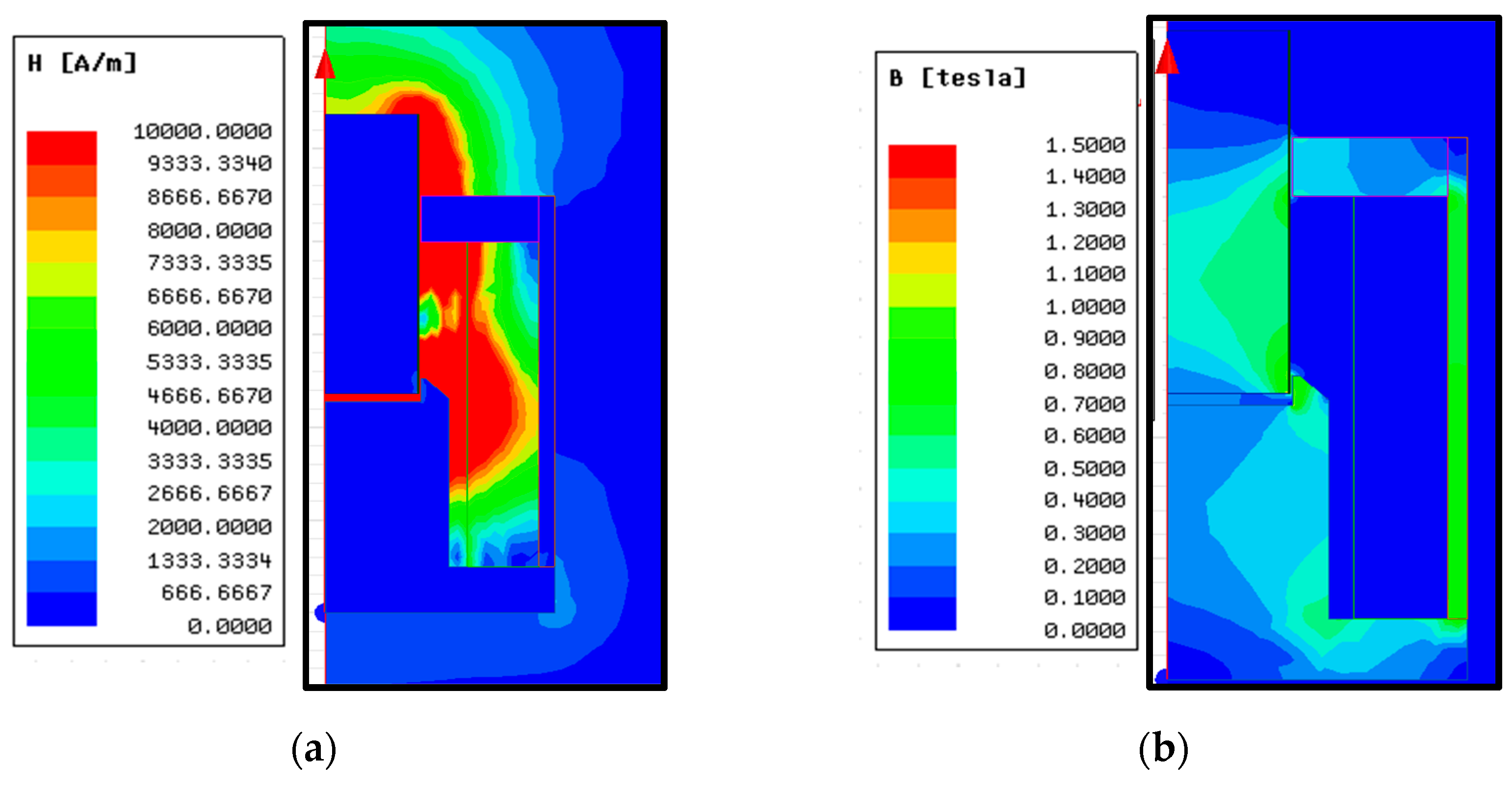
Figure 8.
Experimental setup for static characteristics
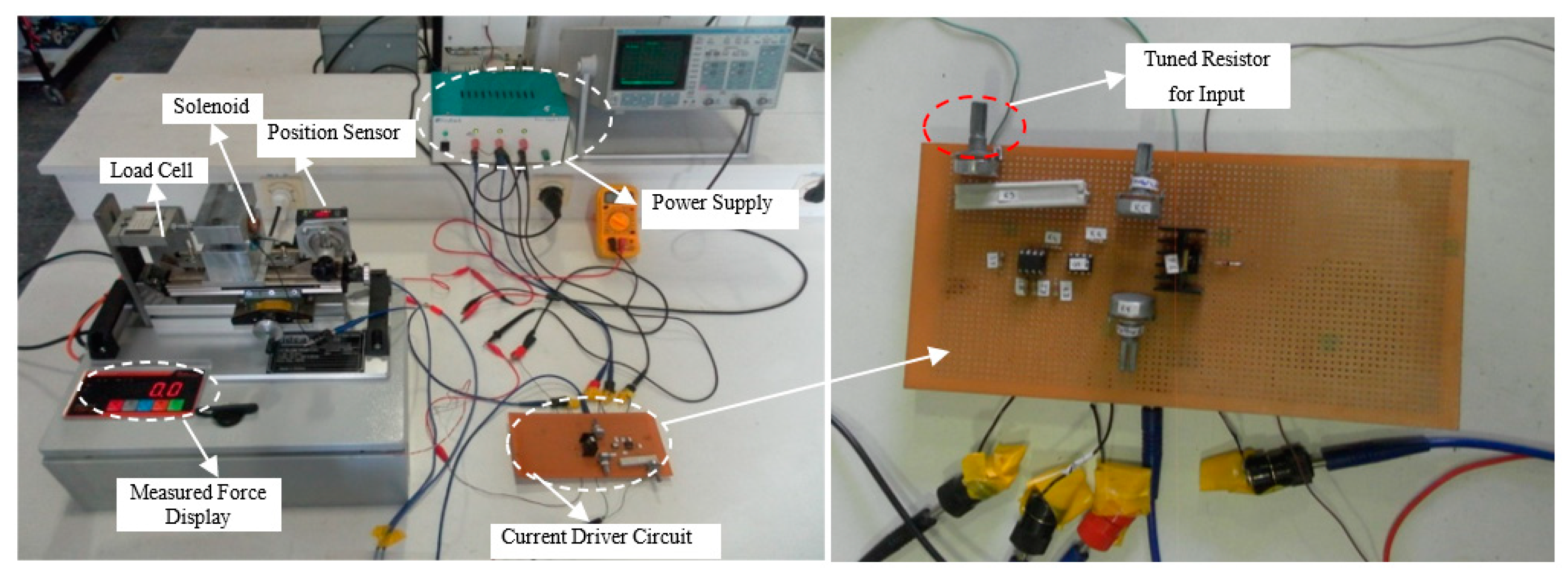
Figure 9.
Simulink model of the solenoid for dynamic behavior.
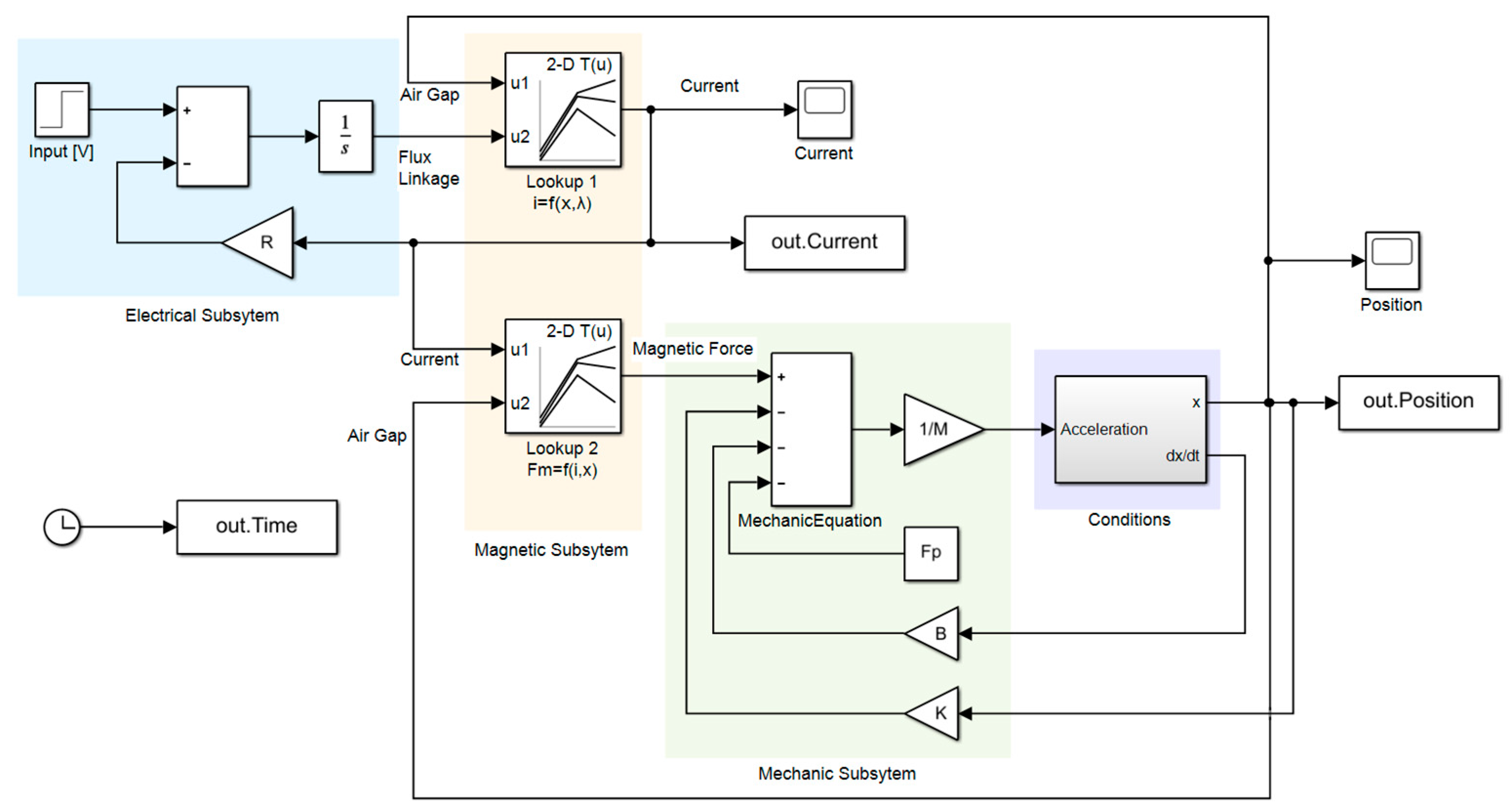
Figure 10.
Magnetic FEM analysis in the working region: (a)Airgap-Current-Magnetic Force; (b)Current-Airgap-Flux Linkage.
Figure 10.
Magnetic FEM analysis in the working region: (a)Airgap-Current-Magnetic Force; (b)Current-Airgap-Flux Linkage.
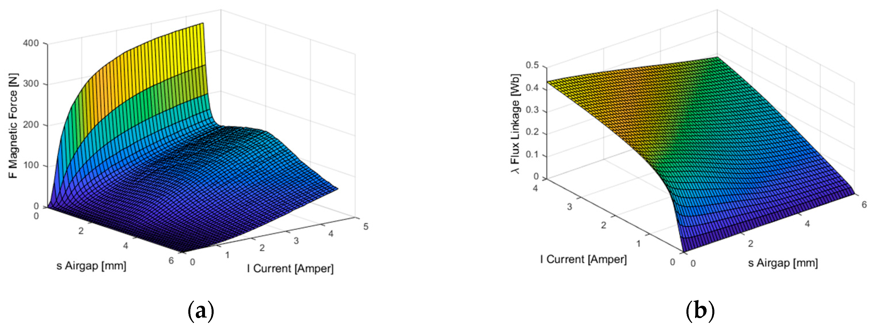
Figure 11.
Current and position characteristic obtained from the theoretical model.
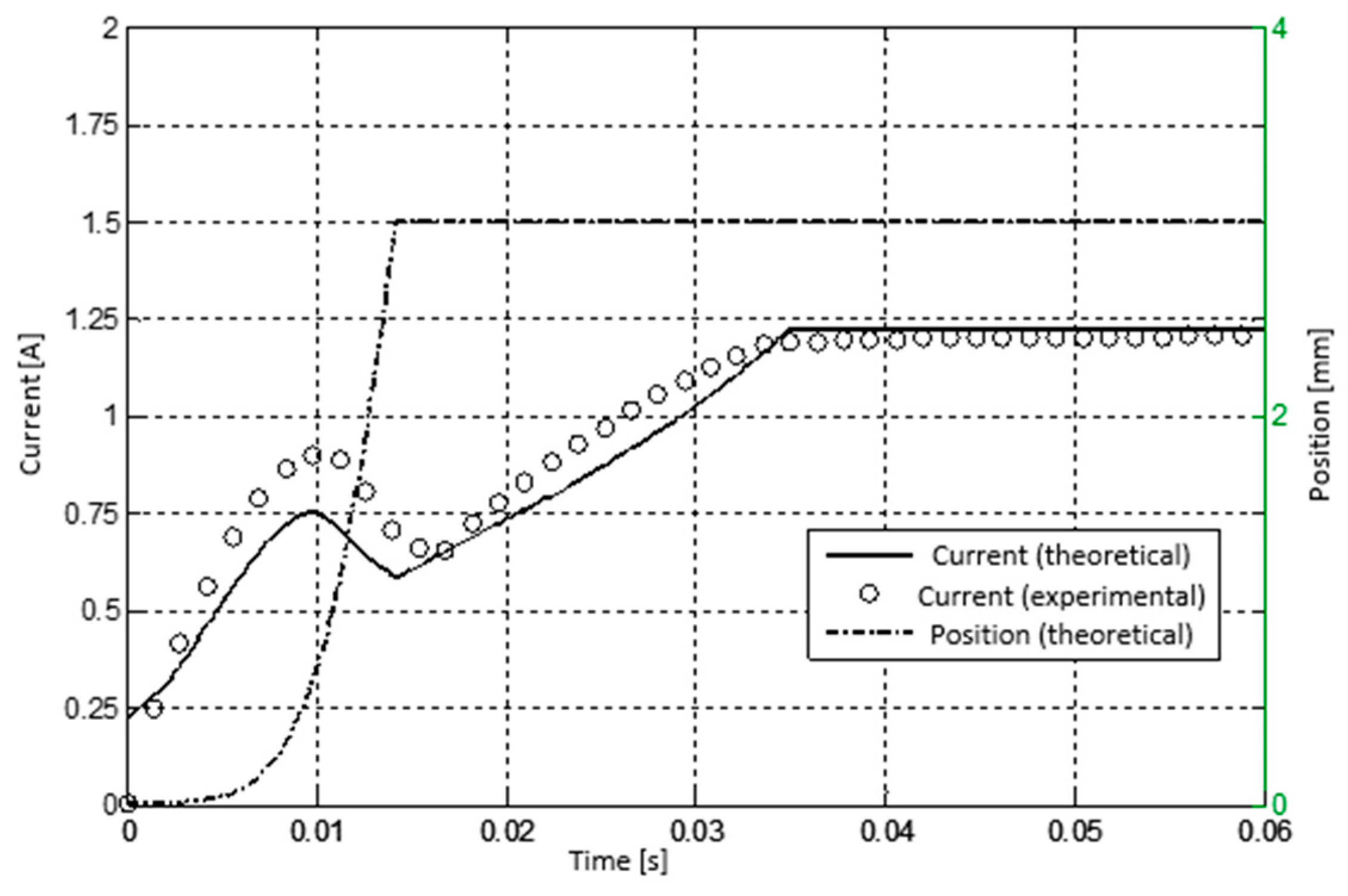
Figure 12.
Magnetic force (FEM Analysis): (a) Various current; (b) Various airgap.
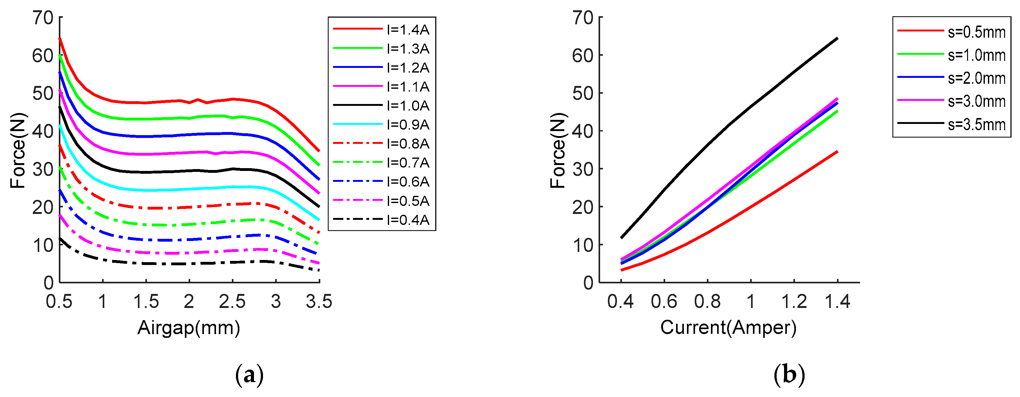

Table 1.
Dimensions of flat face piston-type electromagnet
| Symbol | Explain | Magnitude[mm] |
|---|---|---|
| Moving core radius | 9.00 | |
| Fixed part inner radius | 18.00 | |
| Fixed part outer radius | 19.50 | |
| Coil thickness | 9.00 | |
| Coil height | 35.00 | |
| Fixed part thickness | 7.00 |
Disclaimer/Publisher’s Note: The statements, opinions and data contained in all publications are solely those of the individual author(s) and contributor(s) and not of MDPI and/or the editor(s). MDPI and/or the editor(s) disclaim responsibility for any injury to people or property resulting from any ideas, methods, instructions or products referred to in the content. |
© 2024 by the authors. Licensee MDPI, Basel, Switzerland. This article is an open access article distributed under the terms and conditions of the Creative Commons Attribution (CC BY) license (https://creativecommons.org/licenses/by/4.0/).
Copyright: This open access article is published under a Creative Commons CC BY 4.0 license, which permit the free download, distribution, and reuse, provided that the author and preprint are cited in any reuse.


