Submitted:
22 October 2024
Posted:
22 October 2024
You are already at the latest version
Abstract
Global food insecurity and environmental degradation creates the need to develop more sustainable agricultural solutions. Plant synthetic biology emerges as a promising yet risky avenue to develop such solutions. While synthetic biology promises enhanced crop traits, it also harbors risks of extensive environmental damage. Here, we highlight the complexities and risks associated with plant synthetic biology, while presenting the potential of multilevel mathematical modeling to assess and mitigate those risks effectively. Despite its potential, the application of multiscale mathematical models in plants remains underutilized. We advocate for the integration of technological advancements in agricultural data analysis to foster a comprehensive understanding of crops across scales. By reviewing common modeling approaches and methodologies applicable to plants, the paper sets the stage for the creation and utilization of integrated multiscale mathematical models. Leveraging modeling techniques such as parameter estimation, bifurcation analysis, and sensitivity analysis, researchers can identify mutational targets and anticipate pleiotropic effects, enhancing the safety of genetically engineered species. To illustrate the potential of the combination, we outline ongoing efforts to develop an integrated multiscale mathematical model for maize (Zea mays L.), engineered through synthetic biology to enhance resilience against Striga and drought.
Keywords:
multiscale models
; synthetic biology
; systems biology
; mathematical models
; plant science
1. Introduction
The first green revolution successfully addressed the food crisis of the 1960s, by intensifying crop production under favorable environmental conditions with the aid of excessive fertilizers [1]. This approach led to an increase in the environmental impact of agriculture that will be charged to the current human generation [1]. These costs include land degradation with depleted soil’s nutrients, water eutrophication from fertilizer residues, over-extraction of groundwater, pest resistance caused by pesticide overuse, extinction of indigenous crop varieties, and increased greenhouse gases emissions that contribute to climate change [1,2,3]. Climate change triggers extreme weather conditions resulting in severe flooding and drought that jeopardize crop production in Asia [4]. Additionally, in sub-Saharan Africa, Striga hermonthica remains the most destructive pest, causing up to 100% yield loss in some crop fields [5]. In addition to the escalating climate crisis, ongoing conflicts, and recurring pest outbreaks are collectively undermining global crop production. For instance, the conflict between Russia and Ukraine is jeopardizing global maize production, as the two countries have a combined global production share of 17% for that cereal [6,7]. The continuous increase in world population also raises concerns about global food insecurity [8]. Projections by the Organization for Economic Co-operation and Development (OECD) and the Food and Agriculture Organization (FAO) of the United Nations (UN) estimate a world population of nearly 10 billion by 2050. This scenario is raising the stakes for sustainable food production and there are calls for a second Green Revolution that emphasizes production of crops that are resilient to suboptimal environmental conditions and create a more manageable environmental footprint [9].
To meet these challenges, researchers are turning to synthetic biology in plants, which employs biological engineering principles to improve beneficial plant traits in a way that goes beyond the speed and capacity of natural processes [10]. Through metabolic engineering and synthetic biology, plant scientists were able to remodel metabolic pathways to increase production of useful metabolites or inhibit synthesis of less useful ones [11]. Synthetic biology products that are now available in the market include Impossible Foods’ bleeding plant-based burgers, created from an engineered strain of the yeast Pichia pastoris that produces soy leghemoglobin and gives the burger a meaty sensation [12,13]. There is also Zymergen’s polyimide film, named hyaline, that is made from bio-sourced monomers [14], Pivot Bio’s biological nitrogen fertilizer for cereals [15], and Calyxt’s high-oleic oil from soybeans called Calyno [16,17]. More recently, printed vegan salmon also became available in supermarkets and many vegan fish alternatives are currently being developed [18]. As such, plant synthetic biology holds immense potential to steer agriculture towards a more sustainable future, alleviating global food insecurity.
While redesigning crops through plant synthetic biology is undeniably promising for the future of agriculture, it can also cause environmental damages. One of the risks that comes together with synthetic biology is producing a genetically engineered species that may increase ecosystemic problems once released into the natural environment [19,20]. Engineering plant genes may also initialize pleiotropic effects to the organism, due to off-target effects that can lead to unforeseen changes in the target species [19]. These risks can be mitigated using the combination of plant synthetic biology and mathematical modeling, which allows identification of mutational targets through the use of parameter estimation, bifurcation analysis, sensitivity analysis, and optimization [21,22].
To improve risk mitigation, integrated mathematical models should be applicable at different levels and with varying granularity. This is so because plants are complex systems composed of roughly modular components, and this modularity extends from the genome level to the tissue and organ levels [23]. However, the application of multiscale mathematical models, while frequent in microbial systems [24,25,26,27], remains underutilized in plants. Integrating technological advancement in the analysis of available agricultural data facilitates comprehensive understanding of crops, from genotype to phenotype to ecosystems, promoting effective environmental conservation and higher agricultural productivity [28,29].
To potentiate the creation and use of multilevel modeling in plants, this work reviews common modeling approaches and methodologies applicable to plants at various scales, from molecular to crop levels. We will focus on the most commonly used approaches, progressing from the simplest to the more mathematically complex methods. We also explore alternatives for integrating models across scales, discussing advantages and shortcomings of each approach. Our review concludes with insights into our ongoing efforts to create an integrated multiscale mathematical model for maize, modified through synthetic biology to be more resilient through enhanced resistance against Striga and droughts.
2. Model Building
Building multiscale mathematical models in plant synthetic biology remains a challenge, and as the model becomes more complex, so does its mathematical analysis. Further, integrating models of different levels and granularities poses additional complex challenges. In response to these challenges, we outline an iterative workflow for constructing a multiscale mathematical model in plant synthetic biology.
In Figure 1, we represent two nested cycles that summarize that workflow, portraying a minimalistic methodology for mathematical modeling that traverses across multiple scales from the molecular to the plant level. The flow in the inner cycle tackles the choice of methodology for model building and analysis, while the outer cycle portrays the integration between different scales of the plant processes one wants to model. The inner workflow applies individually at each step in the outer cycle to build a multiscale mathematical model of a plant. We should be able to use this model, once validated, to predict unintended pleiotropic effects of manipulating the genome on the plant at multiple levels.
In the remainder of this section we will review modelling strategies used in plants at various scales, from molecular to plant level. We will frame that review from the perspective of the workflow summarized in Figure 1. We note that the various stages proposed in Figure 1 may unfold to include more or less detailed modeling of the various plant subsystems. For example, shoot architecture may be modeled from a coarse level to a level where branching, leaves, and flowers are considered in detail.
2.1. Metabolic Modeling with FBA, Kinetic, or Hybrid Approaches
2.1.1. Applications
Metabolic modeling techniques, such as flux balance analysis (FBA), kinetic modeling, and hybrid approaches, play a crucial role in driving metabolic engineering towards efficiency [30]. Within the iterative design-build-test-learn (DBTL) cycle of metabolic engineering, metabolic modeling emerges as a valuable tool [11,31]. It offers a unique perspective on plant metabolism, yielding quantitative insights and informing new engineering strategies [31]. Particularly, it streamlines the trial-and-error cycles inherent in metabolic engineering, saving considerable time and resources [11,32,33].
We need to collect pathway data in order to build a metabolic model and mathematically represent it for analysis. When pathways are unavailable in databases, reconstruction and inference based on literature or genome analysis are necessary. This can involve utilizing gene sequences to identify related pathways and their data. Once we define the relevant pathways, we can associate a stoichiometric matrix to the system and use it for model construction. Additionally, preexisting kinetic information is often required for model creation and analysis. Table 1 provides a sample of databases containing kinetic and pathway data that are available to the reader for reference.
Most studies modeling plant metabolism employ Flux balance analysis (FBA)-based or kinetic-based models [31,33]. Flux balance analysis (FBA) stands out as a prevalent constraint-based approach for analyzing material and energy flow within metabolic networks [34]. Its advantage lies in the ability to analyze entire metabolic networks without detailed process mechanism information. FBA models have been extensively used to study plant metabolism, including in Arabidopsis thaliana, tomato, maize, and rice [35,36,37,38,39,40,41,42,43,44,45,46]. They facilitate understanding flux distributions and gene essentiality, requiring modest prior information.
However, FBA has limitations. It cannot accurately represent regulation and lacks information on transient responses or metabolite concentrations, crucial in metabolic engineering. For such cases, more detailed kinetic models are necessary, either developed from scratch or based on simplified FBA versions. Kinetic models offer mechanistic descriptions of metabolism, enabling regulation incorporation but demanding more prior information. They require knowledge of individual metabolic processes and parameter values for rate expressions, often obtained from databases like BRENDA, MetaCyc, or KEGG (Table 1). When using these databases, it is important to be aware that parameter values are frequently determined in vitro, and might be significantly different from in vivo values [33].
As FBA models, kinetic models can be used to analyze steady state flux distributions. In addition, they provide information about transient flux changes and concentrations, both at steady state and during transient responses. This is required in situations where metabolic engineers need to predict behavior of the biological system under genetic or environmental perturbations [33]. In addition, kinetic modelling enables sensitivity and stability analysis, which provide a framework for elucidating parameters responsible for the control of metabolic fluxes in a network [33,47,48,49].
Kinetic models typically focus on smaller parts of the metabolic network [31], employing rational expressions like Michaelis-Menten or Hill equations [50,51,52,53,54,55,56,57]. Other typical kinetic expressions include mass-action and Arrhenius equations [58], saturable and cooperative formalisms [49,59,60] as well as generalized mass action (GMA) kinetics [48,61]. GMA and other approximate representations are very useful when the mechanism for the individual processes is unknown [59,60]. Kinetic models were used to study, among other things, the flavonoid biosynthesis pathway in Arabidopsis thaliana [58] and tomato [54], central carbon metabolism in potato [55], central carbohydrate metabolism [53], aspartate-derived amino-acid pathways [51], and 2-C-methyl-D-erythritol 4-phosphate (MEP) pathway [56] in Arabidopsis thaliana, benzenoid network in Petunia hybrida [52], lignin biosynthesis in Brachypodium distachyon [61], and nitrate reductase activity [50].
FBA and kinetic models can sometimes be combined into hybrid models [33]. By integrating both methodologies, hybrid models overcome limitations and enhance model power. Creating a hybrid model is a two-step process that involves creating an FBA model to generate flux distributions, then using these distributions to estimate parameter values for kinetic sub-models. Hybrid models provide detailed concentration insights from kinetic modeling while validating results with FBA outputs, offering a more accurate representation of real-world metabolic processes [62]. Another parameter determination approach is ensemble modeling which calculates the parameter values with references to the steady state fluxes [31,63].
2.1.2. Creating a Metabolic Model
Figure 2 summarizes a typical workflow for metabolic modeling with FBA, kinetic, or hybrid approaches. Here, we illustrated the input, method/approach, and output of a plant metabolic model. Let us now look at the modeling process in more detail. In general, given that we a have a metabolic pathway with number of metabolites and n number of reactions/fluxes , we can generate an by stoichiometric matrix [64,65,66,67]. After obtaining the stoichiometric matrix , we can build a flux vector with by 1 dimension where each row is the flux . Then, we apply matrix multiplication to and to get the metabolite/substrate vector with by 1 dimension where each row represents the rate of changes of each . We represent this mathematically using Equation (1).
From equation (1), we diverge into different paths depending on the modeling approach. To create an FBA model, we assume a steady state of flux where the rate of changes in vector M is zero, that is . Hence, Equation (1) becomes
At this stage we constraint the flux vector v using an objective function that could, for example depend upon the rate of material/energy entering and leaving the system and the minimal and maximal amounts of that flux that need to flow through different sub-processes for the system to be viable. We can then use linear optimization to solve the flux distribution and find the appropriate solutions to that optimization problem.
In constructing a kinetic model, we begin with Equation (1) and select suitable mathematical formalisms to represent the kinetics of individual processes and their dependence on substances directly influencing flux. Various formalisms, including linear, rational, and power laws, among others, are available [60]. Each formalism is associated with parameters whose values need to be estimated to predict the dynamic behavior of the model quantitatively. We can obtain initial parameter estimates for example from databases listed in Table 1 or from primary literature sources.
Equation (1) is equivalent to which is a nonlinear ODE. In analyzing nonlinear ODEs, a common practice is to approximate using linearization of the system. To linearize Equation (1), we calculate the Jacobian matrix (J) by getting the partial derivative of each ODE with respect to each dependent variable.
Using the Jacobian matrix (J), we determine the stability of the system through the computation of the eigenvalues of the matrix J. The real part of the eigenvalue of a stable system must be negative for the steady state to be stable. With this into consideration, we use different methods to understand how certain factors affect the concentrations of metabolites. For example, sensitivity analysis [65,66] helps us identify which parameters can cause significant changes, parameter scanning helps us gauge the extent of these changes, and time-series analysis helps us track how metabolite concentrations change over time [48,57].
From Equation (2), the output of FBA yields a flux distribution v that minimizes or maximizes the given objective function. Common applications of these models involve modifying constraints and initial conditions or altering the system by removing selected processes from the diagram, thus assessing their impact on the model's solution space. On the other hand, the output of the kinetic model encompasses all metabolic concentrations involved in the metabolic pathway, offering a comprehensive view of the system's behavior under specified conditions.
2.2. Shoot and Root System Architecture
Shoot and root plant system architectures are essential for resource acquisition during plant development. Yet, conducting plant experiments, especially in the field of plant synthetic biology, is inherently challenging with respect to time and cost. It is also hard to estimate the risk of disrupting local ecologies when introducing new plant varieties. Developing a 3D architecture visualization model is crucial to predict plant shoot/root growth and development, facilitating reasonable approximate estimations of crop productivity [68,69]. Thus, there has been a growing interest in building mathematical models of the shoot and root system architecture to do in silico investigation in plants. However, this field is still less mature than that of metabolic modeling and methodological development is ongoing.
2.2.1. Shoot System Architecture
2.2.1.1. Applications
The shoot system architecture (SSA) is generally the above ground portion of the plant that consists of stem, leaves, buds, flowers, and fruits. Optimizing the shoot growth of wheat revolutionized agriculture during the 1960s resulting in the First Green Revolution. First, the agronomist Norman Borlaug developed a high yield and disease resistant wheat variety [70,71]. However, the wheat stalk of this variety was too thin to support the weight of its own grain, leading to a type of breaking called lodging. Thus, he further developed a dwarf variety of this wheat which can bear heavier weight [71]. This development of dwarf wheat solved an impending global food crisis during that time.
Creating dwarf wheat through traditional breeding took many years [72]. With the current gene editing technology, it is already possible to speed up the process of developing more desirable plant varieties, creating specific modifications in the genome of plants to obtain specific traits. Using models to simulate the effects of these genetic modifications on the phenotype of SSA could mitigate risk and predict the quantitative effect of genetic interventions on shoot traits and crop yield more accurately. This could speed up the process of producing new crop varieties.
There are several models for SSA that have been developed over the years [73,74,75,76]. L-systems underlie many of these models [73,76,77,78,79,80,81,82,83,84,85,86,87]. This modeling formalism was named after Aristid Lindenmayer, and it is widely used to model plant morphogenesis [88]. In Table 2, we listed several functional-structural plant modeling (FSPM) platforms from the Quantitative plant website [89]. We can also use these platforms to model root and whole plant architectures.
2.2.1.2. Creating a Shoot System Architecture
In Figure 3, we present a workflow for building a SSA model. Initially, we need to determine whether the plant species is monocot or dicot, as they have different architecture from one another. A monocot generally has tillers, with secondary shoots branching from its primary shoot. A dicot typically has only one primary shoot [90].
In modeling SSA, we need to describe the phytomers, which are the fundamental structural units of the shoot. These phytomers are produced from shoot apical meristems (SAM), also called terminal bud [74,76,91]. Figure 3 shows an example of phytomers. There, each phytomer is a stem segment that is composed of a leaf, an axillary bud, a terminal bud, a node, and an internode. The phytomers are stacked up to form a shoot, whose form may vary depending on the plant species. Wen et al. [76] defined a geometrical model of a shoot as
Here, and describes the rotation and translation of the and the is the union of number of phytomers.
We can use these models to quantify shoot architecture traits such as leaf area (an important factor for capturing light), plant height, stem length, volume, etc.
2.2.2. Root System Architecture
2.2.2.1. Applications
The most frequently used root phenotyping techniques include shovelomics, the monolith method, and X-ray computer tomography [92,93,94]. Shovelomics [92] is a rapid and high throughput phenotyping method. This is done by digging a shovel size portion of the root and then manually measuring 10 root architectural traits. The monolith method [93] uses a steel cylinder with 20 cm diameter and 30 cm depth for excavating roots and measuring their phenotypes. This method allows excavation of deeper roots and uses a root image analysis software to quantify root traits. More recently, X-ray computer tomography (CT) was used for 3D visualization that captures more detailed root architecture traits [94].
In comparison to shoot, root data gathering is particularly challenging. This difficulty exponentially increases as the roots continuously grow deeper into the ground. Thus, the development of easy-to-use methodologies to facilitate root phenotyping is still an important unmet need. The belowground disposition of the root makes it more beneficial to simulate a 3D visualization of the root system architecture (RSA), when compared to SSA. Similarly to SSA, the most common approach in modeling RSA is also the L-system [88,95].
Researchers have long been engaged in constructing virtual models of roots and on using those models to simulate the effect that changing environmental conditions has on the RSA, with the aim of prioritizing interventions that might increase crop yield [96]. The development of root modeling platforms dates back to the 1970s [97,98]. Later, more advanced modelling platforms were created. ROOTMAP [99] is a notable 3D model focusing on fibrous root systems and their proliferation. Other platforms, like RootTyp [100,101] and DigR [102], highlight the influence of soil in root development, while SPACSYS [103] delves into root-soil interactions and their impact on crop yield.
Unlike metabolic models or SSA models, many RSA modeling platforms are not publicly available [104]. This hinders the advancement of the field. The rise of open science spurred initiatives like OpenSimRoot [105] , an open-source 3D RSA model accommodating various plant species and focusing on nutrient acquisition's feedback to root development. Similarly, CRootBox [106], derived from RootBox [95], fills the gap between in situ and in silico studies by integrating 3D RSA simulations into experimental setups such as cylindrical pots and rhizotrons.
These platforms contribute to untangling the complexities of RSA. More recently, a modeling study [107] proposed an approach for predicting root/shoot system architectures. Their iterative and stochastic method generates elongation length, root direction, and branching until building an individual plant root architecture. Notably, their approach allows for modular introduction of hormonal and metabolic factors influencing architecture development, predicting their effects on various root traits like length, branching, volume, and surface area.
2.2.2.2. Creating a Root System Architecture
Figure 3 summarizes a three-step workflow for building models for root system architectures (RSA). In a parallel situation to that of plant shoots, plant roots may be classified either as tap root for dicots or fibrous roots for monocots. Taproots have one primary root (or main root axis) while fibrous roots have several additional root axes, for example seminal and nodal roots. As such, the initial step in creating a model for a RSA is to decide which type of root one needs to model.
Subsequently, we need to define a root axis for the RSA model. Figure 3 illustrates a root segment of the RSA, consisting of a main root axis that displays secondary root branching in the form of lateral roots. This main root axis accurately represents a taproot. For modeling fibrous roots, we need to generate additional axes that describe seminal and nodal roots.
A step-by-step description of such a model building process can be found in a recent literature [107]. That process requires defining at least two parameters: the growth elongation rate and the growth angle, which are important for growth elongation rate and growth angle, respectively. We initialize the root system architecture is initialized at the origin in 3D space. Iteratively, the approach decides the magnitude of the elongation and direction of the root for each step. Stochastically, we define branching points from where secondary roots will branch and grow, generating a full architecture. This model outputs a 3D visualization of the RSA of a plant, something hard to image experimentally. After generating the RSA, we can also quantify length, branching, volume, surface area, and other traits of the RSA.
2.3. Resource Acquisition
Resource acquisition in plants encompasses obtaining energy and fixing carbon via photosynthesis and collecting mineral and fixing nitrogen through the roots. Modelling plant resource acquisition is often but not always connected to modelling RSA and SSA. Understanding how changes in SSA or RSA influence light acquisition via photosynthesis and water and mineral nutrient uptake from the soil is usually the primary objective of resource acquisition models.
In the context of resource acquisition, researchers use 3D SSA/RSA models to identify factors that change the architectures in ways that maximize a plant’s resource acquisition. Examples include modelling the effect of changing leaf’s area on the amount of light captured by the plant [108,109,110], or simulating the effect that changing spread and depth of root into the soil has on mineral, nitrogen, or water uptake through the root [111].
2.3.1. Photosynthesis
2.3.1.1. Applications
Photosynthesis sustains life on our planet through the supply of food and oxygen [112], allowing plants to grow, develop and reproduce [113]. This process lets plants capture energy from light, use that energy to fix atmospheric carbon from CO2 into sugar, and release oxygen into the air as a byproduct.
Photosynthesis has two phases. The first phase converts energy from light into a chemically usable form. The second phase fixes atmospheric CO2. By and large there are three different types of metabolism to fix that CO2: -, -, or Crassulacean acid metabolism (CAM) [113,114,115].
Figure 4 illustrates how to model photosynthesis. The process initiates with the decision regarding which type of metabolism needs to be modeled (–, –, or CAM). Model inputs always include (but are not limited to) light and . Regardless of the type of photosynthetic metabolism, three broad approaches can be used to build the model: empirical, mechanistic, or hybrid approaches that combine the first two [113]. In addition, and independent of the approach, the models can be either deterministic or stochastic and simulations can run on continuous or discrete time steps. This study [113] highlighted that decisions regarding which approaches to use should consider minimizing the number of model parameters and correctly representing physical, chemical, and biological laws. One should also consider minimizing the variance of the simulation outputs and the deviation between predicted model values and measured experimental values.
2.3.1.2. Creating a Photosynthesis Model
The Farquhar – von Caemmerer – Berry (FvCB) model pioneers mathematical modeling of photosynthesis of plants [114]. The FvCB model calculates the assimilation using Eq 4 [113,114,116]:
Here, and represent carboxylation rate and oxygenation rate, respectively, and is the mitochondrial respiration rate.
C4 photosynthesis relies on the coordination between mesophyll and bundle sheath cells within leaves. Initially, CO2 is fixed into a C4 acid, likely in the mesophyll, by phosphoenolpyruvate carboxylase (PEPC) [115,117]. This 4-carbon compound then moves to the bundle sheath, where it undergoes decarboxylation, providing CO2 for Rubisco to initiate the regular C3 carbon fixation process. Therefore, modeling C4 photosynthesis entails additional initial steps, along with a mathematical model of C3 photosynthesis (see [115] for details).
Plants in arid regions, characterized by less than 25 cm of rainfall per year, have adapted to dry environments by evolving CAM metabolism, a type of photosynthesis that fixes CO2 more efficiently while reducing evapotranspiration. CAM photosynthesis operates through a circadian metabolic cycle, with stomata opening at night and closing during the day to minimize water loss. During the night, PEPC fixes CO2 to produce malic acid, which is stored in the cell vacuole. During the day, the vacuole releases malic acid, which is then decarboxylated through the Calvin Cycle. Recent review [118] presented several mathematical models of CAM photosynthesis, including ODE-based models [119,120,121] and FBA – based models [122].
In photosynthesis models, the typical output variable is the rate at which plants fix atmospheric CO2 and/or the rate at which plants use that CO2 to produce sugars and other compounds. Various definitions of photosynthetic rate exist in the literature, all linked to the plant's use of atmospheric CO2 to produce sugars [113,114].
2.3.2. Nutrient Uptake Model
2.3.2.1. Applications
One of the primary functions of roots is to acquire water and nutrients from the ground and supply them to meet the metabolic needs of plants. Nutrient acquisition models are normally layered on top of RSA in silico models [105,106,123,124]. These models are very useful to investigate the effect of rapidly changing environmental conditions on plant growth, and prioritize which costly field trials to make [125], saving time and money. They are also useful in combination with traditional approaches to develop innovative practices in fertilizer management [126]. In addition, quantifying root nutrient uptake provides insights into potential crop yield.
Over the years, the development and application of several models to quantify root nutrient uptake has been on the rise, aiming to optimize fertilizer usage in agriculture. Initially, nutrient uptake was modeled as directly proportional to the available nutrient concentration in the soil, with root absorption power serving as the constant parameter [127]. However, solving the system of partial differential equations (PDEs), whether analytically or numerically, posed a significant challenge. To address this issue, a study [128] introduced the Crank-Nicolson method to numerically solve their nutrient uptake model. Building upon this approach, another study [129,130] incorporated root system growth into their models using the same numerical method. Later, the roots of rapeseed were modeled to investigate the influence of root hairs on the uptake of phosphorus [131]. These studies were extended [132] to other plant species, who quantified how plant phosphorus uptake strongly influenced the number, length, and radius of root hairs.
The Nye-Tinker-Barber (NTB) model became the most frequently used for modeling plant nutrient uptake [133,134]. A study [135] extended this model, demonstrating the existence of an explicit closed-form solution to the diffusion-adsorption problem [136,137]. Additionally, it was further extended [138] and analytical solutions were provided to convection-diffusion equations applicable to general solute nutrient uptake scenarios.
Recent advancements include the use of perturbation expansion methods to approximate nutrient flux and concentration solutions [139]. This approach divided the rhizosphere into inner and outer fields, aligning with the root surface, and derived approximate analytical solutions for nutrient uptake flux at the root surface and global nutrient diffusion of the NTB model. Another study [140] contributed to finding analytical solutions using Laplace transforms.
2.3.2.2. Creating a Root Nutrient Uptake Model
Figure 4 illustrates the modeling process of nutrient uptake, beginning with the definition of the biological problem. This involves identifying the specific nutrient being modeled, which can be categorized as either mobile (such as nitrogen, sulfur, boron, manganese, and chlorine) or immobile (including phosphorus, potassium, magnesium, calcium, copper, iron, and zinc) in soil. A classification of the mobility of mineral nutrients in soil [141] is presented in Table 3.
Following the classification of nutrients, diffusion equations mathematically represent the transport process from the soil to the root. These equations are typically described using PDEs, which incorporate both time and space as independent variables [142]:
where the concentration (c) changes over time (t) and the flux (J) depends on the spatial variable (x).
This simple diffusion equation becomes more complex as additional spatial features of solute transport are incorporated. A review study [143] categorized various solute uptake models from the literature based on their complexity, including those representing diffusion only, diffusion with advection, diffusion with reaction, and diffusion with both advection and reaction.
Once we have mathematically represented root nutrient uptake using PDEs, the next step is to determine their solution, which can be either analytical or numerical. While finding analytical solutions can be challenging, a widely used method is non-dimensionalization, which simplifies PDEs by introducing non-dimensional variables [135]. Non-dimensionalization facilitates the process of finding an analytic solution [144]. When analytical solutions are hard to find, we use simulations to find numerical solutions, often by discretizing time and space. A study [145] extensively reviewed different numerical methods for discretization.
After determining the solution, various analyses can be performed, including parameter estimation, sensitivity analysis, or prediction of soil nutrient uptake fluxes and concentrations.
2.4. Shoot-Root Interaction
2.4.1. Applications
The allocation of resources in plants is a crucial ability that determines their survival in challenging environmental conditions. Current climate trends emphasize the need for crops that have phenotypic plasticity and can adapt to growing with less water and more heat. This phenotypic plasticity comes from the capacity of a given genotype to express different phenotypes in response to varying environmental conditions [146]. Modeling shoot-root interactions is especially useful for simulating different scenarios and predicting the range of phenotypic plasticity of plants in different surroundings. In addition, modeling shoot-root dynamics allows for further exploration of plant productivity, considering the allocation of nutrient minerals from uptake and carbon from photosynthesis. This integration creates a multiscale mathematical model capable of facilitating in silico experiments ranging from the metabolic level to the whole plant level.
Researchers proposed many transport-resistance (TR) models to analyze plant growth dynamics. A TR model that pioneered this field [147] introduced a leaf-stem-root model that accounted for the utilization and transportation of photosynthate among different parts of the plant. In a subsequent study [148], they constructed a shoot-root model focusing on the exchange of photosynthetic output between the shoot (carbon) and root (nitrogen) uptake. Additionally, he incorporated the chemical and biochemical conversion of these substrates into structural dry matter [149]. This was expanded [150] by considering the effect of water potential and transpiration in his model. He utilized the Münch flow mechanism of phloem translocation and introduced a switch based on concentration gradients. In a more recent study focused on phosphorus dynamics [151], researchers combined experiments and models to investigate shoot-root interaction over a day-and-night cycle, using Petunia hybrida as a model organism.
2.4.2. Creating a Shoot-Interaction Model
Figure 5 outlines the modeling process for shoot-root interactions, depicting the input compartment consisting of resources acquired from photosynthesis and nutrient minerals from root uptake. These models primarily focus on resource allocation, emphasizing the exchange and transfer of resources between the shoot and root. In describing the utilization and transportation of substrate, most models employ the TR approach. This modeling approach is favored for its realistic representation of transport, accounting for substrate losses during transport and translating C/N fixation into root growth, using functions that convert volume into plant structure [154].
Still, different models use alternative strategies. For example, the teleonomic model [148] prioritizes factors like the shoot-root ratio, growth, and substrate concentrations based on environmental conditions [155]. Other models give more importance to other factors, such as soil water potential and root temperature effects on plant partitioning of photosynthate [156].
Regardless of the approach used, shoot-root models need to account for the interactions between two interconnected compartments: the shoot system and the root system [151]. The shoot part may range from simple shoot concentrations of substrates to more complex models specifying shoot concentrations of stored starch and soluble sugars, including shoot structure/architecture and mineral nutrients from the roots such as nitrogen, phosphorus, and potassium [124,152,157]. Similarly, the root part comprises exchanged substrate concentrations from the shoot, root structure/architecture, and nutrient uptake from the soil [151,152]. The exchange of soluble sugars from the shoot and mineral nutrients from the root is driven by a transport function [149], with the growth rate dependent on the substrate concentrations it contains.
These models often output the concentration of different substrates for shoot and root over time, mathematically represented by ordinary differential equations (ODEs). Thus, they enable in silico stability and sensitivity analysis of the shoot-root ratio under various environmental conditions.
3. Discussion
3.1. The Potential of Multiscale Mathematical Modeling
Plant synthetic biology aims to engineer plant biological systems to improve crops through direct manipulation of genetic circuits in plant genomes [10]. Given the complexities of such manipulations, they come associated with potentially serious biosafety risks [19,158]. Multiscale mathematical models can be a valuable tool for risk mitigation through the in silico simulation and analysis of those effects. These models provide another layer of quality control for the design stage of design-build-test-learning (DBTL) cycle of synthetic biology [159]. Ultimately, this approach can expedite the development of new crop varieties and reduce the costs associated to that development [160].
While crucial to test the effect of interventions, traditional plant breeding techniques and experimental studies are time-consuming and unpredictable [71]. We can use multiscale mathematical models to predict the effects of genotype modifications on the plant’s phenotypic traits. Integrating in silico investigation through multiscale mathematical models into the DBTL cycle of synthetic biology enhances speed and accuracy of predictions made about for the effect of genome manipulation on in planta implementation [160,161]. In addition, we can fine-tune their precision in quantifying the changes caused by the genetic intervention to molecular, architecture, resources, and whole-plant levels by incorporating experimental information that becomes available during the model building process.
Understanding and correctly representing the interplay between those levels is crucial for improving plant growth and productivity and optimizing fertilizer management while reducing environmental impacts. For instance, growing shoots and roots are responsible for resource acquisition, which is then used to produce sugar that is consumed for the shoot and the root to continue to grow. Several studies [162,163,164] pinpoint the influence of carbon, nitrate, and sugar in shoot and root development. This and many other nonlinear internal feedback loops naturally exist in biological systems [57,165]. Accurately predicting the effect of those regulatory loops on the dynamic behavior of the plant requires using multiscale mathematical models. The predictions can subsequently be validated in comparison to experimental evidence [28]. There is a review [166] of several designs of synthetic gene circuits for plants which can be modeled using a multiscale mathematical model [28] and following the methodology that we presented in Figure 1.
Account for the complexity of plant systems requires multiscale mathematical models, as single-scale models cannot capture the intricate dynamics of the whole system [167]. Figure 1 illustrates an iterative process for creating these models, allowing entry at any step of the model building process. This approach helps understand how molecular changes propagate throughout the organism, informing strategies for genome modification to achieve specific objectives.
Despite the beneficial contribution of this approach to the advancement of plant synthetic biology, there is a significant gap between scales when it comes to available knowledge and methodological tools for creating and analyzing models at each scale. This is evident when comparing for example metabolic level models to shoot/root system models. Such gaps complicate the integration between scales within a model. This integration is crucial for evaluating how genetic manipulations interact with environmental and metabolic cues, influencing plant development. The modular nature of plant systems suggests an approach to facilitate scale integration in multilevel models: make the models representing the different levels as modules [27,28,168]. Also, there is a continuous effort to build Crops In Silico [167], which is a platform for plant mathematical models highlighting the value of multiscale approach.
A critical aspect in doing so is describing the connections between scales or translating the output of a model from one scale as input into another. One solution is to represent each scale in a separate submodel, using appropriate mathematical representations and tools, and interconnect them through relevant variables. This approach has been successfully applied to create multiscale mathematical models of several microorganisms [24,25,26,27].
The development of useful multiscale plant models depends on accurate parameter measurements. Advanced plant phenotyping technologies [92,93,94] are leading to an era of big data, providing modelers with highly accurate measurements. A study [169] proposed a modeling workflow centered on digital twins, using X-ray computed tomography (CT) to capture detailed root images for constructing root skeletons and RSA models. This approach allows for comprehensive analysis of plant phenotyping data, providing deeper insights into various plant functions [170]. While another study [107], modeled of the effects of varying concentrations of strigolactones on RSA demonstrated changes in root elongation and lateral root branching density.
The construction of whole-plant digital twins is likely to be forthcoming. Building whole-plant digital twins will likely be facilitated by artificial intelligence (AI). AI algorithms can analyze experimental data to inform model-building choices and later analyze data generated from digital twins, offering insights into plant growth, development, and responses to environmental stimuli. Leveraging digital twin technology alongside AI has the potential to optimize agricultural processes, improve crop yields, and contribute to sustainable food production. This holistic approach enhances our ability to analyze complex plant systems and paves the way for transformative developments in agriculture, addressing global food security challenges.
3.2. Limitations of Multiscale Mathematical Modeling
Modeling complex plant systems requires numerous parameter values, which can constrain the predictive power of models. Technological limitations often make it challenging to obtain certain parameter values, particularly at the molecular level. Detailed multiscale mathematical models also require substantial computational resources, leading to time constraints. As technology evolves, overcoming these limitations will be pivotal for realizing the full potential of multiscale mathematical modeling in plant research.
The integration of different scales within a multiscale framework is essential but challenging. Generalization of submodels is possible, but requires adaptation of the models in ways that depend on the study's specific objectives. For instance, the whole-cell model [24] offers intricate detail compared to a strigolactone biosynthetic model [57], reflecting distinct research goals.
A significant barrier in plant modeling is the disconnection between wet lab and dry lab researchers. Experimental findings often do not provide the necessary parameter values for mathematical models. Bridging this gap requires collaboration between researchers from both domains, facilitating data-driven model building and model-assisted experiments. This interdisciplinary approach is crucial for advancing plant modeling.
3.3. Concluding Remarks
Multiscale mathematical modeling holds immense potential for characterizing biological phenomena and enabling targeted bioengineering for improved crop productivity and sustainability [10,28,167]. However, integrating single-scale models into a comprehensive multiscale framework remains a critical challenge. Exploring diverse modeling approaches at each scale and harmonizing them into a unified whole-plant model is essential.
Deciphering and integrating different single-scale models are ongoing challenges in constructing a multiscale mathematical model. This review proposes a framework for constructing individual submodels tailored to plants within plant synthetic biology. The application of multiscale mathematical modeling in plant biology is a fertile area for future exploration. It has already proven invaluable in enhancing our understanding of plant complexity and driving advancements in agricultural research. Encouraging more applications of multiscale mathematical modeling in plants can contribute to productive and sustainable agriculture.
In summary, integrating multiscale mathematical modeling approaches promises to revolutionize our understanding of plant biology and enhance agricultural productivity. By leveraging diverse modeling techniques and frameworks, researchers can gain deeper insights into the intricate dynamics of plant systems, leading to more informed decision-making and innovative solutions for global food security challenges. Realizing this potential will require interdisciplinary collaboration, technological advancements, and ongoing refinement of modeling methodologies to effectively address the complexities of plant biology.
Author Contributions
Conceptualization, A.L. and R.A.; methodology, A.L., R.A.; investigation, All authors; resources, R.A.; data curation, All authors; writing—original draft preparation, A.L.; writing—review and editing, All authors.; visualization, A.L.; supervision, R.A.; project administration, R.A.; funding acquisition, R.A. All authors have read and agreed to the published version of the manuscript.
Funding
This research received no external funding. A.L. is the recipient of a Marie-Curie Ph. D. fellowship. O.B. is the recipient of a Ph. D. fellowship from Generalitat de Catalunya. A.L. and O.B. are the recipients of a 1-year extension Ph. D. fellowship extension from IRBLleida. A.E. is the recipients of an industrial Ph. D. fellowship from Generalitat de Catalunya.
Data Availability Statement
No new data was generated during this research.
Conflicts of Interest
The authors declare no conflicts of interest. The funders of the Ph. D. fellowships had no role in the design of the study; in the collection, analyses, or interpretation of data; in the writing of the manuscript; or in the decision to publish the results.
References
- Food and Agriculture Organization of the United Nations Save and Grow in Practice: Maize, Rice, Wheat : A Guide to Sustainable Cereal Production; 2016; ISBN 978-92-5-108519-6.
- Pingali, P.L. Green Revolution: Impacts, Limits, and the Path Ahead. Proceedings of the National Academy of Sciences 2012, 109, 12302–12308. [CrossRef]
- John, D.A.; Babu, G.R. Lessons From the Aftermaths of Green Revolution on Food System and Health. Frontiers in Sustainable Food Systems 2021, 5.
- Venkatappa, M.; Sasaki, N.; Han, P.; Abe, I. Impacts of Droughts and Floods on Croplands and Crop Production in Southeast Asia – An Application of Google Earth Engine. Science of The Total Environment 2021, 795, 148829. [CrossRef]
- Yacoubou, A.-M.; Zoumarou Wallis, N.; Menkir, A.; Zinsou, V.A.; Onzo, A.; Garcia-Oliveira, A.L.; Meseka, S.; Wende, M.; Gedil, M.; Agre, P. Breeding Maize (Zea Mays) for Striga Resistance: Past, Current and Prospects in Sub-Saharan Africa. Plant Breeding 2021, 140, 195–210. [CrossRef]
- Glauber, J.W.; Laborde Debucquet, D.; Swinnen, J. The Russia-Ukraine War’s Impact on Global Food Markets: A Historical Perspective; 0 ed.; International Food Policy Research Institute: Washington, DC, 2023;
- Martyshev, P.; Nivievskyi, O.; Bogonos, M. Regional War, Global Consequences: Mounting Damages to Ukraine’s Agriculture and Growing Challenges for Global Food Security Available online: https://ebrary.ifpri.org/digital/collection/p15738coll2/id/136766 (accessed on 4 October 2023).
- OECD; Food and Agriculture Organization of the United Nations OECD-FAO Agricultural Outlook 2021-2030; OECD-FAO Agricultural Outlook; OECD: Paris, France, 2021; ISBN 978-92-64-43607-7.
- Lynch, J.P. Roots of the Second Green Revolution. Aust. J. Bot. 2007, 55, 493–512. [CrossRef]
- Liu, W.; Stewart, C.N. Plant Synthetic Biology. Trends in Plant Science 2015, 20, 309–317. [CrossRef]
- Petzold, C.; Chan, L.J.; Nhan, M.; Adams, P. Analytics for Metabolic Engineering. Frontiers in Bioengineering and Biotechnology 2015, 3.
- Varadan, R.; SOLOMATIN, S.; HOLZ-SCHIETINGER, C.; COHN, E.; KLAPHOLZ-BROWN, A.; SHIU, J.W.-Y.; Kale, A.; KARR, J.; FRASER, R. Ground Meat Replicas 2015.
- Shankar, S.; Hoyt, M.A. Expression Constructs and Methods of Genetically Engineering Methylotrophic Yeast 2017.
- Mcnamara, J.; Harvey, J.D.; Graham, M.J.; Scherger, C. Optically Transparent Polyimides 2019.
- Temme, K.; TAMSIR, A.; BLOCH, S.; CLARK, R.; TUNG, E. Methods and Compositions for Improving Plant Traits 2017.
- Haun, W.; Coffman, A.; Clasen, B.M.; Demorest, Z.L.; Lowy, A.; Ray, E.; Retterath, A.; Stoddard, T.; Juillerat, A.; Cedrone, F.; et al. Improved Soybean Oil Quality by Targeted Mutagenesis of the Fatty Acid Desaturase 2 Gene Family. Plant Biotechnol J 2014, 12, 934–940. [CrossRef]
- Voigt, C.A. Synthetic Biology 2020–2030: Six Commercially-Available Products That Are Changing Our World. Nat Commun 2020, 11, 6379. [CrossRef]
- Nowacka, M.; Trusinska, M.; Chraniuk, P.; Piatkowska, J.; Pakulska, A.; Wisniewska, K.; Wierzbicka, A.; Rybak, K.; Pobiega, K. Plant-Based Fish Analogs—A Review. Applied Sciences 2023, 13, 4509. [CrossRef]
- Sun, T.; Song, J.; Wang, M.; Zhao, C.; Zhang, W. Challenges and Recent Progress in the Governance of Biosecurity Risks in the Era of Synthetic Biology. Journal of Biosafety and Biosecurity 2022, 4, 59–67. [CrossRef]
- Bohua, L.; Yuexin, W.; Yakun, O.; Kunlan, Z.; Huan, L.; Ruipeng, L. Ethical Framework on Risk Governance of Synthetic Biology. Journal of Biosafety and Biosecurity 2023, 5, 45–56. [CrossRef]
- Haseltine, E.L.; Arnold, F.H. Synthetic Gene Circuits: Design with Directed Evolution. Annual Review of Biophysics and Biomolecular Structure 2007, 36, 1–19. [CrossRef]
- Chandran, D.; Copeland, W.B.; Sleight, S.C.; Sauro, H.M. Mathematical Modeling and Synthetic Biology. Drug Discov Today Dis Models 2008, 5, 299–309. [CrossRef]
- Chew, Y.H.; Wenden, B.; Flis, A.; Mengin, V.; Taylor, J.; Davey, C.L.; Tindal, C.; Thomas, H.; Ougham, H.J.; Reffye, P. de; et al. Multiscale Digital Arabidopsis Predicts Individual Organ and Whole-Organism Growth. PNAS 2014, 111, E4127–E4136. [CrossRef]
- Karr, J.R.; Sanghvi, J.C.; Macklin, D.N.; Gutschow, M.V.; Jacobs, J.M.; Bolival, B.; Assad-Garcia, N.; Glass, J.I.; Covert, M.W. A Whole-Cell Computational Model Predicts Phenotype from Genotype. Cell 2012, 150, 389–401. [CrossRef]
- Carrera, J.; Estrela, R.; Luo, J.; Rai, N.; Tsoukalas, A.; Tagkopoulos, I. An Integrative, Multi-scale, Genome-wide Model Reveals the Phenotypic Landscape of Escherichia Coli. Molecular Systems Biology 2014, 10, 735. [CrossRef]
- Ye, C.; Xu, N.; Gao, C.; Liu, G.; Xu, J.; Zhang, W.; Chen, X.; Nielsen, J.; Liu, L. Comprehensive Understanding of Saccharomyces Cerevisiae Phenotypes with Whole-Cell Model WM_S288C. Biotechnology and Bioengineering 2020, 117, 1562–1574. [CrossRef]
- Matthews, M.L.; Marshall-Colón, A. Multiscale Plant Modeling: From Genome to Phenome and Beyond. Emerging Topics in Life Sciences 2021, 5, 231–237. [CrossRef]
- Benes, B.; Guan, K.; Lang, M.; Long, S.P.; Lynch, J.P.; Marshall-Colón, A.; Peng, B.; Schnable, J.; Sweetlove, L.J.; Turk, M.J. Multiscale Computational Models Can Guide Experimentation and Targeted Measurements for Crop Improvement. The Plant Journal 2020, 103, 21–31. [CrossRef]
- Messina, C.D.; Technow, F.; Tang, T.; Totir, R.; Gho, C.; Cooper, M. Leveraging Biological Insight and Environmental Variation to Improve Phenotypic Prediction: Integrating Crop Growth Models (CGM) with Whole Genome Prediction (WGP). European Journal of Agronomy 2018, 100, 151–162. [CrossRef]
- Falco, B. de; Giannino, F.; Carteni, F.; Mazzoleni, S.; Kim, D.-H. Metabolic Flux Analysis: A Comprehensive Review on Sample Preparation, Analytical Techniques, Data Analysis, Computational Modelling, and Main Application Areas. RSC Adv. 2022, 12, 25528–25548. [CrossRef]
- Clark, T.J.; Guo, L.; Morgan, J.; Schwender, J. Modeling Plant Metabolism: From Network Reconstruction to Mechanistic Models. Annual Review of Plant Biology 2020, 71, 303–326. [CrossRef]
- Foster, C.J.; Wang, L.; Dinh, H.V.; Suthers, P.F.; Maranas, C.D. Building Kinetic Models for Metabolic Engineering. Current Opinion in Biotechnology 2021, 67, 35–41. [CrossRef]
- Gudmundsson, S.; Nogales, J. Recent Advances in Model-Assisted Metabolic Engineering. Current Opinion in Systems Biology 2021, 28, 100392. [CrossRef]
- Orth, J.D.; Thiele, I.; Palsson, B.Ø. What Is Flux Balance Analysis? Nat Biotechnol 2010, 28, 245–248. [CrossRef]
- Poolman, M.G.; Miguet, L.; Sweetlove, L.J.; Fell, D.A. A Genome-Scale Metabolic Model of Arabidopsis and Some of Its Properties. Plant Physiology 2009, 151, 1570–1581. [CrossRef]
- Poolman, M.G.; Kundu, S.; Shaw, R.; Fell, D.A. Responses to Light Intensity in a Genome-Scale Model of Rice Metabolism. Plant Physiology 2013, 162, 1060–1072. [CrossRef]
- Dal’Molin, C.G. de O.; Quek, L.-E.; Palfreyman, R.W.; Brumbley, S.M.; Nielsen, L.K. AraGEM, a Genome-Scale Reconstruction of the Primary Metabolic Network in Arabidopsis. Plant Physiology 2010, 152, 579–589. [CrossRef]
- Williams, T.C.R.; Poolman, M.G.; Howden, A.J.M.; Schwarzlander, M.; Fell, D.A.; Ratcliffe, R.G.; Sweetlove, L.J. A Genome-Scale Metabolic Model Accurately Predicts Fluxes in Central Carbon Metabolism under Stress Conditions. Plant Physiology 2010, 154, 311–323. [CrossRef]
- Saha, R.; Suthers, P.F.; Maranas, C.D. Zea Mays iRS1563: A Comprehensive Genome-Scale Metabolic Reconstruction of Maize Metabolism. PLOS ONE 2011, 6, e21784. [CrossRef]
- Mintz-Oron, S.; Meir, S.; Malitsky, S.; Ruppin, E.; Aharoni, A.; Shlomi, T. Reconstruction of Arabidopsis Metabolic Network Models Accounting for Subcellular Compartmentalization and Tissue-Specificity. PNAS 2012, 109, 339–344. [CrossRef]
- Cheung, C.Y.M.; Williams, T.C.R.; Poolman, M.G.; Fell, David.A.; Ratcliffe, R.G.; Sweetlove, L.J. A Method for Accounting for Maintenance Costs in Flux Balance Analysis Improves the Prediction of Plant Cell Metabolic Phenotypes under Stress Conditions. The Plant Journal 2013, 75, 1050–1061. [CrossRef]
- Yen, J.Y.; Nazem-Bokaee, H.; Freedman, B.G.; Athamneh, A.I.M.; Senger, R.S. Deriving Metabolic Engineering Strategies from Genome-Scale Modeling with Flux Ratio Constraints. Biotechnology Journal 2013, 8, 581–594. [CrossRef]
- Simons, M.; Saha, R.; Amiour, N.; Kumar, A.; Guillard, L.; Clément, G.; Miquel, M.; Li, Z.; Mouille, G.; Lea, P.J.; et al. Assessing the Metabolic Impact of Nitrogen Availability Using a Compartmentalized Maize Leaf Genome-Scale Model. Plant Physiology 2014, 166, 1659–1674. [CrossRef]
- Yuan, H.; Cheung, C.Y.M.; Poolman, M.G.; Hilbers, P.A.J.; Riel, N.A.W. van A Genome-Scale Metabolic Network Reconstruction of Tomato (Solanum Lycopersicum L.) and Its Application to Photorespiratory Metabolism. The Plant Journal 2016, 85, 289–304. [CrossRef]
- Wanichthanarak, K.; Boonchai, C.; Kojonna, T.; Chadchawan, S.; Sangwongchai, W.; Thitisaksakul, M. Deciphering Rice Metabolic Flux Reprograming under Salinity Stress via in Silico Metabolic Modeling. Computational and Structural Biotechnology Journal 2020, 18, 3555–3566. [CrossRef]
- Sugimoto, K.; Zager, J.J.; Aubin, B.S.; Lange, B.M.; Howe, G.A. Flavonoid Deficiency Disrupts Redox Homeostasis and Terpenoid Biosynthesis in Glandular Trichomes of Tomato. Plant Physiology 2022, 188, 1450–1468. [CrossRef]
- Savageau, M.A. Biochemical Systems Analysis. A Study of Function and Design in Molecular Biology. In ADDISON WESLEY PUBL.; 1976.
- Comas, J.; Benfeitas, R.; Vilaprinyo, E.; Sorribas, A.; Solsona, F.; Farré, G.; Berman, J.; Zorrilla, U.; Capell, T.; Sandmann, G.; et al. Identification of Line-Specific Strategies for Improving Carotenoid Production in Synthetic Maize through Data-Driven Mathematical Modeling. Plant J 2016, 87, 455–471. [CrossRef]
- Basallo, O.; Perez, L.; Lucido, A.; Sorribas, A.; Marin-Saguino, A.; Vilaprinyo, E.; Perez-Fons, L.; Albacete, A.; Martínez-Andújar, C.; Fraser, P.D.; et al. Changing Biosynthesis of Terpenoid Percursors in Rice through Synthetic Biology. Front Plant Sci 2023, 14, 1133299. [CrossRef]
- Yang, Z.; Midmore, D.J. A Model for the Circadian Oscillations in Expression and Activity of Nitrate Reductase in Higher Plants. Annals of Botany 2005, 96, 1019–1026. [CrossRef]
- Curien, G.; Bastien, O.; Robert-Genthon, M.; Cornish-Bowden, A.; Cárdenas, M.L.; Dumas, R. Understanding the Regulation of Aspartate Metabolism Using a Model Based on Measured Kinetic Parameters. Molecular Systems Biology 2009, 5, 271. [CrossRef]
- Colón, A.M.; Sengupta, N.; Rhodes, D.; Dudareva, N.; Morgan, J. A Kinetic Model Describes Metabolic Response to Perturbations and Distribution of Flux Control in the Benzenoid Network of Petunia Hybrida. The Plant Journal 2010, 62, 64–76. [CrossRef]
- Nägele, T.; Henkel, S.; Hörmiller, I.; Sauter, T.; Sawodny, O.; Ederer, M.; Heyer, A.G. Mathematical Modeling of the Central Carbohydrate Metabolism in Arabidopsis Reveals a Substantial Regulatory Influence of Vacuolar Invertase on Whole Plant Carbon Metabolism. Plant Physiology 2010, 153, 260–272. [CrossRef]
- Groenenboom, M.; Gomez-Roldan, V.; Stigter, H.; Astola, L.; Daelen, R. van; Beekwilder, J.; Bovy, A.; Hall, R.; Molenaar, J. The Flavonoid Pathway in Tomato Seedlings: Transcript Abundance and the Modeling of Metabolite Dynamics. PLOS ONE 2013, 8, e68960. [CrossRef]
- Valancin, A.; Srinivasan, B.; Rivoal, J.; Jolicoeur, M. Analyzing the Effect of Decreasing Cytosolic Triosephosphate Isomerase on Solanum Tuberosum Hairy Root Cells Using a Kinetic–Metabolic Model. Biotechnology and Bioengineering 2013, 110, 924–935. [CrossRef]
- Pokhilko, A.; Bou-Torrent, J.; Pulido, P.; Rodríguez-Concepción, M.; Ebenhöh, O. Mathematical Modelling of the Diurnal Regulation of the MEP Pathway in Arabidopsis. New Phytologist 2015, 206, 1075–1085. [CrossRef]
- Lucido, A.; Basallo, O.; Sorribas, A.; Marin-Sanguino, A.; Vilaprinyo, E.; Alves, R. A Mathematical Model for Strigolactone Biosynthesis in Plants. Frontiers in Plant Science 2022, 13.
- Olsen, K.M.; Slimestad, R.; Lea, U.S.; Brede, C.; Løvdal, T.; Ruoff, P.; Verheul, M.; Lillo, C. Temperature and Nitrogen Effects on Regulators and Products of the Flavonoid Pathway: Experimental and Kinetic Model Studies. Plant, Cell & Environment 2009, 32, 286–299. [CrossRef]
- Sorribas, A.; Hernández-Bermejo, B.; Vilaprinyo, E.; Alves, R. Cooperativity and Saturation in Biochemical Networks: A Saturable Formalism Using Taylor Series Approximations. Biotechnology and Bioengineering 2007, 97, 1259–1277. [CrossRef]
- Alves, R.; Vilaprinyo, E.; Hernádez-Bermejo, B.; Sorribas, A. Mathematical Formalisms Based on Approximated Kinetic Representations for Modeling Genetic and Metabolic Pathways. Biotechnol Genet Eng Rev 2008, 25, 1–40. [CrossRef]
- Faraji, M.; Fonseca, L.L.; Escamilla-Treviño, L.; Barros-Rios, J.; Engle, N.L.; Yang, Z.K.; Tschaplinski, T.J.; Dixon, R.A.; Voit, E.O. A Dynamic Model of Lignin Biosynthesis in Brachypodium Distachyon. Biotechnology for Biofuels 2018, 11, 253. [CrossRef]
- Lee, Y.; Voit, E.O. Mathematical Modeling of Monolignol Biosynthesis in Populus Xylem. Mathematical Biosciences 2010, 228, 78–89. [CrossRef]
- Tran, L.M.; Rizk, M.L.; Liao, J.C. Ensemble Modeling of Metabolic Networks. Biophysical Journal 2008, 95, 5606–5617. [CrossRef]
- Reder, C. Metabolic Control Theory: A Structural Approach. Journal of Theoretical Biology 1988, 135, 175–201. [CrossRef]
- Savageau, M.A. Biochemical Systems Analysis: A Study of Function and Design in Molecular Biology; CreateSpace Independent Publishing Platform, 2010; ISBN 978-1-4495-9076-5.
- Voit, E. A First Course in Systems Biology; New York, NY, 2012; ISBN 978-0-8153-4467-4.
- Resendis-Antonio, O. Stoichiometric Matrix. In Encyclopedia of Systems Biology; Dubitzky, W., Wolkenhauer, O., Cho, K.-H., Yokota, H., Eds.; Springer: New York, NY, 2013; pp. 2014–2014 ISBN 978-1-4419-9863-7.
- Paez-Garcia, A.; Motes, C.M.; Scheible, W.-R.; Chen, R.; Blancaflor, E.B.; Monteros, M.J. Root Traits and Phenotyping Strategies for Plant Improvement. Plants 2015, 4, 334–355. [CrossRef]
- Tajima, R. Importance of Individual Root Traits to Understand Crop Root System in Agronomic and Environmental Contexts. Breed Sci 2021, 71, 13–19. [CrossRef]
- Vergauwen, D.; De Smet, I. From Early Farmers to Norman Borlaug — the Making of Modern Wheat. Current Biology 2017, 27, R858–R862. [CrossRef]
- Reynolds, M.P.; Braun, H.-J. Wheat Improvement. In Wheat Improvement: Food Security in a Changing Climate; Reynolds, M.P., Braun, H.-J., Eds.; Springer International Publishing: Cham, 2022; pp. 3–15 ISBN 978-3-030-90673-3.
- Ramstein, G.P.; Jensen, S.E.; Buckler, E.S. Breaking the Curse of Dimensionality to Identify Causal Variants in Breeding 4. Theor Appl Genet 2019, 132, 559–567. [CrossRef]
- Yan, H.; KANG, M.Z.; DE REFFYE, P.; DINGKUHN, M. A Dynamic, Architectural Plant Model Simulating Resource-dependent Growth. Ann Bot 2004, 93, 591–602. [CrossRef]
- McSteen, P.; Leyser, O. Shoot Branching. Annu Rev Plant Biol 2005, 56, 353–374. [CrossRef]
- Evers, J.B.; Vos, J. Modeling Branching in Cereals. Front. Plant Sci. 2013, 4. [CrossRef]
- Wen, W.; Wang, Y.; Wu, S.; Liu, K.; Gu, S.; Guo, X. 3D Phytomer-Based Geometric Modelling Method for Plants—the Case of Maize. AoB PLANTS 2021, 13, plab055. [CrossRef]
- Buck-Sorlin, G.H.; Kniemeyer, O.; Kurth, W. Barley Morphology, Genetics and Hormonal Regulation of Internode Elongation Modelled by a Relational Growth Grammar. New Phytologist 2005, 166, 859–867. [CrossRef]
- Buck-Sorlin, G.; de Visser, P.H.B.; Henke, M.; Sarlikioti, V.; van der Heijden, G.W.A.M.; Marcelis, L.F.M.; Vos, J. Towards a Functional–Structural Plant Model of Cut-Rose: Simulation of Light Environment, Light Absorption, Photosynthesis and Interference with the Plant Structure. Annals of Botany 2011, 108, 1121–1134. [CrossRef]
- Groer, C.; Kniemeyer, O.; Hemmerling, R.; Kurth, W.; Becker, H.; Buck-Sorlin, G. A Dynamic 3D Model of Rape (Brassica Napus L.) Computing Yield Components under Variable Nitrogen Fertilization Regimes. 2007.
- Thornby, D.; Spencer, D.; Hanan, J.; Sher, A. L-DONAX, a Growth Model of the Invasive Weed Species, Arundo Donax L. Aquatic Botany 2007, 87, 275–284. [CrossRef]
- Barczi, J.-F.; Rey, H.; Caraglio, Y.; de Reffye, P.; Barthélémy, D.; Dong, Q.X.; Fourcaud, T. AmapSim: A Structural Whole-Plant Simulator Based on Botanical Knowledge and Designed to Host External Functional Models. Annals of Botany 2008, 101, 1125–1138. [CrossRef]
- Kahlen, K.; Wiechers, D.; Stützel, H. Modelling Leaf Phototropism in a Cucumber Canopy. Functional Plant Biol. 2008, 35, 876–884. [CrossRef]
- Jallas, E.; Sequeira, R.; Martin, P.; Turner, S.; Papajorgji, P. Mechanistic Virtual Modeling: Coupling a Plant Simulation Model with a Three-Dimensional Plant Architecture Component. Environ Model Assess 2009, 14, 29–45. [CrossRef]
- Chen, T.-W.; Nguyen, T.M.N.; Kahlen, K.; Stützel, H. Quantification of the Effects of Architectural Traits on Dry Mass Production and Light Interception of Tomato Canopy under Different Temperature Regimes Using a Dynamic Functional–Structural Plant Model. Journal of Experimental Botany 2014, 65, 6399–6410. [CrossRef]
- Gu, S.; Evers, J.B.; Zhang, L.; Mao, L.; Zhang, S.; Zhao, X.; Liu, S.; van der Werf, W.; Li, Z. Modelling the Structural Response of Cotton Plants to Mepiquat Chloride and Population Density. Annals of Botany 2014, 114, 877–887. [CrossRef]
- Henke, M.; Kurth, W.; Buck-Sorlin, G.H. FSPM-P: Towards a General Functional-Structural Plant Model for Robust and Comprehensive Model Development. Front. Comput. Sci. 2016, 10, 1103–1117. [CrossRef]
- Boudon, F.; Persello, S.; Jestin, A.; Briand, A.-S.; Grechi, I.; Fernique, P.; Guédon, Y.; Léchaudel, M.; Lauri, P.-É.; Normand, F. V-Mango: A Functional–Structural Model of Mango Tree Growth, Development and Fruit Production. Annals of Botany 2020, 126, 745–763. [CrossRef]
- Prusinkiewicz, P. A Look at the Visual Modeling of Plants Using L-Systems. In Proceedings of the Bioinformatics; Hofestädt, R., Lengauer, T., Löffler, M., Schomburg, D., Eds.; Springer: Berlin, Heidelberg, 1997; pp. 11–29.
- Lobet, G.; Draye, X.; Périlleux, C. An Online Database for Plant Image Analysis Software Tools. Plant Methods 2013, 9, 38. [CrossRef]
- Teichmann, T.; Muhr, M. Shaping Plant Architecture. Front. Plant Sci. 2015, 6. [CrossRef]
- Zhang, W.; Wang, G.; Han, J.; Li, F.; Zhang, Q.; Doonan, J. A Functional-Structural Model for Alfalfa That Accurately Integrates Shoot and Root Growth and Development. In Proceedings of the 2018 6th International Symposium on Plant Growth Modeling, Simulation, Visualization and Applications (PMA); November 2018; pp. 134–140.
- Trachsel, S.; Kaeppler, S.M.; Brown, K.M.; Lynch, J.P. Shovelomics: High Throughput Phenotyping of Maize (Zea Mays L.) Root Architecture in the Field. Plant Soil 2011, 341, 75–87. [CrossRef]
- Teramoto, S.; Kitomi, Y.; Nishijima, R.; Takayasu, S.; Maruyama, N.; Uga, Y. Backhoe-Assisted Monolith Method for Plant Root Phenotyping under Upland Conditions. Breed Sci 2019, 69, 508–513. [CrossRef]
- Teramoto, S.; Takayasu, S.; Kitomi, Y.; Arai-Sanoh, Y.; Tanabata, T.; Uga, Y. High-Throughput Three-Dimensional Visualization of Root System Architecture of Rice Using X-Ray Computed Tomography. Plant Methods 2020, 16, 66. [CrossRef]
- Leitner, D.; Klepsch, S.; Bodner, G.; Schnepf, A. A Dynamic Root System Growth Model Based on L-Systems. Plant Soil 2010, 332, 177–192. [CrossRef]
- Stützel, H.; Kahlen, K. Editorial: Virtual Plants: Modeling Plant Architecture in Changing Environments. Front. Plant Sci. 2016, 7. [CrossRef]
- Lungley, D.R. The Growth of Root Systems — A Numerical Computer Simulation Model. Plant Soil 1973, 38, 145–159. [CrossRef]
- Hackett, C.; Rose, D.A. A MODEL OF THE EXTENSION AND BRANCHING OF A SEMINAL ROOT OF BARLEY, AND ITS USE IN STUDYING RELATIONS BETWEEN ROOT DIMENSIONS. 1972.
- Diggle, A.J. ROOTMAP—a Model in Three-Dimensional Coordinates of the Growth and Structure of Fibrous Root Systems. Plant Soil 1988, 105, 169–178. [CrossRef]
- Pagès, L.; Jordan, M.O.; Picard, D. A Simulation Model of the Three-Dimensional Architecture of the Maize Root System. Plant Soil 1989, 119, 147–154. [CrossRef]
- Pagès, L.; Vercambre, G.; Drouet, J.-L.; Lecompte, F.; Collet, C.; Le Bot, J. Root Typ: A Generic Model to Depict and Analyse the Root System Architecture. Plant and Soil 2004, 258, 103–119. [CrossRef]
- Barczi, J.-F.; Rey, H.; Griffon, S.; Jourdan, C. DigR: A Generic Model and Its Open Source Simulation Software to Mimic Three-Dimensional Root-System Architecture Diversity. Annals of Botany 2018, 121, 1089–1104. [CrossRef]
- Wu, L.; McGechan, M.B.; McRoberts, N.; Baddeley, J.A.; Watson, C.A. SPACSYS: Integration of a 3D Root Architecture Component to Carbon, Nitrogen and Water Cycling—Model Description. Ecological Modelling 2007, 200, 343–359. [CrossRef]
- Lynch, J.P.; Nielsen, K.L.; Davis, R.D.; Jablokow, A.G. SimRoot: Modelling and Visualization of Root Systems. Plant and Soil 1997, 188, 139–151. [CrossRef]
- Postma, J.A.; Kuppe, C.; Owen, M.R.; Mellor, N.; Griffiths, M.; Bennett, M.J.; Lynch, J.P.; Watt, M. OpenSimRoot: Widening the Scope and Application of Root Architectural Models. New Phytologist 2017, 215, 1274–1286. [CrossRef]
- Schnepf, A.; Leitner, D.; Landl, M.; Lobet, G.; Mai, T.H.; Morandage, S.; Sheng, C.; Zörner, M.; Vanderborght, J.; Vereecken, H. CRootBox: A Structural–Functional Modelling Framework for Root Systems. Annals of Botany 2018, 121, 1033–1053. [CrossRef]
- Lucido, A.; Andrade, F.; Basallo, O.; Eleiwa, A.; Marin-Sanguino, A.; Vilaprinyo, E.; Sorribas, A.; Alves, R. Modeling the Effects of Strigolactone Levels on Maize Root System Architecture. Frontiers in Plant Science 2024, 14.
- Niinemets, Ü.; Tenhunen, J.D. A Model Separating Leaf Structural and Physiological Effects on Carbon Gain along Light Gradients for the Shade-Tolerant Species Acer Saccharum. Plant, Cell & Environment 1997, 20, 845–866. [CrossRef]
- Hinojo-Hinojo, C.; Castellanos, A.E.; Llano-Sotelo, J.; Peñuelas, J.; Vargas, R.; Romo-Leon, J.R. High Vcmax, Jmax and Photosynthetic Rates of Sonoran Desert Species: Using Nitrogen and Specific Leaf Area Traits as Predictors in Biochemical Models. Journal of Arid Environments 2018, 156, 1–8. [CrossRef]
- Liu, Q.; Xie, L.; Li, F. Dynamic Simulation of the Crown Net Photosynthetic Rate for Young Larix Olgensis Henry Trees. Forests 2019, 10, 321. [CrossRef]
- Barley, K.P. The Configuration of the Root System in Relation to Nutrient Uptake. In Advances in Agronomy; Brady, N.C., Ed.; Academic Press, 1970; Vol. 22, pp. 159–201.
- Johnson, M.P. Photosynthesis. Essays Biochem 2016, 60, 255–273. [CrossRef]
- García-Rodríguez, L. del C.; Prado-Olivarez, J.; Guzmán-Cruz, R.; Rodríguez-Licea, M.A.; Barranco-Gutiérrez, A.I.; Perez-Pinal, F.J.; Espinosa-Calderon, A. Mathematical Modeling to Estimate Photosynthesis: A State of the Art. Applied Sciences 2022, 12, 5537. [CrossRef]
- Farquhar, G.D.; von Caemmerer, S.; Berry, J.A. A Biochemical Model of Photosynthetic CO2 Assimilation in Leaves of C 3 Species. Planta 1980, 149, 78–90. [CrossRef]
- von Caemmerer, S. Updating the Steady-State Model of C4 Photosynthesis. Journal of Experimental Botany 2021, 72, 6003–6017. [CrossRef]
- Yin, X.; Struik, P.C. C3 and C4 Photosynthesis Models: An Overview from the Perspective of Crop Modelling. NJAS: Wageningen Journal of Life Sciences 2009, 57, 27–38. [CrossRef]
- Sage, R.F. The Evolution of C4 Photosynthesis. New Phytologist 2004, 161, 341–370. [CrossRef]
- Burgos, A.; Miranda, E.; Vilaprinyo, E.; Meza-Canales, I.D.; Alves, R. CAM Models: Lessons and Implications for CAM Evolution. Front Plant Sci 2022, 13, 893095. [CrossRef]
- Nungesser, D.; Kluge, M.; Tolle, H.; Oppelt, W. A Dynamic Computer Model of the Metabolic and Regulatory Processes in Crassulacean Acid Metabolism. Planta 1984, 162, 204–214.
- Lüttge, U.; Beck, F. Endogenous Rhythms and Chaos in Crassulacean Acid Metabolism. Planta 1992, 188, 28–38.
- Blasius, B.; Neif, R.; Beck, F.; Lüttge, U. Oscillatory Model of Crassulacean Acid Metabolism with a Dynamic Hysteresis Switch. Proceedings of the Royal Society of London. Series B: Biological Sciences 1999, 266, 93–101. [CrossRef]
- Cheung, C.Y.M.; Poolman, M.G.; Fell, David.A.; Ratcliffe, R.G.; Sweetlove, L.J. A Diel Flux Balance Model Captures Interactions between Light and Dark Metabolism during Day-Night Cycles in C3 and Crassulacean Acid Metabolism Leaves. Plant Physiology 2014, 165, 917–929. [CrossRef]
- Javaux, M.; Schröder, T.; Vanderborght, J.; Vereecken, H. Use of a Three-Dimensional Detailed Modeling Approach for Predicting Root Water Uptake. Vadose Zone Journal 2008, 7, 1079–1088. [CrossRef]
- Lacointe, A.; Minchin, P.E.H. A Mechanistic Model to Predict Distribution of Carbon Among Multiple Sinks. In Phloem: Methods and Protocols; Liesche, J., Ed.; Springer: New York, NY, 2019; pp. 371–386 ISBN 978-1-4939-9562-2.
- Rengel, Z. Mechanistic Simulation Models of Nutrient Uptake: A Review. Plant Soil 1993, 152, 161–173. [CrossRef]
- Willigen, P. de; Noordwijk, M. van Modelling Nutrient Uptake : From Single Roots to Complete Root Systems. In Simulation and systems analysis for rice production (SARP) : selected papers presented at workshops on crop simulation of a network of National and International Research Centres of several Asian countries and The Netherlands, 1990 - 1991; Pudoc, 1991; pp. 277–295.
- Nye, P.H. The Effect of the Nutrient Intensity and Buffering Power of a Soil, and the Absorbing Power, Size and Root Hairs of a Root, on Nutrient Absorption by Diffusion. Plant Soil 1966, 25, 81–105. [CrossRef]
- Nye, P.H.; Marriott, F.H.C. A Theoretical Study of the Distribution of Substances around Roots Resulting from Simultaneous Diffusion and Mass Flow. Plant Soil 1969, 30, 459–472. [CrossRef]
- Baldwin, J.P.; Nye, P.H.; Tinker, P.B. Uptake of Solutes by Multiple Root Systems from Soil: Iii — a Model for Calculating the Solute Uptake by a Randomly Dispersed Root System Developing in a Finite Volume of Soil. Plant and Soil 1973, 38, 621–635.
- Baldwin, J.P.; Nye, P.H. A Model to Calculate the Uptake by a Developing Root System or Root Hair System of Solutes with Concentration Variable Diffusion Coefficients. Plant and Soil 1974, 40, 703–706.
- Bhat, K.K.S.; Nye, P.H.; Baldwin, J.P. Diffusion of Phosphate to Plant Roots in Soil. Plant Soil 1976, 44, 63–72. [CrossRef]
- Itoh, S.; Barber, S.A. A Numerical Solution of Whole Plant Nutrient Uptake for Soil-Root Systems with Root Hairs. Plant Soil 1983, 70, 403–413. [CrossRef]
- Barber, S.A. Soil Nutrient Bioavailability: A Mechanistic Approach; John Wiley & Sons, 1995; ISBN 978-0-471-58747-7.
- Tinker, P.B.; Nye, P.H. Solute Movement in the Rhizosphere; 2nd edition.; Oxford University Press: New York, 2000; ISBN 978-0-19-512492-7.
- Roose, T.; Fowler, A.C.; Darrah, P.R. A Mathematical Model of Plant Nutrient Uptake. J Math Biol 2001, 42, 347–360. [CrossRef]
- Roose, T.; Fowler, A.C. A Mathematical Model for Water and Nutrient Uptake by Plant Root Systems. Journal of Theoretical Biology 2004, 228, 173–184. [CrossRef]
- Roose, T.; Fowler, A.C. A Model for Water Uptake by Plant Roots. Journal of Theoretical Biology 2004, 228, 155–171. [CrossRef]
- Roose, T.; Kirk, G.J.D. The Solution of Convection–Diffusion Equations for Solute Transport to Plant Roots. Plant Soil 2009, 316, 257–264. [CrossRef]
- Ou, Z. Approximate Nutrient Flux and Concentration Solutions of the Nye–Tinker–Barber Model by the Perturbation Expansion Method. Journal of Theoretical Biology 2019, 476, 19–29. [CrossRef]
- Wang, Y.; Lin, W.; Ou, Z. Analytical Solution of Nye–Tinker–Barber Model by Laplace Transform. Biosystems 2023, 225, 104845. [CrossRef]
- Jones Jr., J.B. Plant Nutrition and Soil Fertility Manual; 2nd ed.; CRC Press: Boca Raton, 2012; ISBN 978-0-429-13081-6.
- Edelstein-Keshet, L. Mathematical Models in Biology; Classics in Applied Mathematics; Society for Industrial and Applied Mathematics, 2005; ISBN 978-0-89871-554-5.
- Kuppe, C.W.; Schnepf, A.; von Lieres, E.; Watt, M.; Postma, J.A. Rhizosphere Models: Their Concepts and Application to Plant-Soil Ecosystems. Plant Soil 2022, 474, 17–55. [CrossRef]
- Conejo, A.N. Non-Dimensionalization of Differential Equations. In Fundamentals of Dimensional Analysis; Springer Singapore: Singapore, 2021; pp. 347–378 ISBN 9789811616013.
- Kuppe, C.W.; Huber, G.; Postma, J.A. Comparison of Numerical Methods for Radial Solute Transport to Simulate Uptake by Plant Roots. Rhizosphere 2021, 18, 100352. [CrossRef]
- Sultan, S.E. Phenotypic Plasticity for Plant Development, Function and Life History. Trends in Plant Science 2000, 5, 537–542. [CrossRef]
- Thornley, J.H.M. A Balanced Quantitative Model for Root: Shoot Ratios in Vegetative Plants. Annals of Botany 1972, 36, 431–441. [CrossRef]
- Thornley, J.H.M. Shoot: Root Allocation with Respect to C, N and P: An Investigation and Comparison of Resistance and Teleonomic Models. Annals of Botany 1995, 75, 391–405.
- Thornley, J.H.M. Modelling Shoot[Ratio]Root Relations: The Only Way Forward? Annals of Botany 1998, 81, 165–171. [CrossRef]
- Dewar, R.C. A Root-Shoot Partitioning Model Based on Carbon-Nitrogen-Water Interactions and Munch Phloem Flow. Functional Ecology 1993, 7, 356–368. [CrossRef]
- Feller, C.; Favre, P.; Janka, A.; Zeeman, S.C.; Gabriel, J.-P.; Reinhardt, D. Mathematical Modeling of the Dynamics of Shoot-Root Interactions and Resource Partitioning in Plant Growth. PLOS ONE 2015, 10, e0127905. [CrossRef]
- Zhou, X.-R.; Schnepf, A.; Vanderborght, J.; Leitner, D.; Lacointe, A.; Vereecken, H.; Lobet, G. CPlantBox, a Whole-Plant Modelling Framework for the Simulation of Water- and Carbon-Related Processes. in silico Plants 2020, 2, diaa001. [CrossRef]
- Lacointe, A.; Minchin, P.E.H. Modelling Phloem and Xylem Transport within a Complex Architecture. Functional Plant Biol. 2008, 35, 772–780. [CrossRef]
- Wilson, J.B. A Review of Evidence on the Control of Shoot: Root Ratio, in Relation to Models. Annals of Botany 1988, 61, 433–449.
- Reynolds, J.F.; Thornley, J.H.M. A Shoot: Root Partitioning Model. Annals of Botany 1982, 49, 585–597.
- Li, X.; Feng, Y.; Boersma, L. Partition of Photosynthates between Shoot and Root in Spring Wheat (Triticum Aestivum L.) as a Function of Soil Water Potential and Root Temperature. Plant Soil 1994, 164, 43–50. [CrossRef]
- Bertheloot, J.; Cournède, P.-H.; Andrieu, B. NEMA, a Functional–Structural Model of Nitrogen Economy within Wheat Culms after Flowering. I. Model Description. Annals of Botany 2011, 108, 1085–1096. [CrossRef]
- Gupta, D.; Sharma, G.; Saraswat, P.; Ranjan, R. Synthetic Biology in Plants, a Boon for Coming Decades. Mol Biotechnol 2021, 63, 1138–1154. [CrossRef]
- Deneer, A.; Fleck, C. Mathematical Modelling in Plant Synthetic Biology. In Methods in molecular biology (Clifton, N.J.); 2022; Vol. 2379, pp. 209–251 ISBN 978-1-07-161790-8.
- Roell, M.-S.; Zurbriggen, M.D. The Impact of Synthetic Biology for Future Agriculture and Nutrition. Current Opinion in Biotechnology 2020, 61, 102–109. [CrossRef]
- Andres, J.; Blomeier, T.; Zurbriggen, M.D. Synthetic Switches and Regulatory Circuits in Plants. Plant Physiology 2019, 179, 862–884. [CrossRef]
- Scheible, W.-R.; Lauerer, M.; Schulze, E.-D.; Caboche, M.; Stitt, M. Accumulation of Nitrate in the Shoot Acts as a Signal to Regulate Shoot-Root Allocation in Tobacco†. The Plant Journal 1997, 11, 671–691. [CrossRef]
- Lemoine, R.; La Camera, S.; Atanassova, R.; Dédaldéchamp, F.; Allario, T.; Pourtau, N.; Bonnemain, J.-L.; Laloi, M.; Coutos-Thévenot, P.; Maurousset, L.; et al. Source-to-Sink Transport of Sugar and Regulation by Environmental Factors. Front. Plant Sci. 2013, 4. [CrossRef]
- Wang, L.; Ruan, Y.-L. Shoot–Root Carbon Allocation, Sugar Signalling and Their Coupling with Nitrogen Uptake and Assimilation. Functional Plant Biol. 2015, 43, 105–113. [CrossRef]
- Alves, R.; Savageau, M.A. Effect of Overall Feedback Inhibition in Unbranched Biosynthetic Pathways. Biophys J 2000, 79, 2290–2304. [CrossRef]
- Vazquez-Vilar, M.; Selma, S.; Orzaez, D. The Design of Synthetic Gene Circuits in Plants: New Components, Old Challenges. Journal of Experimental Botany 2023, 74, 3791–3805. [CrossRef]
- Marshall-Colon, A.; Long, S.P.; Allen, D.K.; Allen, G.; Beard, D.A.; Benes, B.; von Caemmerer, S.; Christensen, A.J.; Cox, D.J.; Hart, J.C.; et al. Crops In Silico: Generating Virtual Crops Using an Integrative and Multi-Scale Modeling Platform. Front. Plant Sci. 2017, 8. [CrossRef]
- Baldazzi, V.; Bertin, N.; Jong, H. de; Génard, M. Towards Multiscale Plant Models: Integrating Cellular Networks. Trends in Plant Science 2012, 17, 728–736. [CrossRef]
- Herrero-Huerta, M.; Meline, V.; Iyer-Pascuzzi, A.S.; Souza, A.M.; Tuinstra, M.R.; Yang, Y. 4D Structural Root Architecture Modeling from Digital Twins by X-Ray Computed Tomography. Plant Methods 2021, 17, 123. [CrossRef]
- York, L.M. Functional Phenomics: An Emerging Field Integrating High-Throughput Phenotyping, Physiology, and Bioinformatics. Journal of Experimental Botany 2019, 70, 379–386. [CrossRef]
Figure 1.
Circular workflow for minimalistic multiscale mathematical modeling. The outer circle proposes model’s levels and their potential interactions. The inner circle shows the mathematical modeling methodology. We divide the modeling workflow into three compartments: input, method/approach, and output. The outer circle shows the different scale in plant modeling. We apply the inner circle procedure to each scale in the outer circle.
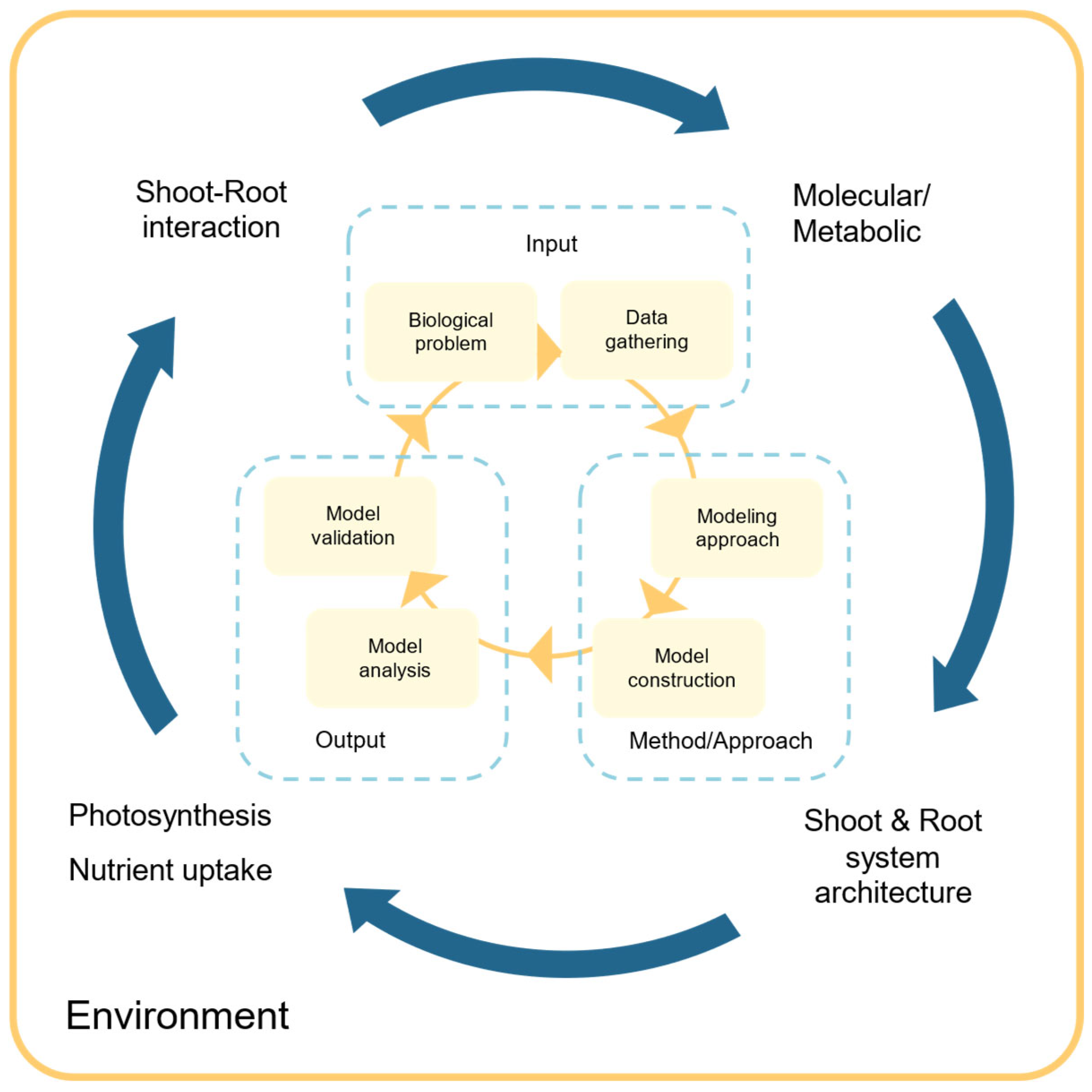
Figure 2.
A proposed workflow for modelling metabolism. We subdivide the workflow into input, method/approach, and output. The input illustrates necessary a priori details for building a metabolic model. These details include data collection, pathway reconstruction, and stoichiometric matrix calculation. In the second step, the method/approach compartment illustrates the process for FBA, kinetic, and hybrid model building. The final step is the output compartment, where we represent the possible results from each of the different approaches, together with types of analysis that can be performed.
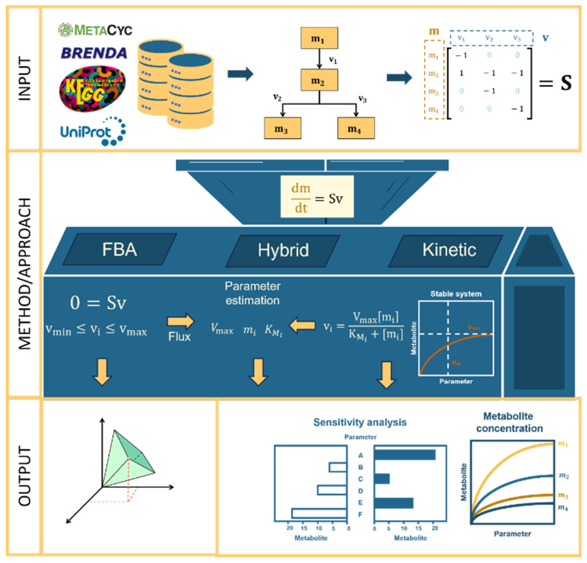
Figure 3.
Proposed workflow for modeling shoot and root system architectures. The input panel includes determining whether the plant species to model is a monocot or dicot. The method panel presents the basic modeling unit, which we either stack up or iterate to form the full architecture. The output panel gives the quantified traits of the shoot and root architecture.
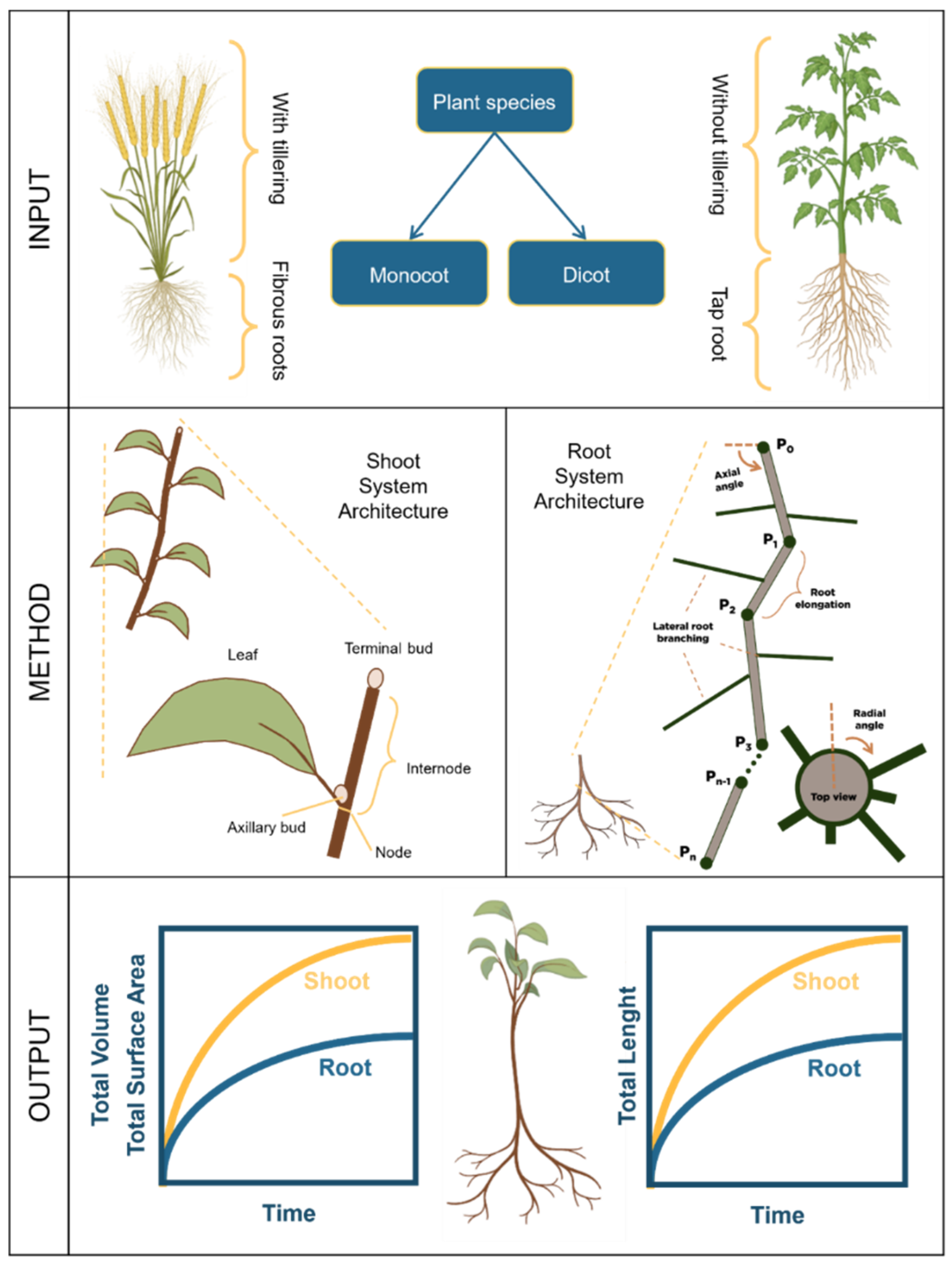
Figure 4.
Proposed workflow for modeling resource acquisition. Shoot photosynthesis and root nutrient uptake models need to be integrated. The input panel splits into acquisition of light and in the shoot and acquisition of mineral nutrients in the root. The methods panel summarizes available methods to build each type of models. The output panel illustrates shoot and root resource acquisition traits that can be quantified using the models.
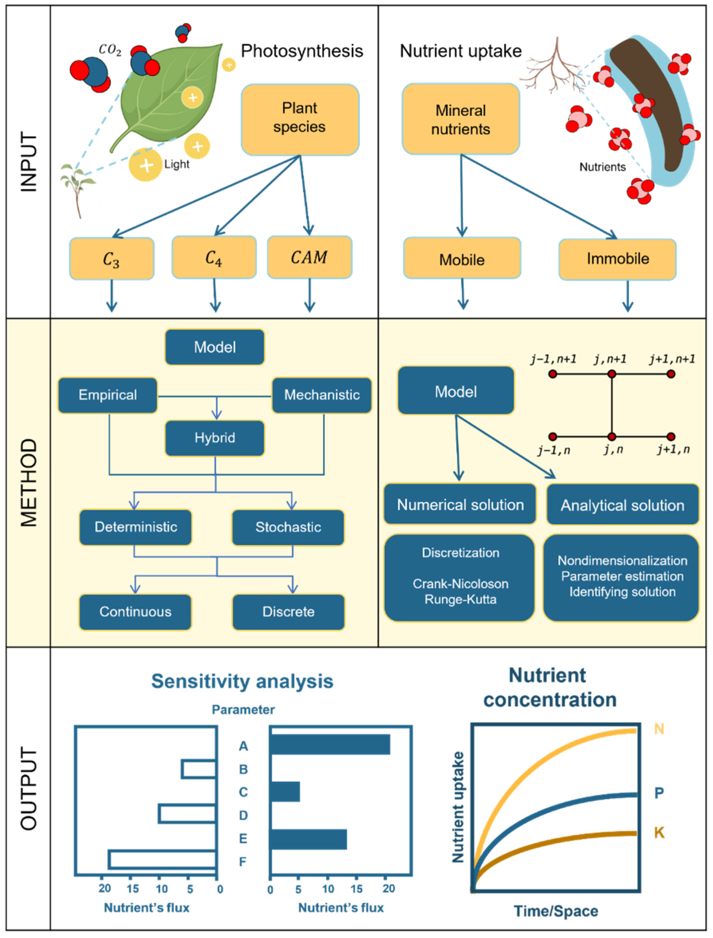
Figure 5.
Proposed workflow for modeling shoot-root interaction.
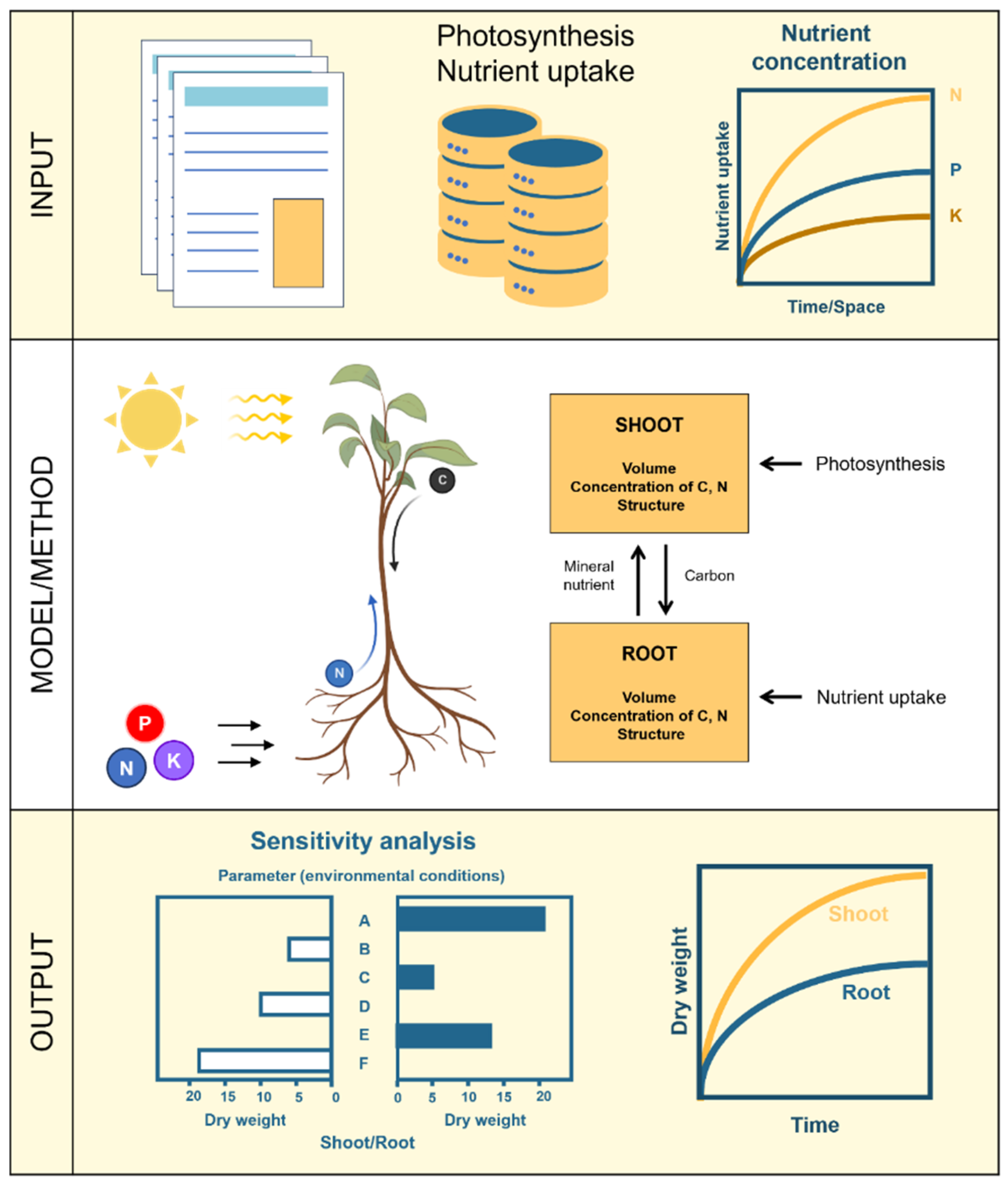
Disclaimer/Publisher’s Note: The statements, opinions and data contained in all publications are solely those of the individual author(s) and contributor(s) and not of MDPI and/or the editor(s). MDPI and/or the editor(s) disclaim responsibility for any injury to people or property resulting from any ideas, methods, instructions or products referred to in the content. |
© 2024 by the authors. Licensee MDPI, Basel, Switzerland. This article is an open access article distributed under the terms and conditions of the Creative Commons Attribution (CC BY) license (http://creativecommons.org/licenses/by/4.0/).
Copyright: This open access article is published under a Creative Commons CC BY 4.0 license, which permit the free download, distribution, and reuse, provided that the author and preprint are cited in any reuse.


