
Submitted:
21 October 2024
Posted:
22 October 2024
You are already at the latest version
Abstract
The effects of neighboring transitions (ENT) on electromagnetically induced transparency (EIT), electromagnetically induced absorption (EIA), and the conversion between EIA and EIT in a degenerate multi-level system of 87Rb atoms were studied in terms of the angle (θ) between the polarization axes of the coupling and probe beams. The predicted critical values of θ, in which EIT transitioned to EIA, were consistent with the experimental values. In this work these results were systematically confirmed using the calculated spectra by varying the frequency spacings in the excited state of 87Rb via a factor called the ratio. We observed that when the ratio was less than 0.1, the critical angle θc was inverted. This may be attributed to the interplay between the strengths of the EIA and EIT as the ENT varied. We also discovered that by modifying the frequency spacings in the excited state of 87Rb, it becomes feasible to predict ENT and the interplay between EIT and EIA in alkali-metal atoms.
Keywords:
EIA
; EIT
; Rubidium
1. Introduction
Converting between electromagnetically induced absorption (EIA) and electromagnetically induced transparency (EIT) allows the sign of the dispersion slope to be manipulated, which provides exceptional control over the properties of the medium in a coherent manner. However, many studies on how the polarizations [1,2,3,4] of the probe and coupling beams depend on the conversion between EIT and EIA have not considered the effects of the neighboring transitions (ENT).
The conversion between the EIA and EIT can be controlled in many ways [5,6,7,8,9,10,11,12,13,14]. Reversing the sign of EIT with respect to the polarization ellipticity for the transition of 87Rb has been investigated without accounting for ENT [15,16,17,18,19]. However, the total absorption of the D2 line incorporating the Doppler effect could not be determined [13]. Gozzini et al. [1] confirmed that the EIT can be tuned continuously to the EIA by choosing right-handedness of the circular polarization and appropriate propagation direction of the coupling and probe beams.
In addition, a theoretical model for a graphene metastructure featuring switchable properties between EIT and EIA within a three-resonator system has been developed [10]. Chanu et al. [14] showed that an N-type formation using two control beams enabled to the conversion from EIT to EIA. Depending on the various polarization combinations, EIT or EIA can be formed such that it is possible to make a convert between EIA and EIT. Moreover, the angle dependence of the polarization axes of the coupling and probe beams on EIA and EIT in 85Rb atoms caused by ENT [20] (in which EIT or EIA can occur) has been reported. However, the switching mechanism for alkali-metal atoms is still not well known. The ENT in adjacent multi-level systems, combined with a change in the angles between the polarization axes of the coupling and probe beams, is important in the mechanisms that convert between EIT and EIA.
In this study the ENT and angle between the polarization axes of the coupling and probe beams in the transitions of 87Rb are investigated. The critical angle was measured and calculated in cases in which EIT could be converted into EIA. We also found that the ENT can be derived from the critical angles obtained by artificially varying the spacings of the excited states of 87Rb because the conversion between EIA and EIT strongly depends on the ENT. We also found that by adjusting the frequency spacings in the excited state of 87Rb, it becomes possible to predict ENT and the competition between EIT and EIA in alkali-metal atoms including 87Rb atom.
2. Theoretical Calculation
The energy level diagram for 87Rb is shown in Figure 1, in which the blue (red) arrow and “0” (“”) represent the transitions excited by the coupling (probe) beam and its relative frequency, respectively ( is defined below). To examine the ENT in the EIA or EIT spectra, we intentionally varied the frequency spacings in the excited state. In this case, the frequency spacings shown in Figure 1 vary by a common factor defined as the ratio (see Figure 7 in Section 5).
Both the coupling and probe beams were linearly polarized, and their polarization axes differed by an angle . Because the power of the coupling beam was larger than that of the probe beam by a factor of 3.3 in the experiment, we selected the polarization axis of the coupling beam as the quantization axis. Selecting the polarization axis of the probe beam as the quantization axis is also possible, but in this case, we need to use higher interactions than the three photons, normally used in the calculation, can provide to guarantee sufficient accuracy. In the spherical bases, the polarization axes of the coupling and probe beams are given by and , respectively, where
Therefore, the coupling beam excited the transitions with , whereas the probe beam excites the transitions with and , as shown in Figure 1.
The density matrix equation for the , and 3 transitions of the 87Rb D2 line is given by
where is the density operator, is the term associated with the relaxation phenomena [21]. The Hamiltonian (H) in Equation (2) is expressed as
where , , () is the detuning of the coupling (probe) beam, k is the wave vector, v is the velocity of an atom, and is the frequency spacing between the states and . In Equation (3), () is the Rabi frequency of the probe (coupling) beam, h.c. represents the Hermitian conjugate, and is the normalized transition strength between the states and [22].
The density matrix elements should be expanded into several terms that oscillate at different oscillation frequencies. The expansions of the density matrix elements between the excited and ground states, the excited and excited states (and the ground and ground states), and the populations are given by Eqs. (5)–(7) and Eqs. (8) and (9), and Eq. (10) in [20], respectively
A series of coupled time-dependent differential equations, obtained by inserting the Hamiltonians and expanded density matrix elements into Equation (2), was solved for the steady-state regime. Then, the final absorption coefficient, averaged over the Maxwell–Boltzmann velocity distribution, is given by
where is the wavelength of the laser, is the most probable speed of the atoms, and is the atomic density in the cell. is the decomposed matrix element of oscillating as . To perform a quantitative analysis of the ENT on the spectra, we performed two types of calculations: degenerate two-level system (DTLS) calculation and degenerate multi-level system (DMLS) calculation. In the DMLS (DTLS) calculation, all neighboring hyperfine states were taken into account (neglected).
3. Experimental Setup
A laser beam with wavelength of 780 nm from a tunable external cavity diode laser (DLpro, Toptica Inc.) was transmitted through an optical window; a small portion of the laser beam was reflected for saturated absorption spectroscopy, and the rest was sent to a polarizing beam splitter (PBS-1), as shown in Figure 2. A half-wave plate (HWP) was placed before PBS-1 to divide the beam into coupling and probe beams and to maintain the beam power ratio between the two resulting beams. The probe beam was expanded by 5–6 mm in diameter using a beam expander (GBE05-B, Thorlabs), and the beam was aimed at the vapor cell after it passed through the beam splitter (BS). The HWP placed before the BS maintained the polarization of the probe beam. The vapor cell was 5 cm in length and 2.5 cm in diameter. The vapor cell is protected from the effects of stray magnetic fields and Earth’s magnetic field by five layers of -metal sheet. The coupling beam was scanned by passing it through two acousto-optic modulators (AOM). The first AOM, labeled AOM-1 (3080-122, Gooch & Housego) was fixed at 80 MHz using the AOM driver (1080AF-AINA-1.0 HCR, Gooch & Housego), and the other AOM, labeled AOM-2 (3080-122, Crystal Technology, Inc.), was scanned within MHz at MHz using the deflector driver (DE-802EM26, IntraAction). To match the polarization of the probe beam (P-polarized), another set of HWPs and PBSs were used for the coupling beam. A beam expander (GBE05-B, Thorlabs) was used to expand the coupling beam to a diameter of 6 mm. Both the probe and coupling beams met at the BS;to specify , and the HWP was placed in the path of the coupling beam before it reached the BS. For 10 different settings of HWPs placed before the BS, spectral profiles were recorded for the and 3 transitions of 87Rb.
4. Experimental and Calculated Results
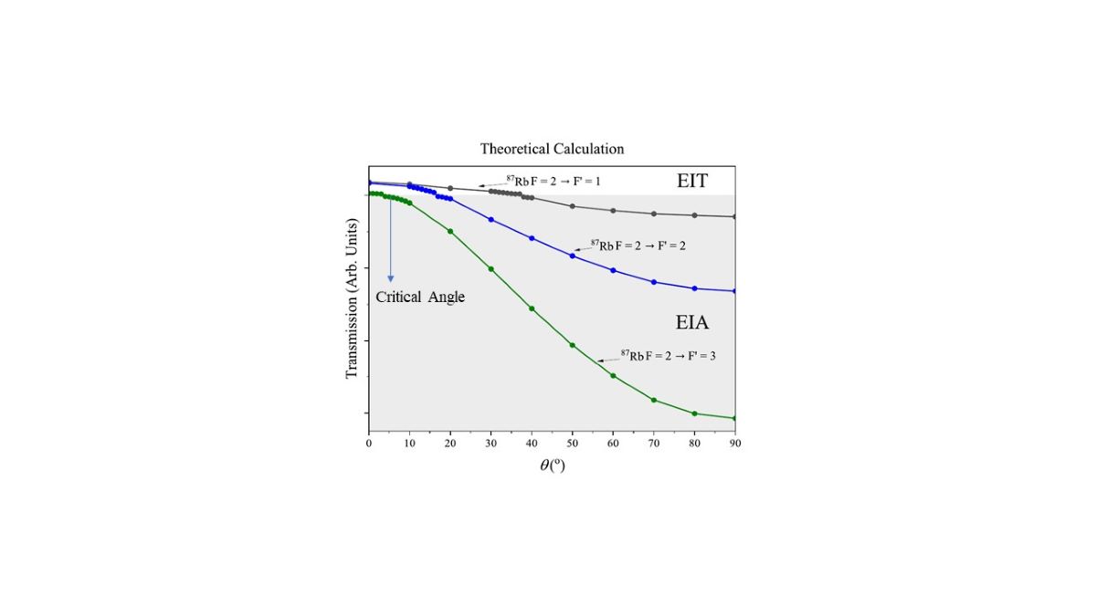
The calculated spectra for the DTLS and DMLS and the experimental spectra for the transitions from the upper-ground hyperfine energy level F = 2 of the D2 line of 87Rb are shown in Figure 3, Figure 4 and Figure 5, respectively. The closed transition exhibited EIT instead of EIA at . However, the open and transitions exhibited EIAs at larger , as shown in Figure 3c, Figure 4c, and Figure 5c.
The calculated spectra for the DTLS and DMLS and experimental spectra for the closed = 3 transition are shown in Figure 3a–c, respectively. Instead of EIA, EIT appeared at . The EIT switched to EIA at . After the switch to EIA, the amplitudes of the EIA increased as increased. The maximum EIA amplitude appeared at , as shown in Figure 3c. The experimental spectra were consistent with the calculated spectra for the DMLS, as shown in Figure 3b, with EIT at . The influence of the open = 2 and = 1 transitions resulted in EIT at . This was why the calculated spectra for the DTLS that neglected the contributions from neighboring transitions for the closed = 3 transition had EIAs at all , as shown in Figure 3a. The calculated EIA spectra for the DTLS also increased in amplitude as increased.
For the open transition, the amplitudes of the EIT increased as increased for the DTLS calculation with relatively small amplitudes, as shown in Figure 4a. Because of the dominance of the closed = 3 transition, the calculated EIT spectra for the DMLS switched to EIA at , as shown in Figure 4b. Similarly, the experimental spectra shown in Figure 4c reflect the conversion of EIT to EIA. After switching, the EIA amplitude increased as increased, and the maximum amplitude occurred at . The EIT, in contrast, had a maximum amplitude at for both calculated spectra for the DMLS and experimental spectra.
For the transition, the amplitude of the EIT increased as increased for the calculated spectra for the DTLS, as shown in Figure 5a. This transition is further away from the transition because hyperfine splitting was large, which was why the EIT switched to EIA at a larger compared to the transition for the calculated spectra for the DMLS shown in Figure 5b. The EIT switched to EIA at a larger angle, as shown in Figure 5c, and was not consistent with the DMLS spectra. A plausible reason for this discrepancy is given in Section 5 using a small variation of the transmission at .
5. Discussion
To accurately determine the critical , the line-center transmission with respect to the transmission of the broad spectrum was plotted as a function of . The experimental and calculated results are shown in Figure 6a,b, respectively. The experimental values of the critical angle for the , and 1 transitions were measured to be , , and , respectively. To accurately determine the theoretical critical , a interval near the critical angle was used instead of a interval. The calculated values were , , and , respectively. Thus, the experimental and calculated results were in good agreement, except for the transition. In the experiment, the line-center transmission values gradually increased as increased, and this trend was also observed in the calculated results. The experimental line-center transmission of the transition line deviated from the theoretical expectation. This discrepancy can be explained as follows: as is readily seen in Figure 6b, the variation in the transmission at for the transition was very small compared to those for the transitions. Thus, the critical angle may have been inaccurately determined.
The critical angles displayed in Figure 7 show the strength of the ENTs in the EIA and EIT spectra. Compared to the results for 85Rb reported in [20], the critical angles for the transitions of 87Rb were larger than those of 85Rb, and vice versa for the transition. In this work to investigate this phenomenon more systematically, we calculated the critical angles by intentionally varying the frequency spacings in the excited state of 87Rb using a factor called the ratio. For example, if the ratio was unity, the critical angles corresponded to the values for pure 87Rb, as shown in Figure 7. In contrast, if the ratio was to 0.5, the frequency spacings were reduced to half that of 87Rb. In this case, the neighboring effect increased compared to the case of 87Rb.
Figure 7.
Critical angles () versus the strength of the ENT on the EIA and EIT spectra.
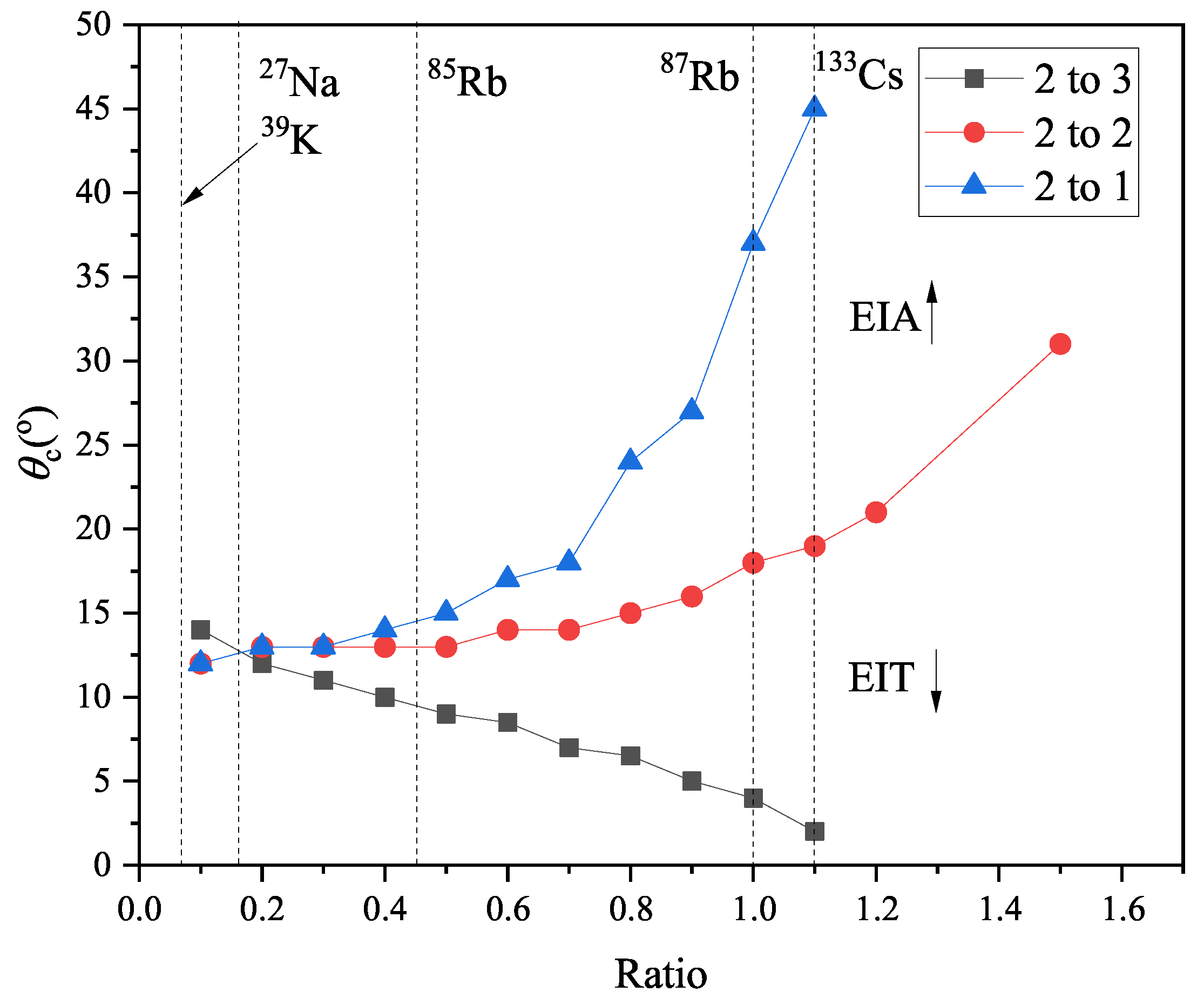
The calculated results are presented in Figure 7. The critical angles for the , and 3 transitions are displayed from top to bottom as a function of the ratio. As the ratio increased, the critical angles for the transitions ( transition) increased (decreased) monotonically. The calculation of was not accurate, unlike in typical critical phenomena. This occurred because, when the EIT was converted into the EIA, the introduction of the EIA was gradual rather than radical. However, because our aim was to determine only the overall trend of the transmissions, an inaccurate determination of did not impact the results of this study.
Because the conversion between the EIA and EIT strongly depends on the ENT rather than the energy level structure, the behavior of other atomic species can be easily predicted by changing the frequency spacings. More accurately, the ENT depends on the frequency spacing divided by the natural linewidth of the transition, which is regarded as the effective frequency spacing. In Figure 7 the values are presented as vertical dotted lines. For example, the critical angles for 133Cs were larger (smaller) for the transitions ( transition) than those for 87Rb. We expect that the conversion between EIA and EIT occurs for other atomic species in a similar way.
For the transition, as changed from 0 to , the strong transitions between the and states began to produce the EIA signal. The EIT was converted to the EIA at . If the ratio was decreased (i.e., the ENT was increased) while was fixed at , then the effect of the transition on the transition increased, and the signal changed to EIT accordingly. Thus, increased as the ratio decreased as shown in Figure 7.
For the and transitions, the conversion from EIT to EIA occurred at a larger value of because of the off-resonant contribution of the strong transition. In this case, as the ratio decreased (i.e. as the ENT increased), the signal changed to EIA owing to the effect of the transition. Thus, decreased as the ratio decreases, in contrast to the case of the transition.
For the transition, only the EIA could be observed when the ratio was larger than approximately 1.2. In this case, the ENT was not sufficient to convert EIA into EIT. When the ratio was very large, which corresponded to the case in which the ENT was absent, only the EIA for the transition and the EIT for the and transitions could be observed. This corresponded exactly to the calculation for the DTLS.
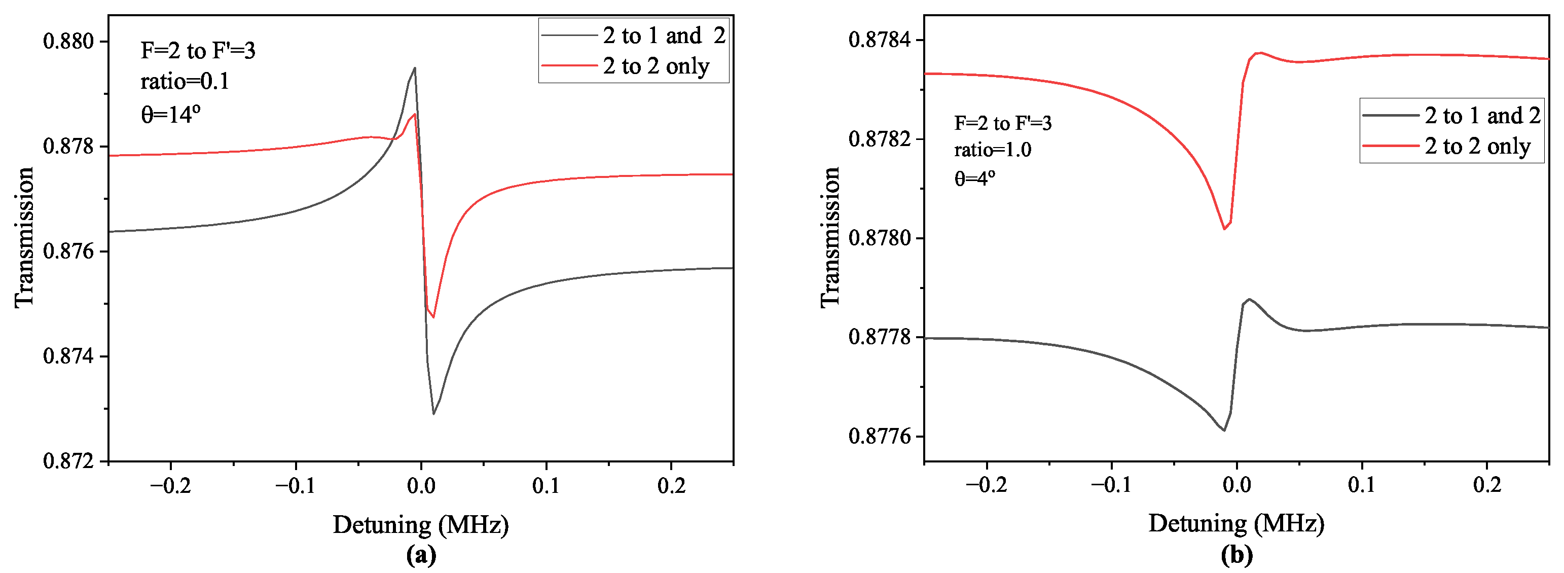
In Figure 7, the inversion of can be observed for ratio values smaller than approximately 0.1, (i.e., a larger was observed for the transition than the transitions.) This phenomenon may have resulted from the interplay between the strength of the EIA owing to the transitions between the and states and that of the EIT owing to the transitions when the ENT increased. To examine this phenomenon more quantitatively, we calculated the spectra for the transition when the ratios were and accounting for all the ENT and excluding the effect of the transition.
The results for the ratios of and at are shown in Figure 8a,b, respectively. In Figure 8, the black curves represent the spectra accounted for all the neighboring transitions and the red curves represent the spectra that considered only the transition (i.e., neglected the transition). The angles were and , as shown in Figure 8a,b, respectively. In Figure 8a, the strengths of the EIT and EIA were comparable for the black curve, and the effect of the EIT was weaker than that of the EIA for the red curve. In contrast, as shown in Figure 8b, the effect of the transition was very weak because of the larger hyperfine spacing. Thus, when the ratio was , the effect of the EIT was enhanced owing to the neighboring transitions associated with the EIT, and a larger needed to be converted from EIT to EIA. Thus, we could observe larger for the transition when the ratio was smaller than approximately .
6. Conclusions
In this study, the ENT on EIA, EIT, and the conversion between EIA and EIT in 87Rb atoms were investigated in terms of the angle between the polarization axes of the coupling and probe beams. The observed spectral profiles were compared to the calculated absorption profiles by considering the ENT. The results were consistent with the observed spectra for all the transitions. The slight quantitative disagreement for the transition was explained by accounting for the weak variation in the transmission for .
EIT (instead of EIA) occurred at smaller for the upper hyperfine ground state of 87Rb, and the amplitude of the EIA increased as increased for all the and 3 transitions after the transformation from EIT to EIA. The theoretical critical , at which EIT is converted to EIA, was consistent with the experimentally measured critical values except for the transition. Compared to 85Rb, the critical angles for the transitions in 87Rb were greater, whereas for the transition, the critical angles were smaller. We observed an inversion of the critical angle when the ratio was smaller than 0.1, resulting in a larger for the transition compared to the and transitions. This phenomenon was explained by accounting for the competition between the strengths of the EIA and EIT as the ENT varied. The results of this study can deepen our understanding of the ENT on EIA and EIT spectra, and can support useful predictions of the spectra for alkali-metal atoms other than 87Rb atoms.
Author Contributions
Conceptualization, J.K. and H.N.; methodology, A. H.; formal analysis, J.K. and H.N.; investigation, A. H., J. K., H. N..; writing—original draft preparation, A. H., J. K., H. N.; writing—review and editing, J. K., H. N.; supervision, J. K.; project administration, J. K., H. N.; funding acquisition, J. K., H. N.
Funding
This work was supported by the National Research Foundation of Korea (NRF) grant funded by the Korean government (MSIT) (Nos. 2020R1A2C1005499 and RS-2023-00239275).
Institutional Review Board Statement
Not applicable.
Informed Consent Statement
Not applicable.
Data Availability Statement
Not applicable.
Acknowledgments
This work was supported by the National Research Foundation of Korea (NRF) grant funded by the Korean government (MSIT) (Nos. 2020R1A2C1005499 and RS-2023-00239275).
Conflicts of Interest
The authors declare no conflicts of interest.
References
- Gozzini, S.; Fioretti, A.; Lucchesini, A.; Marmugi, L.; Marinelli, C.; Tsvetkov, S.; Gateva, S.; Cartaleva, S. Tunable and polarization-controlled high-contrast bright and dark coherent resonances in potassium. Opt. Lett. 2017, 42, 2930–2933. [Google Scholar] [CrossRef] [PubMed]
- Molella, L.S.; Dahl, K.; Rinkleff, R.-H.; Danzmann, K. Coupling-probe laser spectroscopy of degenerate two-level systems: An experimental survey of various polarisation combinations. Opt. Commun. 2009, 282, 3481–3486. [Google Scholar] [CrossRef]
- McGloin, D.; Dunn, M.H.; Fulton, D.J. Polarization effects in electromagnetically induced transparency. Phys. Rev. A 2000, 62, 053802. [Google Scholar] [CrossRef]
- Ram, N.; Pattabiraman, M. Sign reversal of Hanle electromagnetically induced absorption with orthogonal circularly polarized optical fields. J. Phys. B: At. Mol. Opt. Phys. 2010, 43, 245503. [Google Scholar] [CrossRef]
- Gao, C.J.; Zhang, H.F. Switchable Metasurface with Electromagnetically Induced Transparency and Absorption Simultaneously Realizing Circular Polarization-Insensitive Circular-to-Linear Polarization Conversion. J. Ann. Phys. 2022, 534, 2200108–220013. [Google Scholar] [CrossRef]
- Lv, Y.; Zhu, D.-D.; Sun, Y.-Z.; Zhang, D.; Zhang, H.-F. Transition from electromagnetically induced transparency to electromagnetically induced absorption utilizing phase-change material vanadium dioxide based on circularly polarized waves. Physica E: Low dimensional systems and nanostructure 2023, 145, 115507–115526. [Google Scholar] [CrossRef]
- Yu, H.; Kim, J.D.; Jung, T.Y.; Kim, J.B. Transformation of EIA to EIT by incoherent pumping of the 85Rb D1 line. J. Kor. Phys. Soc. 2012, 61, 1227–1231. [Google Scholar] [CrossRef]
- Bhattarai, M.; Bharti, V.; Natarajan, V. Tuning of the Hanle effect from EIT to EIA using spatially separated probe and control beams. Sci. Rep. 2018, 8, 7525. [Google Scholar] [CrossRef]
- Yin, Y.; Lv, Y.; Sun, Y.; Zhang, H. Tunable conversion of electromagnetically induced transparency to electromagnetically induced absorption based on vanadium dioxide metastructure. Optik 2024, 296, 171554–171560. [Google Scholar] [CrossRef]
- Zhu, D.-D.; Lv, Y.; Sun, Y.-Z.; Zhang, H.-F. Switching of electromagnetically induced transparency and absorption of graphene metastructure with the three resonators. Waves in Random and Complex Media 2023, 0, 1–25. [Google Scholar] [CrossRef]
- Bae, I.-H.; Moon, H.S.; Kim, M.-K.; Lee, L.; Kim, J.B. Transformation of electromagnetically induced transparency into enhanced absorption with a standing-wave coupling field in an Rb vapor cell. Opt. Express 2010, 18, 1389–1397. [Google Scholar] [CrossRef] [PubMed]
- Yi, C.-J.; Shen, M.-C.; Qin, Q.; Zhang, Y.-F.; Lin, X.-M.; Ye, M.-Y. Transition from electromagnetically-induced transparency to absorption in a single microresonator. Opt. Express 2023, 31, 7167–7174. [Google Scholar] [CrossRef] [PubMed]
- Grewal, R.S.; Pattabiraman, M. Hanle electromagnetically induced absorption in open Fg→Fe≤Fg transit ions of the 87Rb D2 line. J. Phys. B: At. Mol. Opt. Phys. 2015, 48, 085501. [Google Scholar] [CrossRef]
- Chanu, S.R.; Pandey, K.; Natarajan, V. Conversion between electromagnetically induced transparency and absorption in a three-level lambda system. Europhys. Lett. 2012, 98, 44009. [Google Scholar] [CrossRef]
- Jadoon, Z.A.S.; Noh, H.R.; Kim, J.T. Effects of neighboring transitions on the mechanisms of electromagnetically induced absorption and transparency in an open degenerate multilevel system. Sci. Rep. 2022, 12, 145. [Google Scholar] [CrossRef]
- Jadoon, Z.A.S.; Hassan, A.-u.; Noh, H.R.; Kim, J.T. Effects of neighboring transitions on electromagnetically induced absorption and transparency in 85Rb atoms based on the linear parallel polarization of coupling and probe beams. Opt. Commun. 2022, 520, 128512. [Google Scholar] [CrossRef]
- Jadoon, Z.A.S.; Hassan, A.-u.; Noh, H.R.; Kim, J.T. Electromagnetically induced absorption in Rb atoms with circular polarization of laser beams: Effects of neighboring transitions. Heliyon 2022, 8, 11752. [Google Scholar] [CrossRef]
- Hassan, A.-u.; Jadoon, Z.A.S.; Noh, H.R.; Kim, J.T. Effects of neighboring transitions on electromagnetically induced absorption and transparency in Rb atoms in circular orthogonal polarization configuration. J. Kor. Phys. Soc. 2023, 82, 907–911. [Google Scholar] [CrossRef]
- Jadoon, Z.A.S.; Hassan, A.-u.; Noh, H.R.; Kim, J.T. Effects of neighboring transitions on electromagnetically induced absorption and transparency in 87Rb atoms with respect to varying hyperfine spacings. J. Opt. Soc. Am. B 2023, 40, 2612–2617. [Google Scholar] [CrossRef]
- Hassan, A.-u.; Noh, H.-R.; Kim, J.T. Angle dependence between the polarization axes of the coupling and probe beams on electromagnetically induced absorption and transparency in 85Rb atoms due to neighboring effect. Optik 2024, 311, 171906. [Google Scholar] [CrossRef]
- Choi, G.W.; Noh, H.R. Line shapes in sub-Doppler DAVLL in the 87Rb-D2 line. Opt. Commun. 2016, 367, 312–315. [Google Scholar] [CrossRef]
- Choi, G.W.; Noh, H.R. Sub-Doppler DAVLL spectra of the D1 line of rubidium: a theoretical and experimental study. J. Phys. B: At. Mol. Opt. Phys. 2015, 48, 115008. [Google Scholar] [CrossRef]
Figure 1.
Energy level diagram for the and 3 transitions of the 87Rb D2 line. The blue and red lines indicate the transitions excited by the coupling and probe beams, respectively.
Figure 1.
Energy level diagram for the and 3 transitions of the 87Rb D2 line. The blue and red lines indicate the transitions excited by the coupling and probe beams, respectively.
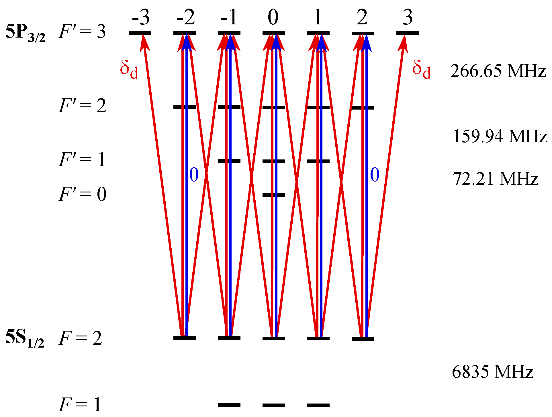
Figure 2.
Schematic of the experimental setup. SAS: saturated absorption spectroscopy; W: window; HWP: half-wave plate; PBS: polarizing beam splitter; BE: beam expander; AOM: acousto-optic modulator; M: mirror; BS: beam splitter; Bd: beam dump; PD: photodetector.
Figure 2.
Schematic of the experimental setup. SAS: saturated absorption spectroscopy; W: window; HWP: half-wave plate; PBS: polarizing beam splitter; BE: beam expander; AOM: acousto-optic modulator; M: mirror; BS: beam splitter; Bd: beam dump; PD: photodetector.
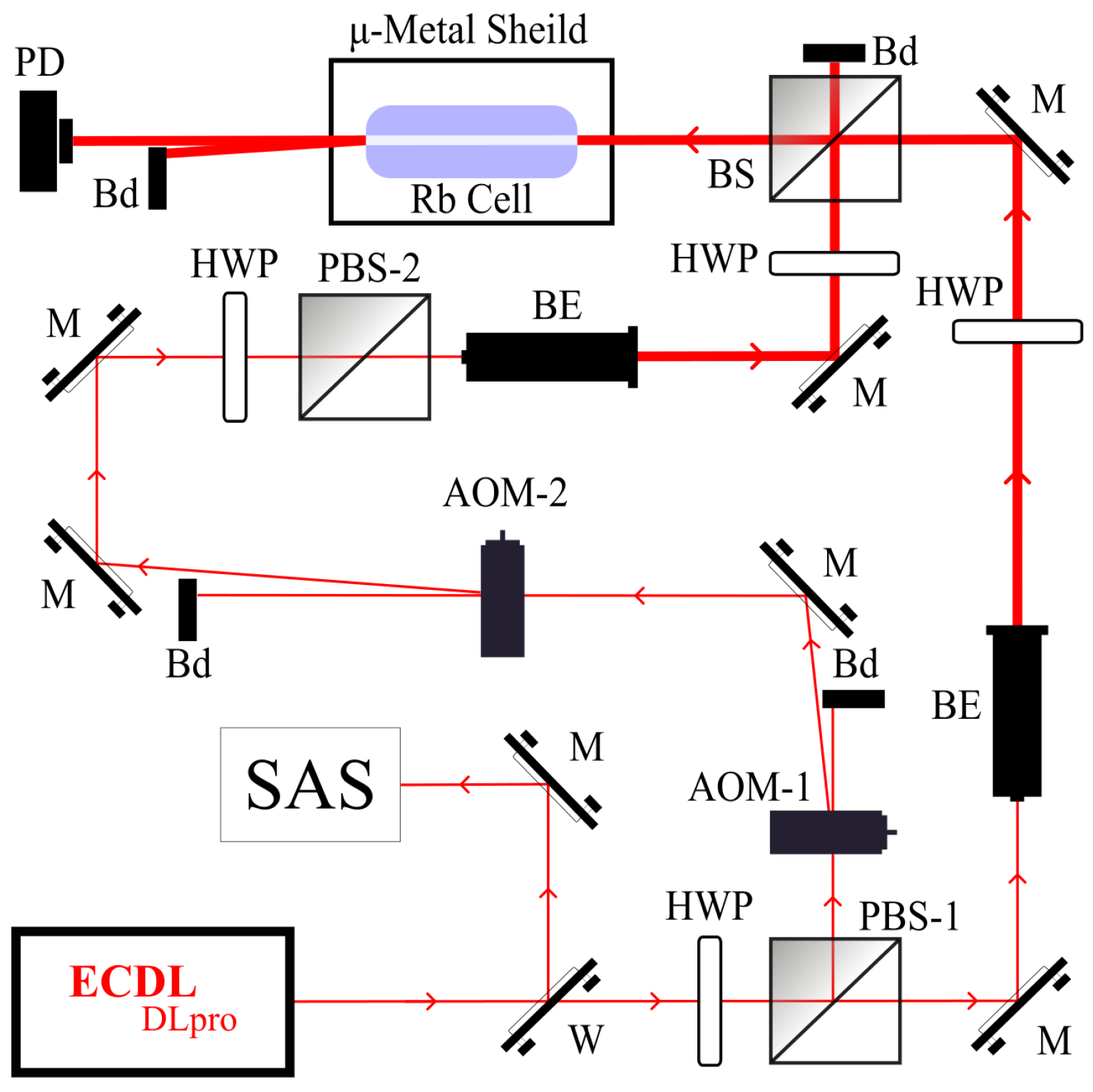
Figure 3.
Calculated spectra for the (a) DTLS (b) DMLS, and (c) experimentally measured spectra for the resonant transition.
Figure 3.
Calculated spectra for the (a) DTLS (b) DMLS, and (c) experimentally measured spectra for the resonant transition.
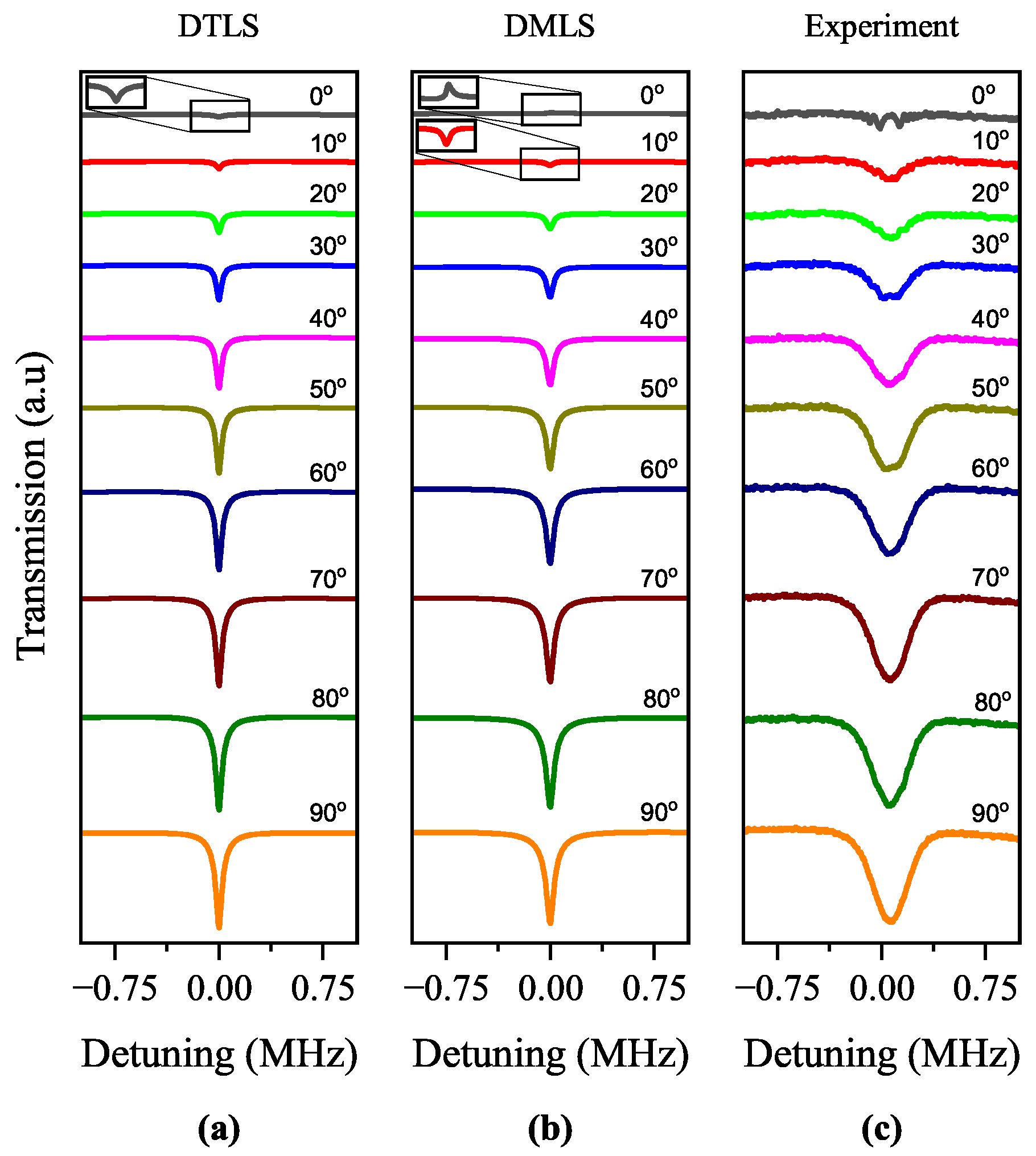
Figure 4.
Calculated spectra for the (a) DTLS (b) DMLS, and (c) experimentally measured spectra for the resonant transition.
Figure 4.
Calculated spectra for the (a) DTLS (b) DMLS, and (c) experimentally measured spectra for the resonant transition.
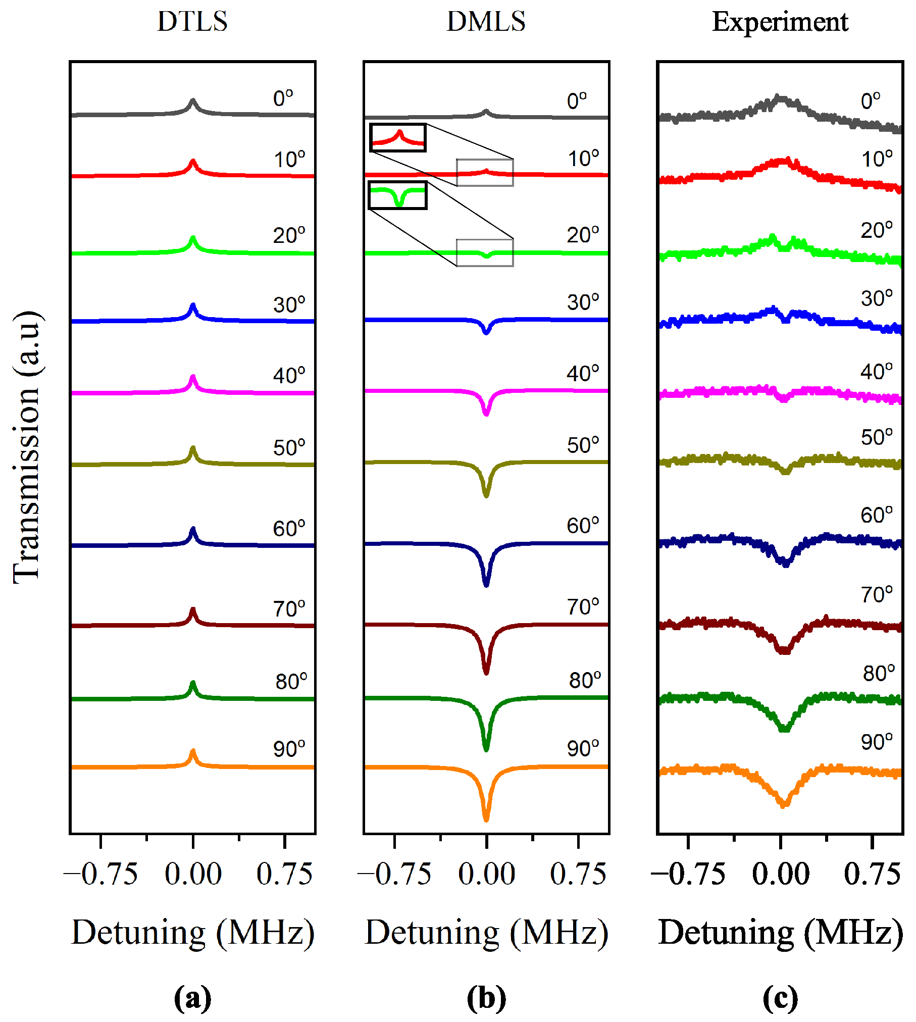
Figure 5.
Calculated spectra for the (a) DTLS (b) DMLS, and (c) experimentally measured spectra for the resonant transition.
Figure 5.
Calculated spectra for the (a) DTLS (b) DMLS, and (c) experimentally measured spectra for the resonant transition.
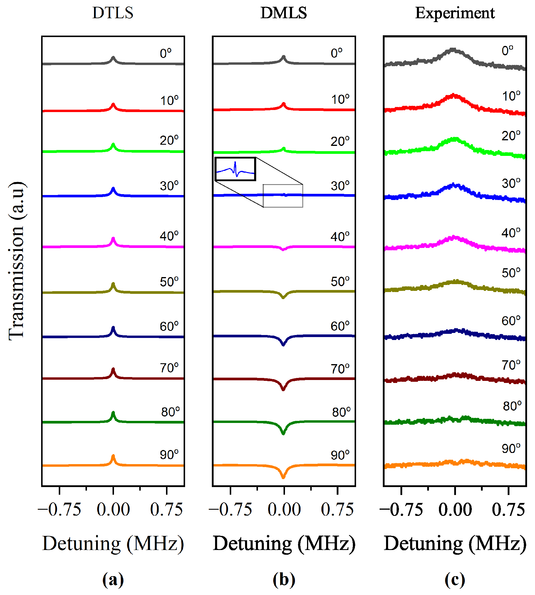
Figure 6.
(a) Experimental and (b) theoretical line–center transmission values with respect to for the = 1, 2, and 3 transitions.
Figure 6.
(a) Experimental and (b) theoretical line–center transmission values with respect to for the = 1, 2, and 3 transitions.
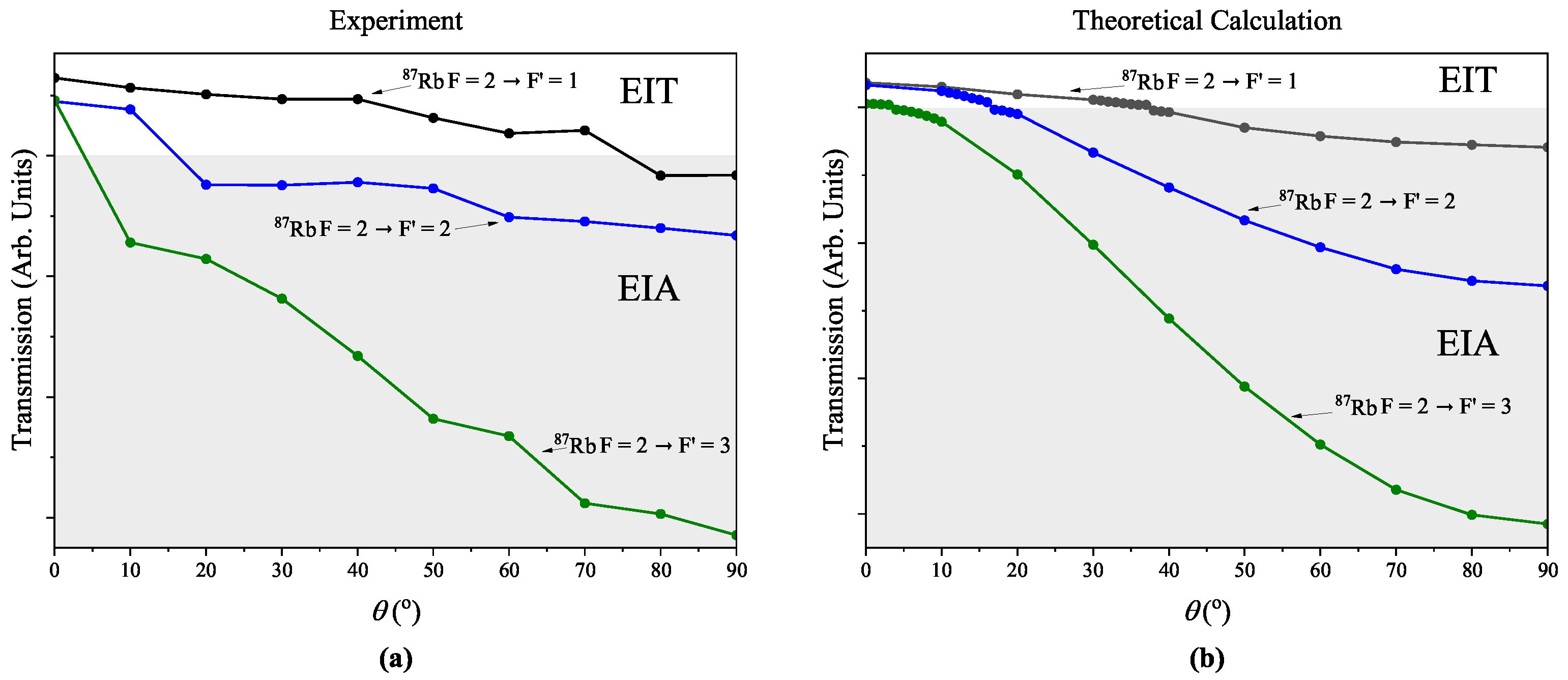
Figure 8.
The spectral results for the ratio of (a) with and (b) with for the transition. The black curves represent the spectra that accounted for all the neighboring transitions and the red curves represent the spectra that considered only the transition.
Figure 8.
The spectral results for the ratio of (a) with and (b) with for the transition. The black curves represent the spectra that accounted for all the neighboring transitions and the red curves represent the spectra that considered only the transition.
Disclaimer/Publisher’s Note: The statements, opinions and data contained in all publications are solely those of the individual author(s) and contributor(s) and not of MDPI and/or the editor(s). MDPI and/or the editor(s) disclaim responsibility for any injury to people or property resulting from any ideas, methods, instructions or products referred to in the content. |
© 2024 by the authors. Licensee MDPI, Basel, Switzerland. This article is an open access article distributed under the terms and conditions of the Creative Commons Attribution (CC BY) license (http://creativecommons.org/licenses/by/4.0/).
Copyright: This open access article is published under a Creative Commons CC BY 4.0 license, which permit the free download, distribution, and reuse, provided that the author and preprint are cited in any reuse.


