
Submitted:
25 September 2025
Posted:
25 September 2025
You are already at the latest version
Abstract
Earlier quantum calculations of the optical response of Nakamura’s blue laser diode, assuming Kronig–Penney-like band-edge profiles, omitted the effects of charge polarization, cladding-layer asymmetry, and recombination delay times. While such simplified model reproduces the overall emission structure, underestimates the spectral width and fails to capture the decrease in peak intensities at higher energies. Here, we present a detailed quantum theory of polarized-asymmetric superlattices that explicitly incorporates spontaneous and piezoelectric polarization, confining-layer asymmetry, and recombination lifetimes. Local Stark fields are modeled by linear band-edge potentials, and the corresponding Schrödinger equation is solved using Airy functions within the Theory of Finite Periodic Systems. This approach enables the exact calculation of subband eigenvalues, eigenfunctions, transition probabilities and optical spectra. We show that to faithfully reproduce Nakamura’s blue laser spectra, smaller effective masses must be considered, unless unrealistically small barrier heights and widths are assumed. Furthermore, by employing the time distribution of transition probabilities, we capture the energy dependence of recombination lifetimes and their influence on peak intensities. The resulting analysis reproduces the observed spectral broadening and peak-height evolution, while also providing estimates of the magnitude of the Stark effect and mean recombination lifetimes.
Keywords:
Blue laser diode spectra
; InGaN superlattices
; Quantum theory of polarized superlattices
; Quantum-confined Stark effect (QCSE)
; Charge polarization
; Confining-layers asymmetry
; Recombination delay times
; Optical susceptibility
1. Introduction
The discovery in the 1990s of blue laser diodes based on N superlattices in the active region [1,2] triggered rapid progress in solid-state lighting, optoelectronics, and related technologies. Since then, intensive efforts have been devoted to improve epitaxial growth, structural quality, and device performance of GaN-based heterostructures and superlattices (SLs)[3,4,5,6,7,8,9,10,11]. Subsequent research concentrated on Ga-rich InGaN and AlGaN alloys, whose bandgaps enable photon emission across the blue–green spectral range [12,13].
Despite extensive work on carrier transport, effective masses, device efficiency, and brightness, the detailed optical response of InGaN/GaN superlattice diodes has received comparatively less attention. High-resolution spectra reveal groups of narrow emission peaks, but their theoretical explanation has long been regarded as overly demanding due to the quantum-mechanical complexity of the problem. In particular, interpreting the spectra first reported in Nakamura’s pioneering experiments has remained a challenge. Several theoretical and experimental studies have addressed partial aspects of the emission process. Examples include the joint density-of-states model for multi-quantum-well heterostructures [14] and works comparing polar and non-polar quantum wells, which showed that structural non-uniformity broadens optical transitions [15]. Conventional approaches based on effective-mass and models, however, rely implicitly on Bloch’s theorem, which is rigorously valid only for infinite crystals. For finite periodic systems such as superlattices, Bloch-based descriptions become inadequate: they replace a quantum-discrete spectrum with a classical continuum approximation, and in doing so eliminate precisely the discrete features observed experimentally.
In the 1980s, several independent works [35] applied the transfer-matrix method to multilayered structures and, without apparent knowledge of earlier studies, effectively rediscovered the compact formulas of Jones [36] and Abelès [37]. These results were used mainly to analyze transport within the one-propagating mode approximation. In parallel, and starting in the 1990s, the Theory of Finite Periodic Systems (TFPS) was further developed to determine not only resonant energies and transmission coefficients but also energy eigenvalues and eigenfunctions. This approach combines exact single-cell quantum solutions with transfer-matrix properties and provides a rigorous framework that overcomes the limitations of Bloch-based models [16,17,18,19,20]. The TFPS restores the quantum nature of finite systems, yielding discrete eigenvalues and eigenfunctions that naturally reproduce the spectral features of superlattices. Applications of TFPS to polarized structures [21] and to resonant features of Nakamura’s blue laser spectra [22,23] demonstrated its explanatory power. More recently, TFPS has been applied to N blue-emitting SLs, successfully reproducing both the narrow emission peaks and their characteristic clustering, as seen in Nakamura’s spectra [24]. In this framework, optical transitions occur between quantized conduction- and valence-band subbands, while surface states—slightly shifted from the bulk subbands—account for the observed groups of emission lines.
Nevertheless, discrepancies between theory and experiment remain. For example, the calculated spectrum in Figure 1 spans about 3 nm in wavelength, whereas the measured spectrum extends over nearly 4 nm. Moreover, theoretical resonance peaks do not capture the gradual decrease in intensity at higher photon energies. These differences suggest that additional physical effects—cladding-layer asymmetry, local Stark fields, variations in effective masses, and recombination dynamics—must be included. Addressing these effects is the main purpose of the present work.
In our earlier calculations we assumed symmetric cladding layers and neglected polarization. Under these conditions, conduction- and valence-band surface states are nearly degenerate, producing essentially a single isolated transition peak. Introducing asymmetry, however, splits these peaks, as demonstrated in Ref. [17]. For the case considered in Figure 1, the cladding layers have Al contents of 0% and 20%, leading to an observable separation of the surface-state resonances.
A distinctive feature of nitride-based heterostructures and SLs is the presence of spontaneous and piezoelectric polarization [25]. Experiments by Kozodoy et al. [26] showed two-dimensional electron and hole accumulation at opposite interfaces of -doped and superlattices. The associated charge distributions bend the conduction- and valence-band edges linearly, giving rise to the quantum-confined Stark effect (QCSE). QCSE modifies the subband structure, eigenfunctions, and transition probabilities, as demonstrated in numerous experimental and theoretical works [27,28,29,30,31,32]. Within TFPS, the Stark effect can be incorporated by transfer matrices W, expressed in terms of Airy functions and their derivatives, as discussed in Ref. [20].
Another factor shaping the emission spectra is recombination dynamics. Injection currents can suppress some transitions, while energy-dependent lifetimes cause peak intensities to decrease with increasing transition energy. This effect, reported for instance by Anikeeva et al. [33], resembles the lifetime scaling of harmonic oscillator states. To capture these features we employ the time distribution of transition probabilities [34], which naturally accounts for the energy dependence of recombination rates.
To calculate the optical response we use the optical susceptibility:
where and are the eigenvalues and eigenfunctions in the th conduction subband, with (n being the number of unit cells). and are the corresponding valence-subband quantities, is the exciton binding energy ( meV), and is the level broadening, inversely proportional to the lifetime of the th state.
The remainder of the paper is organized as follows. In Section 2 we outline the TFPS framework including the Stark effect. In Section 3 we present subband structures, eigenfunctions, and optical spectra for different electric-field strengths and asymmetry conditions. Finally, Section 4 discusses the influence of recombination lifetimes on the spectral line shapes.
2. Materials and Methods
2.1. Outline of the Transfer Matrix Approach
Solving the Schrödinger equations of biased superlattices is a prerequisite for calculating the optical response in Equation (1). The spontaneous polarization of charges in superlattices produces a potential profile at the conduction- and valence-bands edges, as shown in Figure 2. This type of Schrödinger equation can be solved exactly using the transfer matrix method and the Theory of Finite Periodic Systems, briefly outlined in this section. More detailed analysis are provided in Refs. [16,18,20].
For clarity in labelling wells, barriers, and unit cells, we introduce two indices: the index labels the coordinates , , , ..., , that define the unit-cell boundaries, and the index labels the layers. The layers and are the left and right cladding layers, odd l correspond to wells and even l to barriers.
We define a unit cell as one barrier flanked by two half-wells. Thus, the j-th unit cell contains half of layer , the full layer , and half of layer . The unit-cell length is . The electric fields in the barriers and wells have opposite orientations and their magnitudes are such that . In the following, we will assume that is positive. When the polarization is in the opposite direction, one must change, accordingly, the signs.
The Schrödinger equations in the wells (l odd) and barriers (l even) are
with , and
with . In these equations, , , and are the effective masses and ordinates at the origin, in wells and barriers, respectively, is the barrier height.
With the changes of variables
where
Equations (2) and (3) reduce to Airy equations, whose solutions are
and
These Airy-function solutions form the basis for defining state vectors, transfer matrices and ultimately the energy eigenvalues, the eigenfunctions and optical response. Each layer solution contains two coefficients, and , which in principle must be determined by enforcing continuity, finiteness and physical boundary conditions. For the 22-layer system considered here, this would involve solving for 44 coefficients directly. Here lies the first major advantage of the transfer matrix method: by constructing a transfer matrix that relates the wavefunction (and its derivative) between two points, e.g. and , one automatically ensures continuity throughout the interval without explicitly solving for all coefficients.
Two types of transfer matrices are commonly used: the transfer matrix M, which connects wavefunction components (two for one-dimensional systems), and the transfer matrix W, which connects wavefunctions and their derivatives. The transfer matrices M and W are related by a similarity transformation, as explained in Ref. [20]. For our problem, the W- matrices are the most convenient. Given the solutions in wells and barriers, we define the vectors
for wells, and for barriers,
If and lie in the same well or barrier, there is no discontinuity point in between. In that case, the coefficients remain the same, and the vectors and can be written as ( )
where
with when is a well, and when it is in a barrier. Similarly
The transfer matrix satisfies the relation
since the coefficients are the same in both sides of this equation, it is easy to show that the transfer matrix is given by
This matrix propagates the solution from point to point . Now consider the case where and belong to adjacent layers l and , for example, a well and in its neighboring barrier. Let denote the coordinate of the discontinuity point. Strictly speaking, the points inmediately to the left and right of should be written as . However, this notation quickly becomes cumbersome. For simplicity, when we write , we mean that lies in the same layer l as . Similarly, when we write , we understand that lies in layer , the same as . The continuity of the wave function and its derivative at requires
On the other hand, the vector can be written as
Substituting from Equation (15), we obtain
where
Here and are as defined earlier in Equation (14), with the appropriate modifications. Thus, the transfer matrix propagates the solution from one layer to the next, ensuring continuity without explicitly solving for the coefficients.
The second advantage of the transfer matrix method is its multiplicative property: . This property allows the continuity conditions to be imposed in extended systems, such as a multiple quantum wells (MQWs) or superlattices. In practice, one first identifies all discontinuity points of the potential between the initial and final positions, and then applies the continuity conditions at the interfaces between wells and barriers.
For a periodic system like that in Figure 2, the variables, and , at the discontinuity points of the j-th unit cell, bounded by and , are denoted as
The indices and refer to the coordinates at the left and right boundaries of the barrier in the j-th unit cell.
As explained before, the transfer matrices that connect the state vectors at the ends of the wells, satisfy
while for the barriers we have
Thus, the unit-cell transfer matrix is given by
with
and
In a more compact notation, we can write
and
Accordingly, the unit-cell transfer matrix takes the form
A key property of periodic systems is that all unit cells share the same transfer matrix. Thus, the transfer matrix connecting two points separated by exactly j unit cells, say the points and , denoted as , is simply
More explicitly,
At first sight, one might attempt to evaluate analytically by repeated matrix multiplication. However, for large j, this procedure becomes impractical, as the algebra quickly grows in complexity. Numerical multiplication can be used instead, but this approach tends to obscure valuable analytical information. The theory of finite periodic systems offers a more elegant and accurate alternative.
The compact closed-form expressions for the matrix elements of in the single-mode case (one propagating mode to the left and one to the right) were first derived independently by Jones [36], Abelès [37] and later rediscovered in several works [35]. These results, which greatly simplify the analysis of multilayer systems can be written as1,
where is the Chebyshev polynomial of the second class and order j, evaluated at .
A few remarks are in order. An important property of transfer matrices, established in Ref. [38], is that they form group whose structure depends on the Hamiltonian symmetry class (or universality class). It was shown also that the transfer matrices factorize into the product of two matrices belonging to compact and noncompact subgroups, respectively. Over the last two or three decades, analyses of periodic systems have often conflated the Abéles transfer matrix with Bloch-Floquet theory, which as mentioned before applies strictly to infinite periodic systems. As clarified in Ref. [20], the only transfer matrices consistent with Bloch-Floquet theory are those belonging to the compact subgroup. These matrices faithfully capture phase evolution but lose another essential quantum property: tunneling probability.
2.2. Energy Eigenvalues and Eigenfunctions
Although the transfer matrices W describe how wave functions evolve inside the superlattice, our main objective here is to determine the eigenvalues and eigenfunctions of the confined superlattice. As in standard quantum mechanics, the eigenvalue equations arises when boundary conditions for the confined system are enforced. This requires including the cladding layers on both sides of the superlattice. Given the transfer matrix , that connects the state vectors at and , still inside the superlattice, one has first to transform the transfer matrix into the transfer matrix , which connects wave vectors defined in the cladding regions [20]. Specifically,
where and are the transition transfer matrices[20]
with
The finiteness of the wave functions and , at the left and right sides of the superlattice, imply that . Therefore the relation between the wave vectors at the right and the left are expressed as
From this condition we have the energy eigenvalues equation. If the transfer matrices , and are represented as
The energy eigenvalues equation is
where
and
The solutions of (37) are the discrete energy eigenvalues , with two indices; the index 1,2,... labels the subbands, in the conduction or the valence bands, and the index 1, 2, ..., , labels the quantized levels within each subband.
The next step is to compute the eigenfunctions . Before doing so, it is convenient to obtain the general wave function at any point z inside the superlatice, as a function of both z and energy E. This is achieved from the transfer matrix relation
Thus, at z is fully determined for any E. The eigenfunctions follow from evaluating at the eigenvalues .
The relations presented here will be used in the next section to determine the energy eigenvalues and the eigenfunctions in the conduction and valence bands for a specific system. As emphasized in the Introduction, our aim is to apply this formalism to refine the theoretical description of the optical response of blue emitting superlattices reported by Nakamura[2]. For this purpose we will introduce the cladding layers asymmetry and the local Stark effect, which directly affect the wave numbers and , and the arguments of the Airy functions.
3. Results
The theoretical formalism outlined above provides exact formulas that solve the Schrödinger equation for the periodic potential describing the nitride-based superlattice within the effective mass approximation. It has recently been shown [47] that the main assumptions of this approximation remain valid for thin layers.
Before analyzing the effects of the confining potential and local fields on the optical response of the blue-emitting superlattice, we first examine how these parameters affect the fundamental quantities required for the calculation of the optical susceptibility: the energy eigenvalues and the corresponding eigenfunctions.
3.1. Effect of Symmetry and Polarization on Energy Eigenvalues and Eigenfunctions
For concreteness, we focus on the superlattice, with and , and lateral layers and , with , whose optical response is shown in Figure 1. The heights of the confining potentials in the lateral layers,2 and , define the asymmetry .
We selected this system to apply the theory developed in the previous section because its optical spectrum encompasses the full set of interband optical transitions between quantized conduction- and valence-subband levels, including those involving surface states. Moreover, the optical response was measured with the highest available resolution (∼0.016 nm). From earlier quantum-theoretical calculations, where asymmetry and local polarization were neglected, we found that three parameters play a decisive role in shaping the main spectral features: the carrier effective masses, the width and depth of the local potential, and the repulsion of the surface energy levels.
A key spectral feature, closely tied to the eigenvalue spectrum, is the width of the resonance groups: approximately 2 nm for the nine resonances in the long-wavelength (low-energy) region, and about 0.5 nm for the second group of resonances between 419 nm and 420 nm. The resonance spacing is also an important characteristic. At higher energies, isolated peaks correspond precisely to the separation energies of repelled levels, identified as surface states. Their exact positions provide additional constraints on the quantum system, which our formalism reproduces accurately. The local barrier heights (or well depths) and the lateral confining potentials also play an essential role in reproducing the observed spectrum.
We now examine how the local Stark field and the asymmetry affect the eigenvalues and eigenfunctions. Figure 3 and Figure 4 show the influence of polarization and confining-layer symmetry on the eigenvalues and eigenfunctions of the superlattice .
Figure 3 illustrates the effect of polarization. While it has only a minor influence on the symmetry of the eigenfunctions, its impact on the energy eigenvalues is significant: the levels shift upward under a positive electric field F, and downward under a negative field. A careful analysis of the spacing between eigenvalues reveals the well-known tendency of the Stark effect to redistribute energy levels toward an almost equidistant spectrum. Overall, the field effect is modest, acting mainly as a tuning parameter when reproducing the optical response.
Figure 4 compares the eigenfunctions and eigenvalues for symmetric and asymmetric confining layers. Here, the main effect is on the surface state: the surface energy level separates from the subband energy levels, and the symmetry of the eigenfunctions is visibly altered near the surface. The loss of symmetry increases with increasing asymmetry . The surface states (not shown here) become localized at the surface. In the calculation of transition matrix elements, those involving surface states—either as initial or final states—are the most important, and are responsible for the appearance of groups of resonances, as shown in Ref. [24]. While the surface state is strongly affected, shifting the energy level and modifying the overall spectrum width, the bulk subband energy levels remain essentially unchanged.
There are both differences and similarities between the effects of polarization and symmetry. The local field leaves the overall spectrum width essentially unchanged, while it slightly reduces the level spacing. The main effect of confining-layer asymmetry is to widen the spectrum by shifting the surface energy level. In both cases, however, the bulk subband width defined by the difference remains nearly constant. In fact, for the first conduction subbands shown in Figure 3 and Figure 4, we find eV, eV, and eV for the symmetric, polarized, and asymmetric cases, respectively.
The excited electron energies must also include the exciton binding energies. These are small (∼10 meV) compared with the uncertainty in determining the energy gaps, but they are strongly affected by dimensionality and will be accounted for together with the gap energy . Our calculations indicate that in superlattices—quasi-two-dimensional systems—the carrier effective masses are likewise affected by dimensionality, yielding values smaller than those commonly reported. For example, if the widely quoted electron effective mass is used, the calculated width of the low-energy resonance set is only about half of the observed value, unless unrealistically small barrier heights and widths are assumed. A similar discrepancy arises for the second resonance group when the literature value is used for the heavy-hole effective mass. Better agreement with experiment is obtained using electron effective masses of about in the superlattice wells and hole effective masses of about –1.4.
Figure 5 shows the subband width as a function of the effective mass. The graph illustrates the strong influence of the effective mass on the subband width . The observed spectrum of the superlattice (with ) corresponds to an effective mass of approximately .
3.2. Faithful Reproduction of Nakamura’s Blue Laser Optical Response
Our purpose in this section is to reproduce the optical response of Nakamura’s blue laser diode. Reproducing the optical spectrum requires more than an accurate formalism: the quantum solutions, with appropriate parameter choices, must yield an optical susceptibility that faithfully reproduces the experimental response shown in the upper part of Figure 1. In the next section we will analyze the effect of each parameter separately.
Figure 6 presents several best reproductions of the optical response, obtained by adjusting the confining potential asymmetry , the polarization field , and the electron and heavy-hole effective masses.
We present multiple reproductions because of two reasons: first, the polarization symmetry is slightly broken by confining asymmetry; second, uncertainties and discrepancies in reported parameter values allow multiple parameter sets that describe the experimental results equally well. Figure 6 shows two such sets of parameters (barrier heights, effective masses, and local fields). In the left column, the spectra correspond to conduction-band barrier heights of eV, while in the right column they correspond to eV. In (b) and (d) the fields are assumed negative, and in (c) and (e) positive. As can be seen, the predictions are practically indistinguishable, reproducing most features of the experimental spectrum, with slightly different—but consistently smaller than reported—effective masses.
Among the parameter values indicated in Figure 6, those of the effective masses for both electrons and holes are especially noteworthy. As mentioned above, the effective masses required to reproduce the spectrum are significantly smaller than those reported for bulk semiconductors. Literature values exhibit large discrepancies in effective masses, bowing parameters, and related quantities [39,40,41,42,43,44,45,46]. In this context, the quantum-theoretical predictions presented here provide guidance in determining the parameter values that best reproduce the experimental optical response.
In earlier work [19], transition selection rules were derived for symmetric superlattices. With the introduction of asymmetry, one might expect those rules to break down. Our present results, however, show that the same rules remain applicable to an excellent approximation, reducing the number of allowed transitions by about a factor of two. While this reduction is not critical when the number of levels is on the order of dozens, it demonstrates the robustness of the theoretical description.
It is important to emphasize that these results stem from exact quantum-mechanical calculations, based on analytical solutions of the Schrödinger equation, with the effective mass approximation as the only assumption. Therefore, the degree of agreement with experiment directly reflects the adequacy of the chosen parameters for the system under study.
Given the quantum solutions and the optimum parameter sets, we will choose the set corresponding to panel (b) in Figure 6. In the following sections, we analyze how each parameter affects the optical spectrum by varying one parameter while keeping the others fixed.
3.3. Optical Response as a Function of Asymmetry, Polarization, and Effective Mass
Figure 7 and Figure 8 show the effects of asymmetry, polarization, and effective mass. In each case, one parameter is varied while the others are kept fixed at their optimum values. As noted earlier, and visible in the left column of Figure 7, increasing asymmetry shifts one of the surface-state levels upwards, thereby widening the entire spectrum. In the right column, the effect of different polarization fields is shown: less negative fields shift the spectrum upward. The field effect is subtle—larger shifts the lower edge of the spectrum to smaller energies, decreases the intra-subband spacing, and slightly increases the asymmetry-induced repulsion of surface states.
As already mentioned, smaller effective masses are needed to reproduce the optical response. The lower panels of Figure 8 show the effect of increasing the effective masses. On the left, the electron mass controls the width of the low-energy resonance group (–422 nm). On the right, the hole mass controls the higher-energy resonance group (–420 nm). In both cases, larger effective masses shrink the group widths. Clearly, adopting bulk effective masses would yield optical responses much narrower than observed. The quantum theory presented here demonstrates that effective masses in quasi-two-dimensional systems are smaller.
3.4. Influence of the Mean Lifetime of Energy Levels
In the previous sections we analyzed the effects of effective mass, symmetry, and polarization on the spectrum width and the relative positions of the resonances. Another important factor, often independent of the injected current, is the mean lifetime of the energy levels within each subband. Not all levels are equally populated at a given time; once populated, the recombination dynamics, together with the data-collection window, determine the observed spectral appearance.
In a recent publication, one of us (PP) derived from time-dependent perturbation theory the time distribution of the transition probability [34] from an energy level with mean lifetime :
where and is the level broadening. For simplicity, all level broadenings in the independent resonances of the optical susceptibility are taken equal; however, the time distribution is retained because it has a stronger influence on peak heights. Since no direct data exist for subband lifetimes in semiconductor heterostructures, we use as a guide the scaling of harmonic-oscillator lifetimes, given by
In Figure 9 (left) we plot the time distribution for the energy levels , and , with decay times ns, and . Differences in decay times are crucial for the observed spectral shape: at an observation time ns, the transition probability from higher-energy levels is already negligible. In the right-hand column of Figure 9, we plot the time-dependent optical susceptibility
for two values of . In the upper panel at 0.5 nm , the heights of the high-energy resonances are larger. These resonances practically disappear when 8 nm , as can be seen in the optical spectrum of the lower panel.
Reported spectra, however, are not snapshots but the result of data integrated over a time interval . Given the instantaneous probability the probability that a transition from level occurs during the elapsed time is
This probability approaches unity faster for shorter lifetimes (i.e. larger . The probability that the transition occurs specifically within the window is then
with . In the left-hand panel of Figure 10 we plot as function of the energy level index , for fixed 3 ns and different . The magnitude decreases steadily with , with small differences at low . If all probabilities tend to one as grows, mirroring Equation (46). In the right-hand panel we show the optical spectra for two time-interval windows. The initial time is the same in both panels, but is in the lower panel an in the upper panel. It can be shown that starting the collection at smaller allows larger contributions from high-energy levels, while increasing enhances contributions from long-lived, low-energy states.
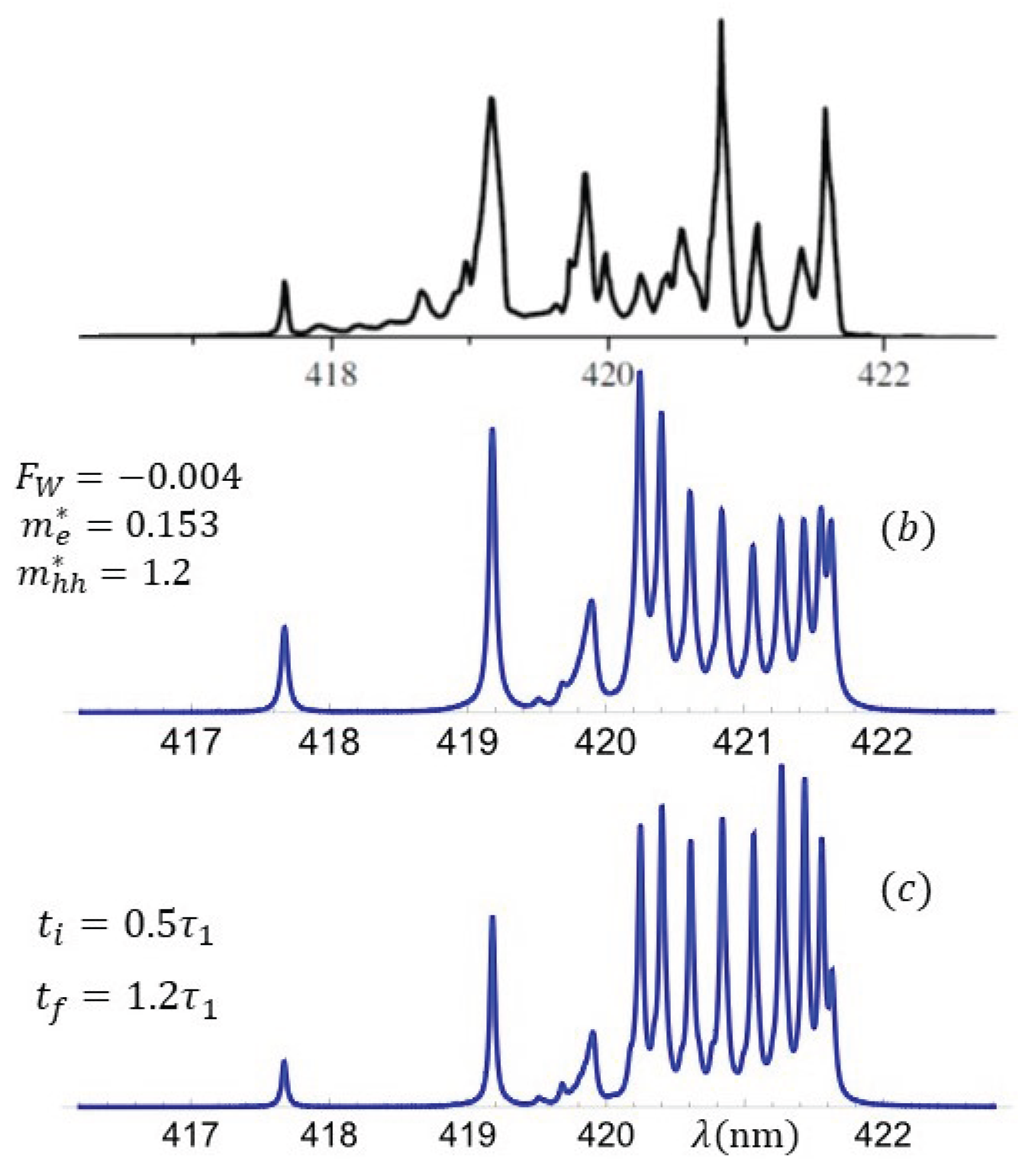
To conclude the analysis based on the time distribution of the transition probability, we summarize in Figure 11 the experimental, theoretical without time factor and the optical response evaluated with the optical susceptibility
Figure 11 shows the experimental and the theoretical spectra with and without the time factor. In the upper panel the experimental response. In panel (b) the same spectrum as in panel (b) of Figure 6, and in panel (c) the optical spectrum of Equation (45), which takes into account the polarization, symmetry and time effects. The combined effects of asymmetry, polarization, effective mass, and recombination lifetimes provide a faithful description of the blue laser diode optical response.
4. Discussion
The results presented demonstrate that including polarization fields, asymmetry of the confining layers, and recombination lifetimes leads to a faithful reproduction of Nakamura’s blue laser spectra. Importantly, the analysis shows that effective masses in quasi-two-dimensional superlattices are significantly smaller than commonly reported bulk values. This reduction in effective mass, while not the central motivation of this work, emerges naturally from the requirement to reproduce experimental data.
The role of polarization is primarily as a fine-tuning mechanism: it shifts energy levels slightly and redistributes level spacing, consistent with Stark-effect tendencies, but does not strongly alter the overall spectrum width. By contrast, asymmetry in the confining layers has a pronounced effect on surface states, broadening the spectral features and modifying peak positions. Finally, incorporating recombination lifetimes provides a more realistic description of peak intensities and spectral evolution. Together, these results underscore the importance of including both structural asymmetry and dynamical effects when modeling superlattice-based optoelectronic devices.
5. Conclusions
We have developed and applied an exact quantum theory for polarized and asymmetric superlattices, incorporating piezoelectric polarization, confining-layer asymmetry, and recombination lifetimes. This approach, based on analytical solutions of the Schrödinger equation within the Theory of Finite Periodic Systems, allows precise calculation of eigenvalues, eigenfunctions, and optical spectra.
The theory reproduces Nakamura’s blue laser spectra with high fidelity. The analysis demonstrates that realistic reproduction requires adopting smaller effective masses than typically assumed for bulk materials, unless unphysical barrier parameters are used. While polarization primarily plays the role of a fine adjustment, asymmetry significantly affects spectral width and surface-state contributions. Moreover, recombination lifetimes, when treated through their time-dependent distribution, account for the energy dependence of peak intensities and spectral evolution.
These findings not only clarify the role of polarization and asymmetry in superlattice devices but also highlight the need to revisit effective-mass assumptions in quasi-two-dimensional systems. The methodology and insights provided here may guide the design and optimization of next-generation optoelectronic devices.
Author Contributions
Conceptualization, P.P.; methodology, P.P.; software, V.I-S. and P.P.; investigation, P.P. and V.I-S.; original draft preparation, P.P.; review and editing, P.P. and V.I-S. All authors have read and agreed to the published version of the manuscript.
Data Availability Statement
The data presented in this study are available on request from the corresponding author due to legal restrictions.
Acknowledgments
The authors are members of the Sistema Nacional de Investigadoras e Investigadores (SCHTI, Mexico) and acknowledge its economical support.
Conflicts of Interest
The authors declare no conflicts of interest.
References
- S. Nakamura, M. Senoh, S. Nagahama, N. Iwasa, T. Yamada, T. Matsushita, H. Kiyoku and Y. Sugimoto, Appl. Phys. Lett. 68, 3269 (1996); S. Nakamura, T. Mukai, Japan. J. Appl. Phys. 31, L1457 (1992). [CrossRef]
- S. Nakamura, S. Pearton, G. Fasol, The Blue Laser Diode. The complete history (Springer-Verlag, Berlin Heidelberg 1997). See page 247 of.
- A. Usui, H. Sunakawa, A. Sakai, A. Yamagushi, Japan. J. Appl. Phys. 36, L899 (1997). [CrossRef]
- O.H. Nam, M.D. Bremser, T. Zheleva, R.F. Davis, Appl. Phys. Lett. 71, 2638 (1997). [CrossRef]
- L. Bergman, M. Dutta, M.A. Strocio, S.M. Komirenko, R.J. Nemanich, C.J. Eiting, D.J.H. Lambert, H.K. Kwon, R.D. Dupuis, Appl. Phys. Lett. 76, 1969 (2000). [CrossRef]
- T. Mukai, S. Nagahama, M. Sano, T. Yanamoto, D. Morita, T. Mitani, Y. Narukawa, S. Yamamoto, I. Niki, M. Yamada, S. Sonobe, S. Shioji, K. Deguchi, T. Naitou, H. Tamaki, Y. Murazaki, M. Kameshima, Phys. Status Solidi a 200, 52 (2003). [CrossRef]
- I.I. Reshina, S.V. Ivanov, D.N. Mirlin, I.V. Sedova, S.V. Sorokin, Semiconductors 39, 432 (2005). [CrossRef]
- Y. Sun, Y. H. Cho, E. K. Suh, H. J. Lee, R. J. Choi, and Y. B. Hahn, Appl. Phys. Lett. 84, 49 (2004).
- A. Kikuchi, M. Kawai, M. Tada, and K. Kishino, Jpn. J. Appl. Phys., Part 2 43, L1524 (2004). [CrossRef]
- R. Ascazubi, I. Wilke, K. Denniston, H. Lu, and W. J. Schaff, Appl. Phys. Lett. 84, 4810 (2004).
- P. Schley, R. Goldhahn, C. Napierala, G. Gobsch, J. Schoermann, D. J. As, K. Lischka, M. Feneberg, and K. Thonke, Semicond. Sci. Technol. 23, 055001 (2008).
- T. Matsuoka, Superlatt. Microstruct. 37, 19 (2005).
- J. Wu J. Appl. Phys. 106, 011101 (2009).
- M. L. Badgutdinov, and A. E. Yunovich, Semiconductors 42, 429 (2008).
- M. Jarema, M. Gładysiewicz, Ł. Janicki, E. Zdanowicz, H. Turski, G. Muzioł, C. Skierbiszewski, and R. Kudrawiec, J. App. Phys. 126, 115703 (2019).
- P. Pereyra, Phys. Rev. Lett. 80 2677 (1998); P. Pereyra, J. Phys. A Math. Gen. 31, 4521 (1998). P. Pereyra and E. Castillo, Phys Rev. B 65, 205120 (2002).
- P. Pereyra, Ann. Phys. 320, 1 (2005).
- A. Anzaldo-Meneses and P. Pereyra, Ann. Phys. 322, 2114 2007.
- P. Pereyra, Ann. Phys. 378, 264 (2017).
- P. Pereyra, Phys. Status Solidi B 259, 2100405 (2022).
- F. Assaoui and P. Pereyra, J. Appl. Phys. 91, 5163 (2002). [CrossRef]
- A. Kunold, P. Pereyra, J. Appl. Phys. 93, 5018 (2003). [CrossRef]
- M. Fernanda Avila-Ortega and P. Pereyra, Superlatt. and Microstruct. 43, 645 (2008).
- P. Pereyra, Ann. Phys. 397, 159 (2018).
- F. Bernardini, V. Fiorentini and D. Vanderbilt, Phys. Rev. B 56, R10024 (1997). [CrossRef]
- P. Kozodoy, Monica Hansen, S. P. Denbaars and U. K. Mishra, Appl. Phys. Lett. 74, 3681 (1999). [CrossRef]
- S. Hackenbuchner, J. A. Majewski, G. Zandler, G. Vogl, J. Crystal. Growth. 230, 607 (2001). [CrossRef]
- D. Goepfert, E. F. Schuber, A. Osinsky, P. E. Norris and N. N .Faleev, Appl. Phys. Lett. 88, 2030 (2000).
- P. Perlin, S. P. Lepkowski, H. Teisseyre, T. Suski N. Grandjean and J. Massies, Acta. Physica. Polinica A. 100, 261 (2001). [CrossRef]
- N. Grandjean, J. Massiers, S. Dalmasso, P. Vennegues, L. Siozade and L. Hirsch, Appl. Phys. Lett. 74, 3616 (1999).
- R. Langer, A. Barski, J. Simon, N. T. Pelekanos, O. Konovalov, R. Andre and Le Si Dang, Appl. Phys. Lett. 74, 3610 (1999). [CrossRef]
- P. Pereyra and F. Assaoui, J. Nanophotonics 11, 020501-1(2017).
- M. Anikeeva, M. Albrecht, F. Mahler, J. W. Tomm, L. Lymperakis, C. Chèze, R. Calarco, J. Neugebauer, and T. Schulz Scientific Reports 9, 9047 (2019). [CrossRef]
- P. Pereyra, J. Optics 26, 075501 (2024).
- M. Pacheco, F. Claro Phys. Stat. Sol. b 114, 399 (1982); B. Ricco, M.Ya. Azbel, Phys. Rev. B 29 , 1970 (1984); R. Pérez-Alvarez and H. Rodriguez-Coppola, Phys. Status Solidi (b) 145, 493 (1988); T. H. Kalotas, A. R. Lee, Eur. J. Phys. 12, 275 (1991); D. J. Griffiths, N. F. Taussing, Am. J. Phys. 60, 883 (1992); D. W. Sprung, H. Wu, J. Martorell, Am. J. Phys. 61, 1118 (1993); M. G. Rozman, P. Reineker, R. Tehver, Phys. Lett. A 187, 127 (1994).
- R. C. Jones, J. Opt. Soc. Am 31, 500 (1941).
- F. Abelès, Ann. Phys. 3, 504 (1948),.
- P. Pereyra, J. Math. Phys. 36, 1166 (1995).
- J. Wu, W. Walukiewicz, Semicond. Superlatt. 34, 63 (2003).
- H. Althib Crystals 12, 1166 (2022). [CrossRef]
- N. Armakavicius, S. Knight, Ph. Kühne, V. Stanishev, D.Q. Tran, S. Richter, A. Papamichail, M. Stokey, P. Sorensen, U. Kilic, M. Schubert, P.P. Paskov, and V. Darakchieva APL Mater. 12, 021114 (2024). [CrossRef]
- S. Berrah, A. Boukortt, and H. Abid Semicond. Phys. Quant. Electr. & Optoelectr.,11, 59 (2008).
- A. Said, Y. Oussaifi, N. Bouarissa and M. Said Int J Opt Photonic Eng 6, 35 (2021). [CrossRef]
- V.Y. Davydov, A.A. Klochikhin, V.V. Emtsev, D.A. Kurdyukov, S.V. Ivanov, V.A. Vekshin, F. Bechstedt, J. Furthmüller, J. Aderhold, J. Graul, A.V. Mudryi, H. Harima, A. Hashimoto, A. Yamamoto, and E.E. Haller Phys. Stat. Sol. (b) 234, 787 (2002).
- Z. Dridi, B Bouhafs and P Ruterana Semicond. Sci. Technol. 18, 850 (2003). [CrossRef]
- D. Pashnev, V.V. Korotyeyev, J. Jorudas, T. Kaplas, V. Janonis, A. Urbanowicz, and I. Kašalynas Appl. Phys. Lett. 117, 162101 (2020). [CrossRef]
- P. Pereyra Europhys. Lett. 125, 27003 (2019). [CrossRef]
| 1 | |
| 2 | Sometimes referred to as cladding or light-guiding layers in Nakamura’s terminology [2]. |
Figure 1.
Narrow peaks and subband groups in the optical spectra observed by Nakamura et al. [1,2] (upper panel) and calculated [24] (lower panel) for the blue-emitting superlattice with , nm, and nm.
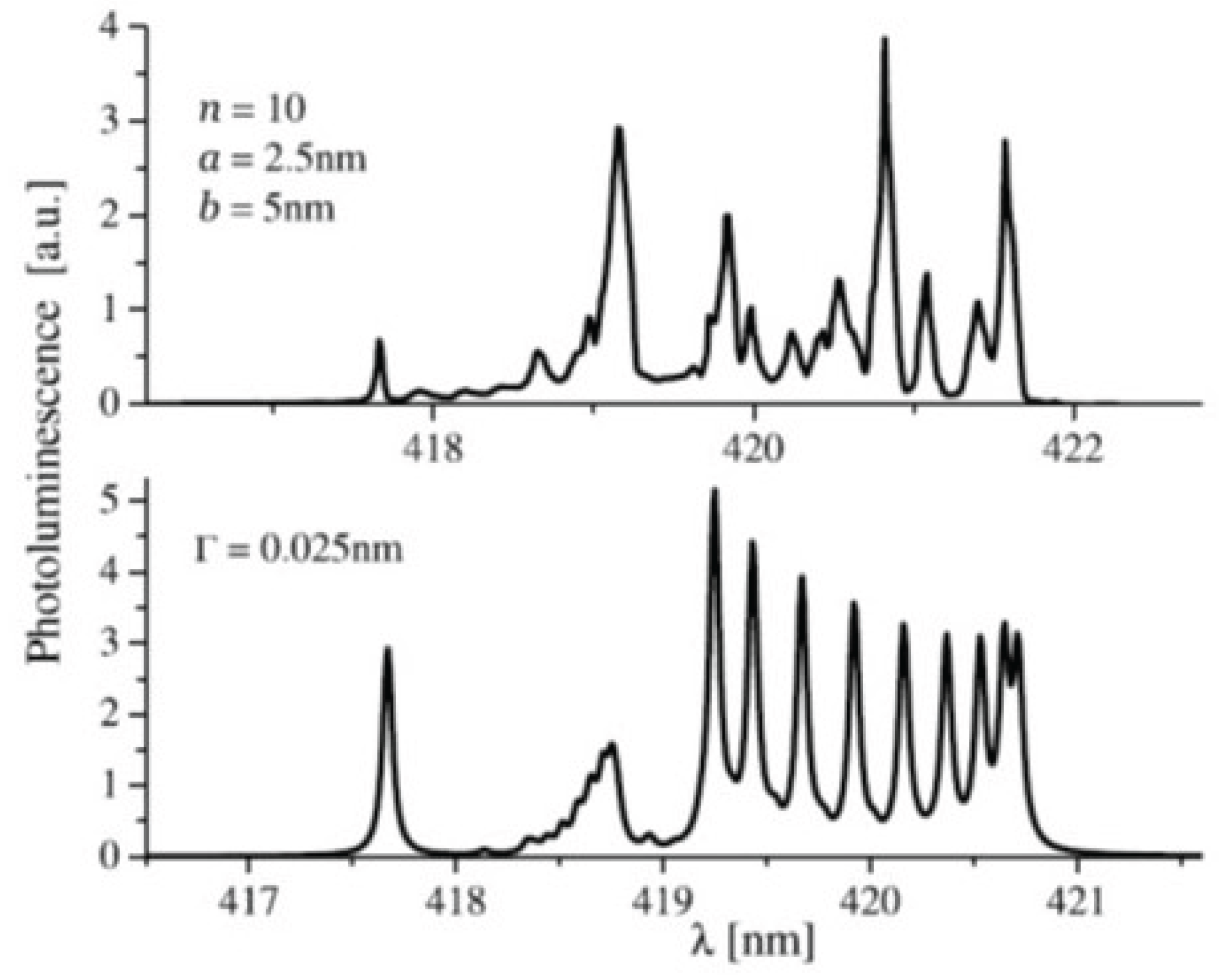
Figure 2.
Potential parameters in a biased superlattice, with and .
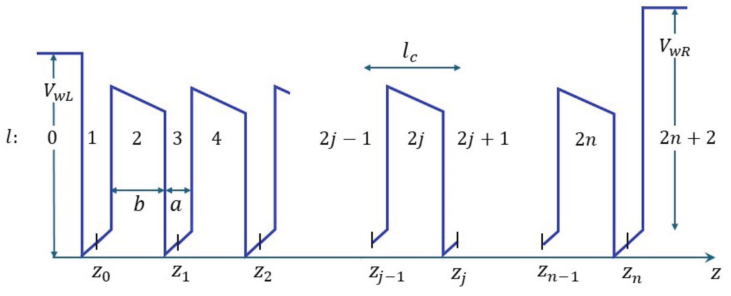
Figure 3.
Eigenfunctions and eigenvalues without and with polarization. The dominant effect of local fields is the upward shift of the energy eigenvalues.
Figure 3.
Eigenfunctions and eigenvalues without and with polarization. The dominant effect of local fields is the upward shift of the energy eigenvalues.
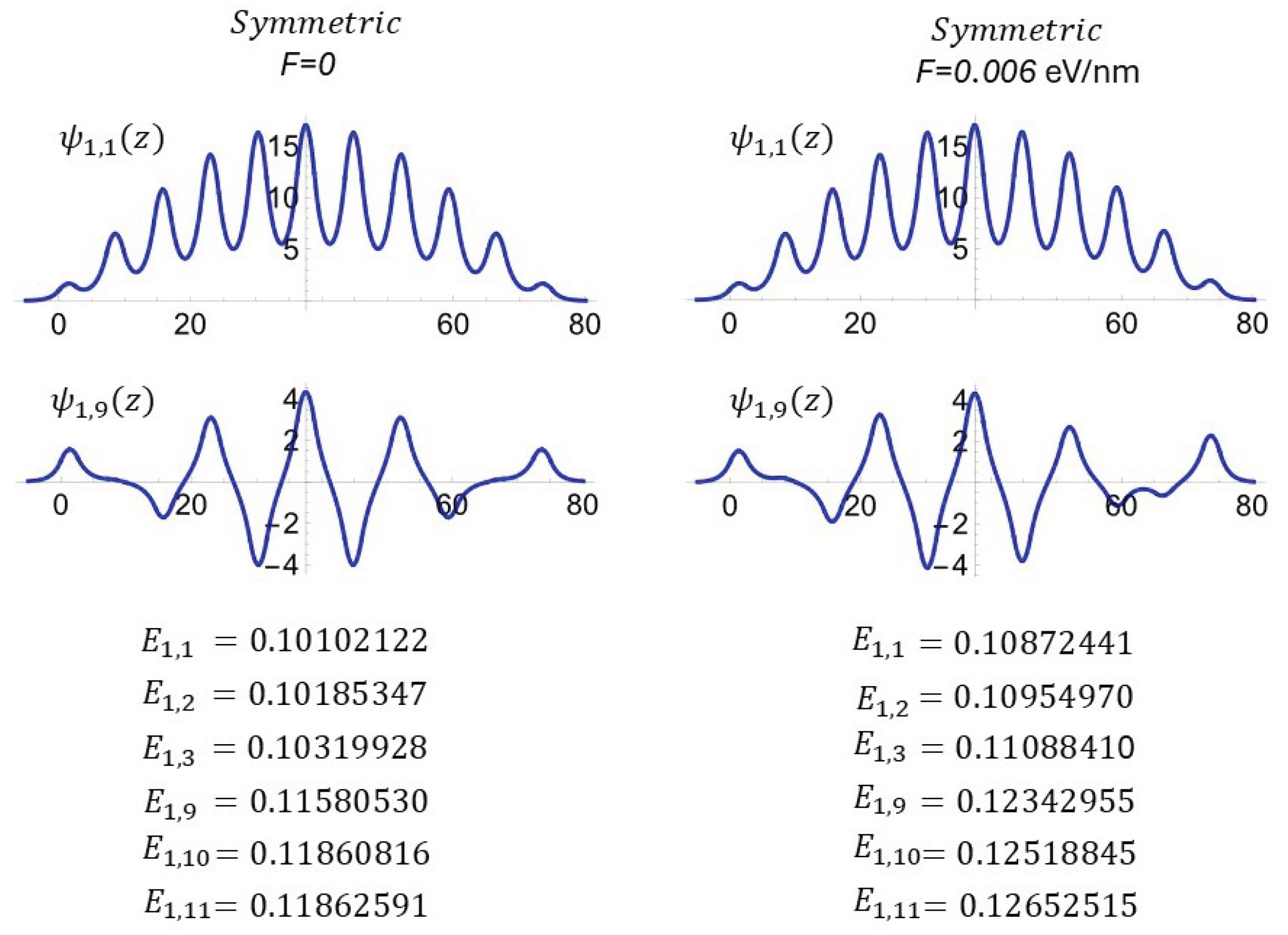
Figure 4.
Effect of confining-layer asymmetry. The asymmetry alters the symmetry of the eigenfunctions and shifts one of the surface-state energy levels further away.
Figure 4.
Effect of confining-layer asymmetry. The asymmetry alters the symmetry of the eigenfunctions and shifts one of the surface-state energy levels further away.
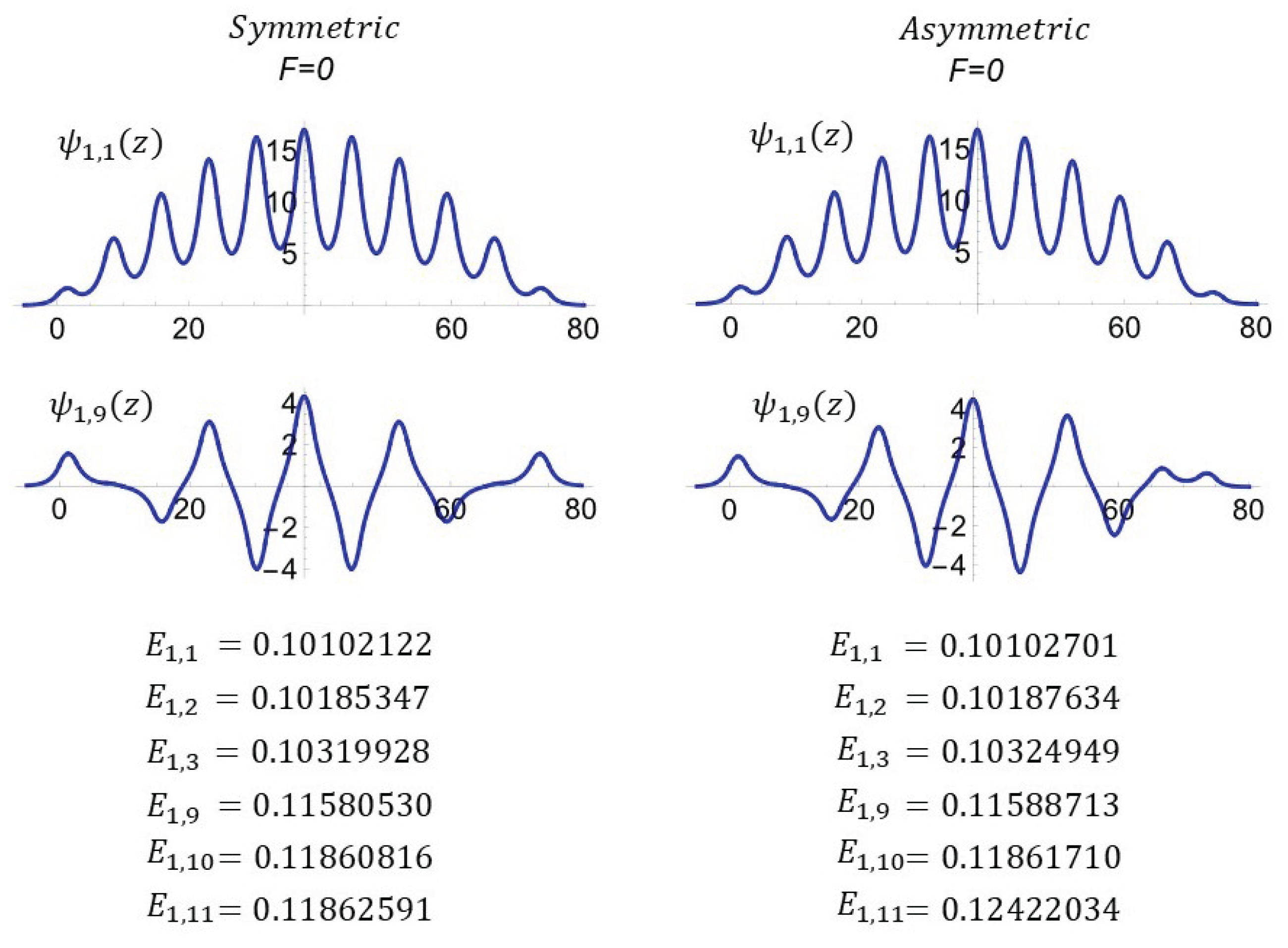
Figure 5.
Subband width as a function of the effective mass. To reproduce the experimental spectrum width (blue bar), the effective mass should be of the order of 0.15.
Figure 5.
Subband width as a function of the effective mass. To reproduce the experimental spectrum width (blue bar), the effective mass should be of the order of 0.15.
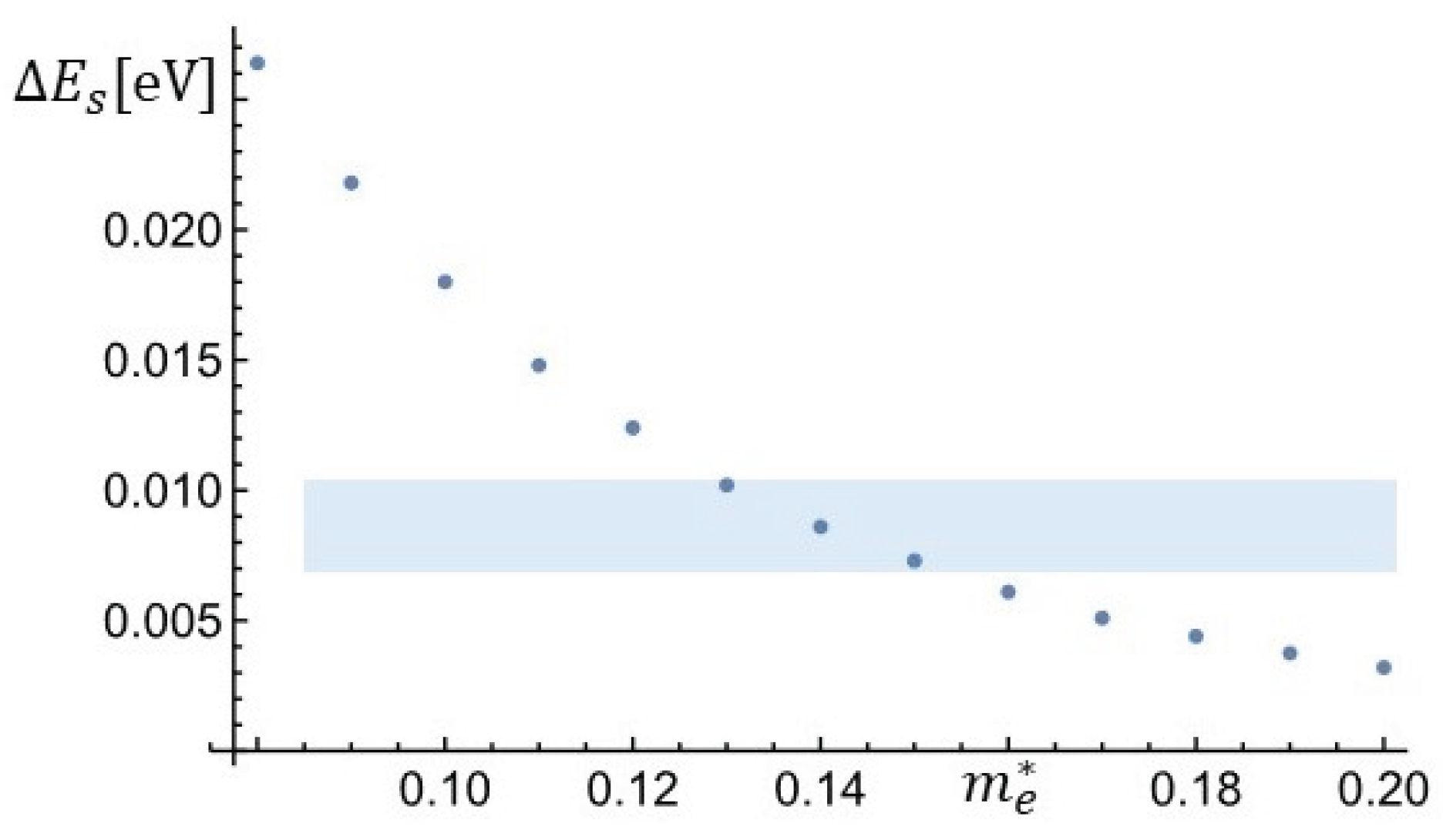
Figure 6.
Experimental result and theoretical spectra for two sets of parameters. In the left-hand column we show the best fits obtained for barrier height eV, with negative (b) and positive (c) polarization fields, and lateral potential heights .27 eV and .36 eV. In the right-hand column we show the best fits obtained for barrier height eV, with negative (d) and positive (e) polarization fields, and lateral potential heights .285 eV and .381 eV. The corresponding effective masses are indicated in the panels, and the asymmetries in the text.
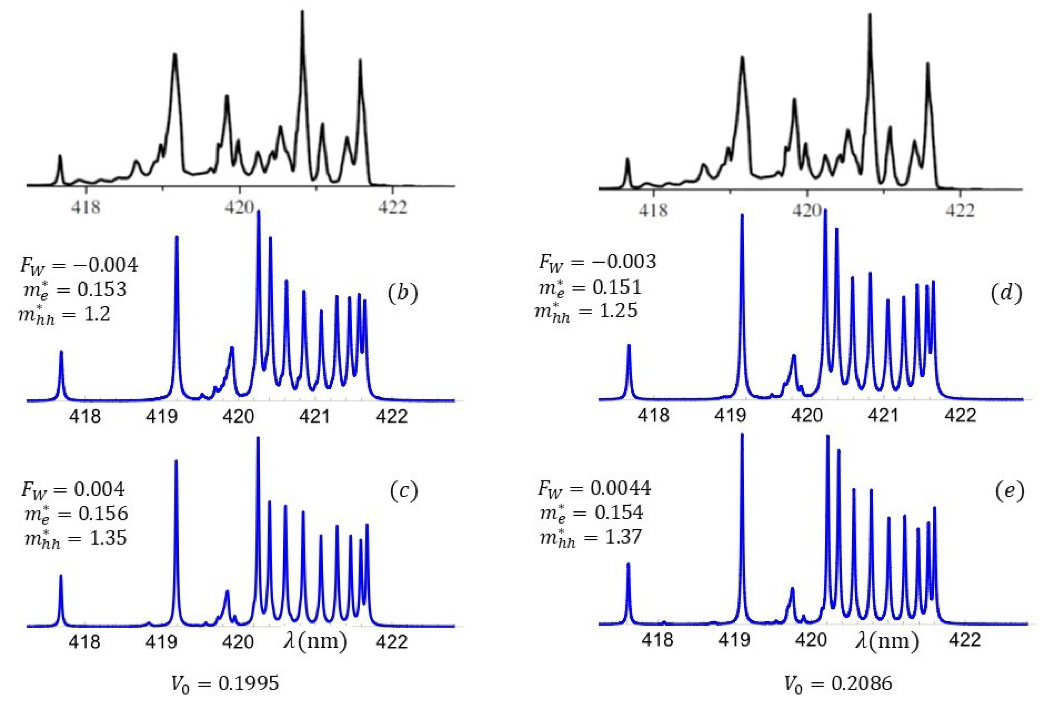
Figure 7.
Asymmetry and local-field effects on the optical response spectrum of a SL. Left column: effect of asymmetry of the confining potential, with polarization field and effective masses fixed at eV/nm, , and . Increasing the confining asymmetry from (practically symmetric, slightly broken by the Stark effect) to the reported asymmetry in Nakamura’s sample, we see not only the relation between asymmetry and the isolated peak, but also how the repulsion of surface states affects the spectrum width. Right column: effect of the polarization field, with other parameters fixed. The field mainly shifts the spectrum, with small changes in level spacings.
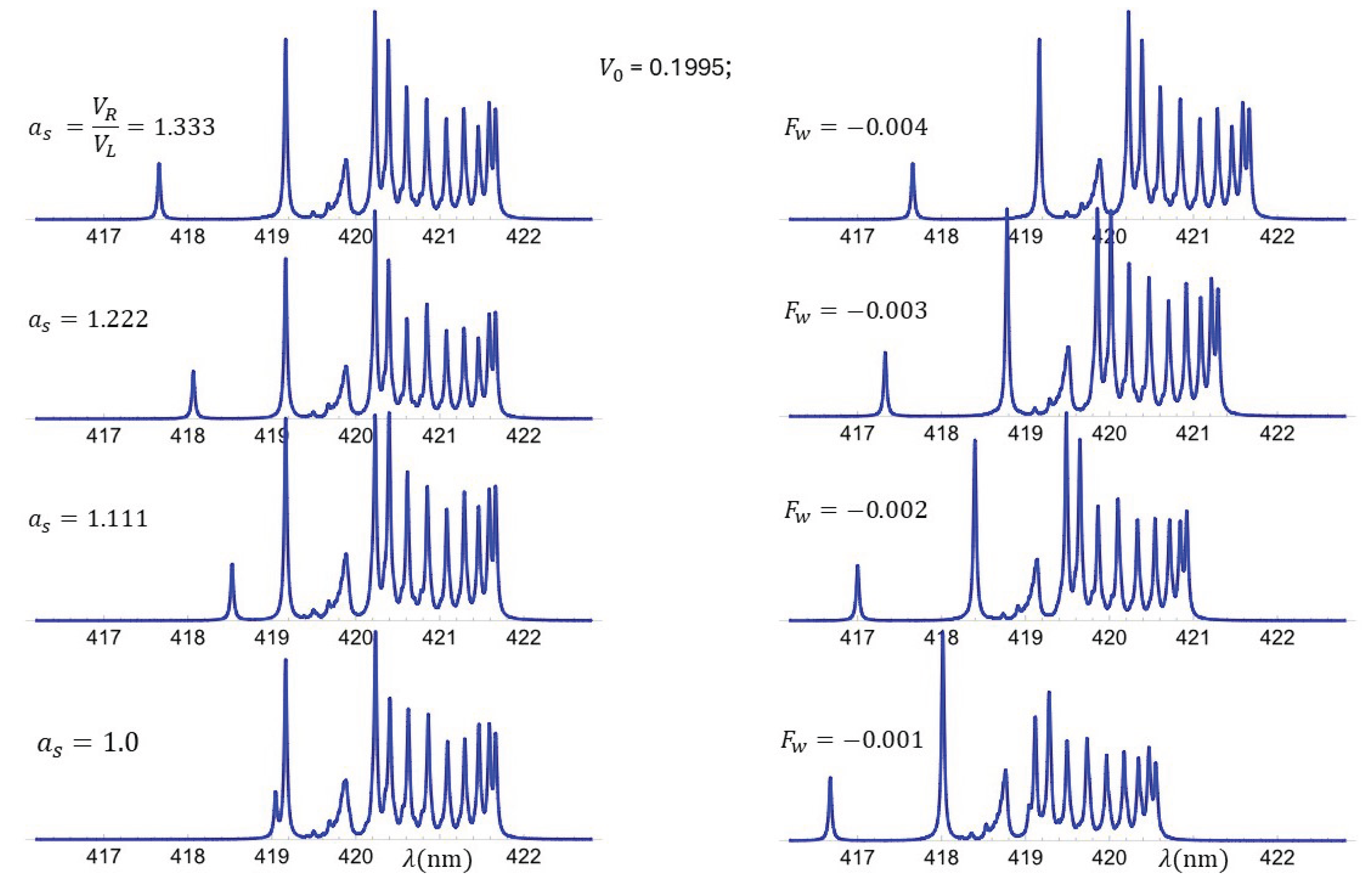
Figure 8.
Effect of effective masses on the optical spectra. Left column: electron effective mass in the superlattice wells varied from to . Increasing reduces the width of the low-energy resonance group, showing that the quasi-two-dimensional effective mass is much smaller than the bulk value. Right column: hole effective mass variation. Increasing reduces the width of the higher-energy resonance group.
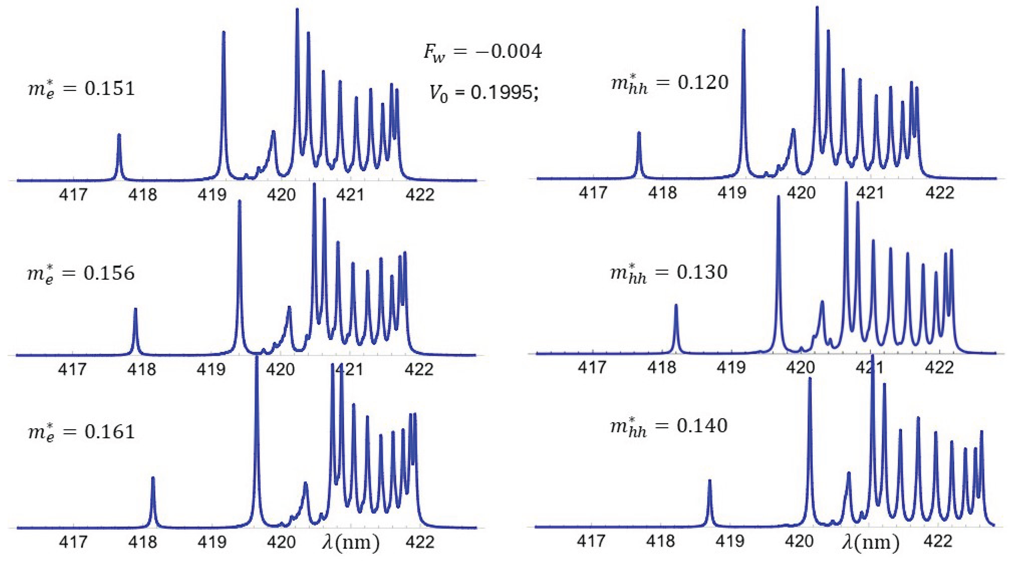
Figure 9.
Transition probability and energy-level decay contributions to the optical response. Left: time distribution of transition probability for levels , , and with decay times ns, , and . Different lifetimes lead to complex recombination dynamics, even neglecting intra-subband transitions. On the right hand side column the optical responses at two observation times . In the upper panel, at 5 ns, the time is small enough as to see the high-energy levels contributions. In the lower panel, at ns, the high energy levels resonances practically disappear and the main contributions come from the low energy level transitions.
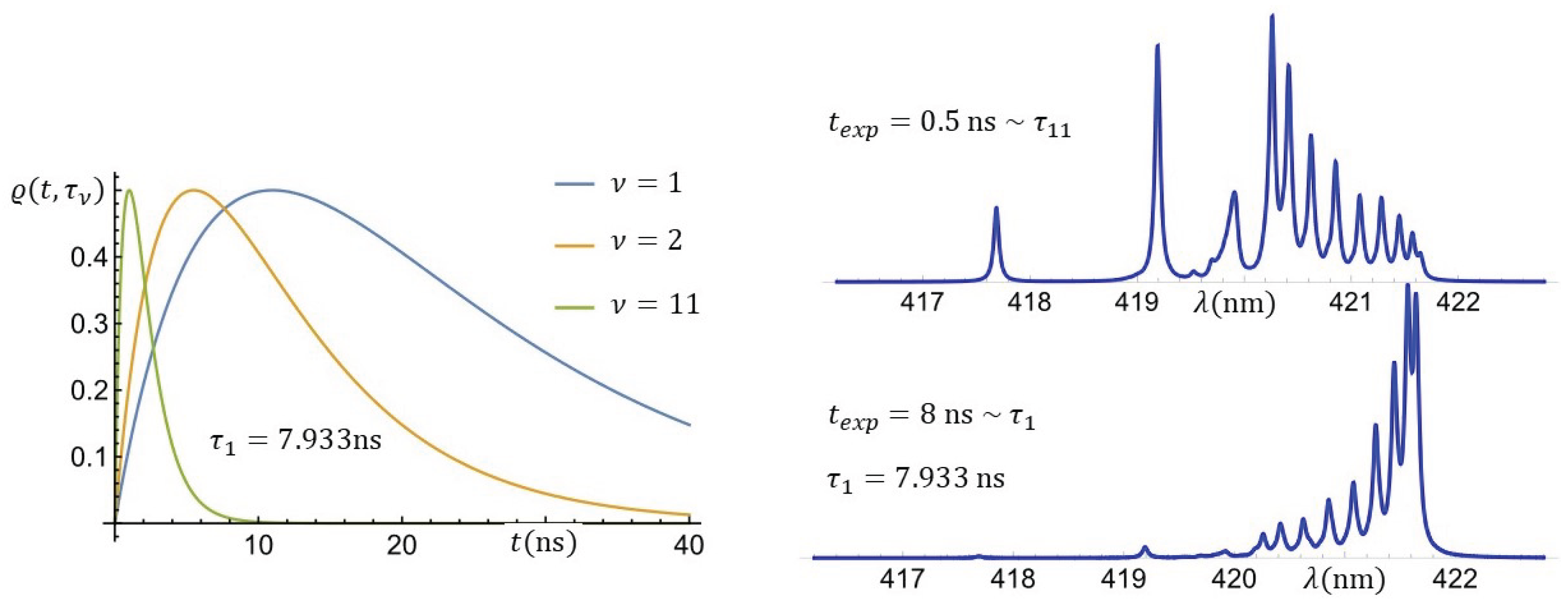
Figure 10.
Energy levels contribution and optical spectrum from data collected between and . In the left the accumulated probability as function of the energy level index for the same and different . In the right hand side column the optical spectra for two time windows of data collection. In the upper and lower panels is the same but is different.
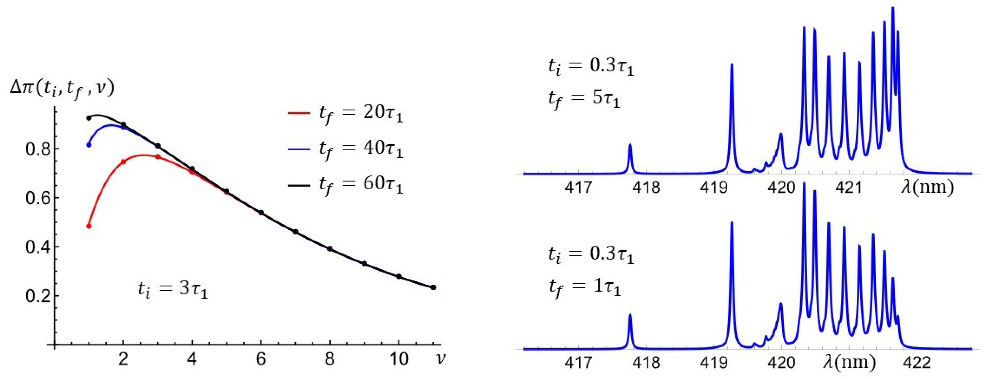
Figure 11.
The experimental and theoretical spectra. In the upper panel the experimental optical response. In panel (b) the theoretical spectrum that was shown in panel (b) of Figure 6. In panel (c) the spectra for the same set of parameters, but taking into account the time distribution of transition probabilities and a window of time between and , for data collection.
Disclaimer/Publisher’s Note: The statements, opinions and data contained in all publications are solely those of the individual author(s) and contributor(s) and not of MDPI and/or the editor(s). MDPI and/or the editor(s) disclaim responsibility for any injury to people or property resulting from any ideas, methods, instructions or products referred to in the content. |
© 2025 by the authors. Licensee MDPI, Basel, Switzerland. This article is an open access article distributed under the terms and conditions of the Creative Commons Attribution (CC BY) license (http://creativecommons.org/licenses/by/4.0/).
Copyright: This open access article is published under a Creative Commons CC BY 4.0 license, which permit the free download, distribution, and reuse, provided that the author and preprint are cited in any reuse.


