
Submitted:
17 October 2024
Posted:
18 October 2024
You are already at the latest version
Abstract
Drilling and blasting is the conventional method used for rock fragmentation in open pit mining. Blast-induced damage can reduce the level of stability of benches and pit slopes. To develop an optimal blast design, an adequate knowledge of the rock properties and in-situ fractures is needed. Fractures are generally the paths of least resistance for explosive energy and can affect the intensity of blast-induced damage. Discrete Fracture Networks (DFN) are 3D representations of joint systems used for estimating the distribution of in-situ fractures in a rock mass. The combined finite/discrete element method (FDEM) can be used to simulate the complex rock breakage process during a blast. The objective of this paper is to develop a methodology for assessing the influence of in-situ joints on the post-blast fracturing and the associated wall damage in 2D bench blasts scenarios. First, a simple one-blasthole scenario is analyzed with the FDEM software Irazu 2D and calibrated based on a laboratory-scale blasting experiment available from previous literature. Secondly, more complex scenarios consisting of one-blasthole models at the bench-scale were simulated. A bench blast without DFN (base case) and one with DFN, were numerically simulated. The model with DFN demonstrated that the growth path and intensity of blast-induced fractures were governed by pre-existing fractures which led to smaller wall damage area. The damage intensity for the base case scenario is about 42% higher than for the blast model with DFN included, which highlights the significance of in-situ fractures in the resulting blast damage intensity. The methodology for developing the DFN-included blasting simulation provides a more realistic modeling process for blast-induced wall damage assessment. This results in a better characterization of the blast damage zone and can lead to improved slope stability analyses.
Keywords:
Blast-induced damage
; Wall damage
; Discrete Fracture Network
; Combined finite/discrete element method
; Fracture intensity
; Bench blast
1. Introduction
The drilling and blasting method is widely used for rock fragmentation in open pit operations. One of the objectives in blast design is to break and fragment the desired rock mass with minimal damage to the blast boundary. The main blast in the open pit mine is referred to as production blast [1]. Blast design must be tailored to the specific rock domains for a desired outcome, i.e., targeted rock fragment size, muckpile shape, direction of displacement, minimizing fly rocks, or minimizing damage to final walls [1,2]. Depending on the blast design objectives, related factors will be modified, i.e., initiation sequence (timing), borehole dimensions, and blast patterns [1,3]. Insufficient knowledge of the rock properties and existing joints can cause delays and safety concerns in an open pit mine operation because it could result in inadequate rock fragmentation, potential fly rocks and/or wall damage. Wall damage is the extra cracking beyond the intended area of fragmentation, and this can result in instabilities and hazardous environment. This could lead to loss of production, slope failures, damage to equipment, staff injuries, and increased production time [4,5,6].
Despite the widespread use of explosives, there is a gap in understanding how to achieve specific blast outcomes. Blasting engineers often rely on empirical rules [2,7] and multiple iterations of blast designs are frequently needed to achieve optimal results. Predicting blast outcomes, such as blast-induced damage, is challenging due to the complexity of the blasting process [8]. Additionally, energy from explosive is often wasted through ground vibrations, flyrocks, etc., reducing the energy available for rock fragmentation [6]. Rock fragmentation by blasting involves wave propagation, fracture mechanics principles, large material displacement, and interactions among these processes [8]. The presence of natural fractures in the rock mass and their influence on explosive waves attenuation are significant factors in achieving the desired blast outcome [9]. A good understanding of structural features (e.g., in-situ fractures networks) and reliable numerical simulations of the blasting process can aid in overcoming these challenges. Since the blasting process starts with stress waves propagation and proceeds to a large material displacement, effective modeling should incorporate both continuum and discontinuum models to represent the process more reliably [10].
1.1. Mechanism of Rock Breakage by Blasting
Rock blasting is a complex dynamic process with multiple mechanisms involved. Upon detonation, the explosive generates a shock wave that pulverizes the rock near the blasthole. Following this, compressive stress waves propagate radially from the blasthole. The compressive waves first create microfractures around the blasthole which promotes additional rock fracturing. When they reach open surfaces, stress waves then reflect off this free face (e.g., bench face), transforming to tensile stress waves that further develop and expand fractures. The chemical reaction of the explosive produces high gas pressure, which further contribute to fracture propagation and rock fragmentation, resulting in the formation of a muckpile [3,11].
1.2. Discrete Fracture Network (DFN)
In a rock mass, the intersection of natural joints (or fractures) form in-situ blocks. The existence of these geological features causes challenges in designing bench-scale blasts [11,12]. The natural joints are considered the main points for blast-induced damage to develop [13]. Fragmentation of rock by blasting is the result of the coalescing of pre-existing and blast-induced fractures in the rock mass. Discrete Fracture Networks (DFN) are 3D representations of joint systems that can estimate the distribution of in-situ fractures and block sizes based on field measurements of the fracture properties, i.e., fracture orientation (dip and dip direction) and intensity; and using statistical distributions.
The DFN community developed a unified system, the Pij system (Table 1), to characterize fracture intensity. The Pij system offers a straightforward approach in terms of scales and dimensions: the indices i and j stand for dimension of sample and dimension of measurement, respectively [14]. Of the available fracture intensity measures, P32 (fracture area per unit volume) is the preferred measure for DFN modelling since this represents a non-directional intrinsic measure of fracture intensity [15]. Whilst P32 cannot be directly measured, it can be estimated from either P10 or P21 measurements [15,16].
A DFN-based analysis relies on quantifiable joints properties and provides realistic fracture networks with the key advantage of preserving the real joint properties during the modelling process. Additionally, the DFN approach creates models in smaller scale more accurately in comparison to large-scale continuum methods [14,15], which is appropriate at the scale of production blasts.
1.3. Numerical Simulation of a Bench Blast
Over the past decades, various numerical methods were developed for simulating and solving engineering problems. Due to the fractured nature of many rock masses, the numerical simulation of the rock mass behavior could fall in either of the two categories: continuous or discontinuous approaches [18]. In rock blasting, the rock mass can be treated as a continuum before the fracturing process. Finite element method (FEM) and Finite difference method (FDM) can calculate the stress distribution and the deformation in the rock; and predict the damage or fracture pattern in a continuum [3]. For continuum mechanical problems, the FEM is widely used for simulating large domains or fracture propagation [19,20]. The discrete element method (DEM) is the most used method for discontinuum problems such as fluid flow in fractured medium or large displacements caused by blasting [3,19].
During rock blasting, the rock mass receives a dynamic load which fragments the rock and moves the resulting rock fragments in designated direction(s) determined by blast design. Such processes occur at different scales and with different behaviors. When the fragmented rocks are being ejected as the result of the gas expansion and blasting waves, the movement is large enough that could not be modeled with continuum approaches [3]. FEM-only or DEM-only approaches are not adequate for simulating rock fragmentation by blasting [21]. Additionally, the difference between the scale required for analyzing the fracture and damage mechanics, and the scale of the rock mass is another concern which directly relates to limitations of each numerical method if used separately [22]. The effects of the discontinuities on wave propagation are also an important interaction to be considered in blasting operations [8,9]. A fractured rock medium would have an impact on wave attenuation, and hence, a higher dynamic resistance in comparison to an intact medium [8,23,24].
The combined finite-discrete element method (FDEM) was proposed by Munjiza et al. [25] and Munjiza [26]. This is an advantageous method for simulating the deformability, discontinuity development and the transition between these processes [24]. The processes that transition from continuum to discontinuum media could be simulated using FDEM by incorporating the contact detection interface analysis, as well as fracture creation and propagation [20,24]. Zhang [3] discusses the capability of FDEM to numerically represent the blasting process. In the context of an open pit bench blast, FEM is used to model stress distributions, as well as small displacements in rock before fracture initiation. DEM is then employed to model the fractured medium, simulating fracture creation and propagation, as well as the large displacements of rock fragments that lead to muckpile formation.
In this paper, the effects of pre-existing fractures in the rock mass during an open pit bench blast were investigated by integrating a DFN model in a FDEM blasting simulation. The combination of these two numerical tools provides an opportunity to represent the bench blasting mechanism more reliably and to investigate the influence of in-situ fractures in the extent of blast-induced wall damage. The goal is to develop a methodology for quantifying the level of blast-induced wall damage by comparing two scenarios: 1. A bench blast without DFN (base case), and 2. A bench blast with DFN included. The comparison between the two scenarios highlights the difference in wall damage profile in presence of in-situ fractures. This damage assessment methodology lays the groundwork for model calibration in a future study and expansion of the developed methodology to production bench blast models with multiple rows of blastholes. Section 2 describes the pressure boundary formulations used for simulating the blasting process in Irazu 2D V5.0 [27]. This process was verified using a simple scenario considering a laboratory-scale experiment from available literature. Section 3 presents the more complex single-hole blast scenario developed at the bench-scale. The results of the bench blast simulations and assessment of the effects of pre-existing fractures on the extent of blast-induced damage are discussed in Section 4.
2. Blasting Pressure Boundary Formulations
Available literature has provided equations to calculate various blasting parameters. Hajibagherpour et al. [28] developed an equation to determine the maximum detonation pressure within a borehole (Equation (1)).
where is the detonation pressure (MPa), VOD is velocity of the detonation (m/s), ρe is explosive density (g/cm3), is explosive diameter (mm), and is blasthole diameter (mm). When the explosive is fully coupled in the blasthole (dc/dh = 1), Equation (1) could be written as Equation (2):
The peak gas pressure generate after a blast could be calculated using Equation (3) [29]:
where Pb is gas pressure (Pa), VOD is velocity of detonation (m/s), ρe is the density of explosive (Kg/m3), fc is coupling factor (ratio of the volume of the explosive to the volume of the blasthole excluding the stemming column), and n is coupling factor exponent (value between 1.2 and 1.3 for dry holes and 0.9 for holes filled with water) [29]. For a fully coupled explosive, the Equation (3) could be written as Equation (4):
A pressure-time curve is required to apply detonation and gas pressures with regards to time steps for FDEM analysis. This pressure-time curve represents the increase of pressure to maximum detonation or gas pressure and decaying over time, reaching a value of zero. Equation (5) is used for determining pressure as a time function [30,31].
where is the time history of the dynamic load imposed on blasthole boundary (Pa), P is the detonation () or gas (Pb) pressures (Pa), β is damping factor (1/s), and t is time (s). β is calculated with Equation (6) [30,32].
where is the rise time (time of peak pressure). This parameter is calculated by maximum velocity in different media and length of the media [28]. Lu et al. [33] presented Equation (7) to calculate the rise time:
where Le is the length of the column charge (m) and VOD is the velocity of detonation (m/s). Oswald [34] modified this formulation by multiplying Equation (7) by K, an empirical factor for the gas pressure rise time. Equation (8) presents the modified equation for the rise time:
The blasting pressure formulations are used to develop pressure time curves to apply detonation and gas pressure with regards to time steps for FDEM analyses.
2.1. Laboratory-Scale Simulation for the Fractured Zone Around a Blasthole
In rock blasting, the stress waves inflict high pressure on the rock mass in a short period of time. In some cases, depending on the type of explosive and blasthole dimeter, the stress wave peak pressure could surpass 10 GPa [28]. These waves pulverize the rock surrounding the blasthole, initiate damage in the rock mass, and pave the path for the explosive gas to fragment and displace the rock medium. With the recent developments in numerical FDEM modelling tools, the rock response to explosive energy can be simulated more reliably. In order to validate the developed methodology for blast damage assessment, a simple scenario is first analyzed and compared to the results of a laboratory-scale experiment conducted by Banadaki [35].
Hajibagherpour et al. [28] developed a numerical model of the blast-induced damage surrounding a blasthole, based on the laboratory experiments conducted by Banadaki [35]. The laboratory-scale experiments consisted of Barre granite core samples with a diameter of 144 mm and a height of 150 mm. Central boreholes were drilled along the length of the cores, with 9.65 mm and 6.45 mm diameter, respectively. Copper tubes were installed on the blastholes’ boundary to focus on the shock waves and remove the effect of gas pressure. The blast was induced using DYNO cords in the blasthole and air as a coupling media. The pressure generated by the stress waves was recorded at different distances from the blast source [28,35]. In this paper, the first sample with the diameter of 9.65 mm is analyzed to validate blast-damage assessment methodology developed with the FDEM software Irazu 2D version 5.0. Figure 1 presents the schematic view of the sample, and the model simulated with Irazu. Figure 2 depicts the geometry of the blasthole. The red boundary surrounding the blasthole in Figure 1b and Figure 2b is the detonation pressure boundary.
Table 2 and Table 3 present the elastic and strength properties of rock and copper tube. The selected rock mesh size is 2 mm in order to obtain a mesh ratio, i.e., a ratio of the largest element length along the wave propagation to the smallest wavelength, smaller than 1/8 to 1/10 [28].
The explosive used in the experiment is DYNO Cord with diameter of 1.70 mm, density of 1.32 g/cm3, and VOD of 6690 m/s [28,35] Using Equation (1), this results to a peak detonation pressure of 200 MPa. Figure 3 presents the detonation pressure-time curve used for FDEM analysis.
To compare the results between the simulation performed with the FDEM software Irazu (this paper), the code developed by Hajibagherpour et al. [28], and the laboratory-scale experiment conducted by Banadaki [35], the peak pressures evaluated at three the monitoring points (Figure 1a) and the number of radial cracks developed within the rock domain were compared and the results are presented in Table 4 and Table 5. The largest pressure difference between the FDEM simulation in Irazu and the pressure monitored during the laboratory experiment is observed at monitoring point 2, with a magnitude of 2.8 MPa. Figure 4a presents the fractures developed with the FDEM simulation, the results from Hajibagherpour et al. [28] (Figure 4b) and from the laboratory-scale experiment [35] (Figure 4c). The number of radial fractures obtained from the laboratory experiment and the numerical simulations are compared in Table 5. The simulation presented by Hajibagherpour et al. [28] has generated 8 radial fractures, as opposed to 9 fractures in the laboratory-scale experiment. The simulation conducted with Irazu 2D in this paper has generated 9 radial fractures. The results obtained with the FDEM software Irazu and the blasting pressure boundary formulations are in good agreement with the lab-scale experiment results. The developed methodology was then expanded to a more complex blasting simulation at the bench-scale, as presented in Section 3.
3. Single-Hole Bench-scale Blasting Scenarios
Two blasting scenarios at the bench-scale were considered for this paper and simulated in a 2D environment. Scenario 1 represents a bench blast simulation without considering the effect of the pre-existing in-situ fractures and scenario 2 includes a network of fractures in the blasting simulation. The benches are designed based on rock and blast design properties obtained from an operating open pit gold mine. This mine site uses vertical blastholes to achieve vertical benches in their hard rock domain. Section 3.1 describes the DFN model used to generate the in-situ fractures for the bench blast scenario with pre-existing fractures (scenario 2). Section 3.2. describes the FDEM numerical model setup for the two blasting scenarios and Section 3.3 describes the material and blast design properties used for the analyses. Finally, Section 3.4. presents the damage intensity formulation used for comparing the wall damage for the two scenarios analyzed.
3.1. Discrete Fracture Network (DFN) Model
The DFN model was generated using Fracman [37] based on the joint properties obtained from an operating mine. Table 6 presents the orientation (dip and dip direction) of the three joint sets present in the rock domain used for the blasting simulation. Using Dips [38], the mean orientation for each joint set, and Fisher’s K were obtained.
The P32 value used to generate the DFN model was inferred from the P21 value (length of fractures per unit area). The P21 value (0.87 m/m2) was estimated based on the joint spacing (1/frequency) reported in the mine database and assuming persistent joints over a selected bench face area. The method for inferring P32 is detailed by Elmo et al. [16]. P32 (m2/m3) can be inferred from either 1D or 2D data based on a linear correlation with P10 (m-1) or P21 (m/m2). An initial assumption is made for P32 and the resulting DFN model is sampled to establish the corresponding P10 or P21. This process is repeated to obtain a linear relation between P32 and P10 or P21 and the field P32 is established from this linear relation, using the field P10 or P21. Figure 5 presents the field P32 value inferred from P21. The field P32 and the Fisher’s constant K, representing the dispersion of the orientation cluster, are presented in Table 6.
The dimensions of the DFN model are 52 m long (X axis) × 22 m wide (Y axis) × 20 m deep (Z axis). The length and width of the model are representative of the bench scale and were set to fit the blasting simulation model. The generated 3D DFN model is presented in Figure 6a. Because the blasting scenarios are simulated in a 2D environment, a 2D longitudinal section of the 3D DFN model (Figure 6b) is defined and exported as DFN input for scenario 2. This trace plane was applied to the DFN model at distance of 10 m in the Z axis direction.
The orientations of DFN generated fractures were verified against input orientation data using DIPS [38] (Figure 7). Table 7 presents the comparison of orientation data obtained from DIPS. The variation between the input orientation and the orientation of the DFN generated fractures is generally less than 7%. The higher variation observed for J3 dip direction (13.54%) is due to its sub-horizontal orientation resulting in high variation for the dip direction value. The fracture survey error reported in the joint properties database available at the mine site is +/- 10 degrees.
3.2. Numerical FDEM Bench Blast Model
The numerical bench blast simulation was performed with Irazu 2D V5.0 [27] and consists of a single blasthole. A single blasthole analysis provides the opportunity to investigate the impact of including a DFN on blast-induced fracture development, without the influence of other blastholes. In addition, the 2D simulations offer a time-efficient approach for bench blast analysis. Figure 8 and Figure 9 present the bench geometry for the two blasting scenarios simulated. The coordinates of starting and ending point of each trace was exported from Fracman (Figure 6b) and used to define the traces in Irazu’s model creation environment. To remove the unrealistic influence of stress waves near the model boundaries, the vertical and longitudinal lengths are exaggerated. The detonation and gas pressures were applied in the form of a pressure boundary on the blasthole walls, as shown in red in Figure 8. Constraints were introduced to remove the possibility of unrealistic displacements near the edges of simulated models. The left and right boundaries of the rock domain are free to move in the vertical (Y) direction, i.e., towards the free surface representing the top of the bench. The bottom boundary of the rock is fixed to its location. The top of the bench, bench face, and pit floor are free to move under the influence of the pressure boundary. The size of the mesh elements in the simulated models start at 10 cm near the blasthole and the elements become progressively larger in size until it reaches 1 meter close to the left side and bottom boundaries. This mesh size transition results in higher resolution in domains were stress and displacement magnitudes are high (e.g., near the blasthole’s boundary). Moreover, this reduces computation time.
3.3. Properties for FDEM simulation
The bench blast simulations require input properties such as rock properties, blast design parameters and explosive properties. These properties were obtained from the database of an open pit mine site. Table 8 presents the properties used in the FDEM analysis and representing a hard rock domain, explosive materials, and incorporated DFN model. Table 9 provides blast design properties.
The viscous damping factor was set to 1 to lower numerical oscillations [39]. The damping prevents the mechanical system be subjected to continuous driving forces [40]. When the explosive energy exceeds the strength of the elements in the model, fracturing begins. The strength of these elements is determined by Mode I fracture energy (GI) and Mode II fracture energy (GII) [39]. Mode I fracture initiation and propagation occurs when the opening of a crack element reaches the intrinsic tensile strength of the element. Mode II fracture initiation and propagation occurs when the tangential slip of a crack element reaches the intrinsic shear strength of the element. The relationship between tensile strength (ft) and Mode I fracture toughness (KIC) can be determined using Equation (9) developed by Yilmaz and Unlu [30].
Mode I fracture energy (GI) is determined by using Equation 10 [41]. Mode II fracture energy (GII) can be calculated based on GI considering the ratio of GII/GI as 10:1 [27].
where is Effective Young’s modulus (MPa) which can be derived using in plain strain mode [41]. E is the Young’s modulus (MPa) and is the Poisson’s Ratio.
The friction coefficient (fr) is the tangent of friction angle (ϕ) calculated using Equation (11) [27]:
The explosive type used in this mine is a bulk explosive denoted as Heavy ANFO (a mixture of ANFO and emulsion) which is manufactured on site. The explosive is assumed to be fully coupled in the blasthole. The fractures in the DFN model are considered broken which defines them as pure frictional discontinuity surfaces [27]. The friction coefficient for the fractures was calculated using Equation (11). The friction coefficient is the tangent of equivalent internal friction angle which was obtained from the mine’s geotechnical database.
The relationship between the horizontal and vertical stress are defined as K which is: [42]. The vertical stress was calculated by multiplying the rock density and gravity. The horizontal stress can be acquired by multiplying the K and vertical stress. For this simulation, K is 0.33, the vertical stress for 1 meter depth is 27 kPa, the horizontal stress is 9 kPa. As the depth increases, both vertical and horizontal stresses magnitudes will increase, which was applied to the simulation models.
Using Equations (2) and (4) (explosive fully coupled) and the explosives properties in Table 8, the estimated peak detonation pressure is 6.9 GPa and the peak gas pressure is 3.6 GPa. By using the Equations (5)–(8), and input parameters shown in Table 8, the detonation and gas presume-time curves, and the combined pressure curve over time can be derived as shown in Figure 10. The factors K used in Equation 8 to determine the rise time are respectively 1 and 4.5 for the detonation and gas pressure, respectively. Since the gas pressure vents during the rock fragmentation and displacement stage, pressure under 5 MPa were considered zero [43]. Both detonation and gas pressures were combined to develop the Pressure-Time Curve applied to the blasthole boundary. This means both pressures are applied in unison on the blasthole boundary. This combined pressure-time curve was developed to overcome a limitation of Irazu 2D V5.0 where the gas pressure curve cannot be applied on the fractures’ boundaries. The boundary upon which the combined pressure is applied is the same for both scenarios. Thus, the comparison between scenario 1 (bench blast without DFN) and scenario 2 (bench blast with DFN included) can help in evaluating the influence of in-situ fractures on the intensity and extent of the blast-induced damage in a rock mass.
3.4. Blast-Damage Intensity Assesssment
To assess and compare the intensity of blast-induced damage in the final wall for the two scenarios analyzed, the damage intensity index was used. Lupogo et al. [44] presented the damage intensity index (Di) defined as Equation (12).
where Yielded Area is the sum of fractured elements areas in the desired section, and Total Area is the area of the blast damage zone (red boundaries in Figure 11). The total areas considered for both scenarios are 81 m2, which includes heavily damaged, partially damaged, and lightly damaged rock mass. The yielded elements are the elements that are neighboring a fracture initiated or propagated during blasting. Fractures associated to the DFN (red straight lines) on Figure 11b and Figure 12b are excluded from the blast damage assessment. The rock fragments produced are not considered as yielded elements since the focus of this research is to determine the extent of blast-induced damage. Figure 12 present examples of the yielded elements for scenarios 1 and 2.
The mesh sizes for the Total Area for both models are the same since the damage intensity formulation is heavily affected by the mesh size. A larger mesh element adjacent to a fracture result in a larger yielded area. Thus, within the Total Area for each of the scenarios, an equivalent mesh size was generated to be able to compare the damage intensity index for both scenarios. This equivalent mesh in the blast damage zone was generated by applying mesh refinement zones to control mesh size refinement. For scenario 2, the mesh size of each DFN line was adjusted to achieve the same mesh size refinement as for Scenario 1.
4. Bench Blast Simulation Results and Damage Assessment
The bench blast simulations were done using Irazu 2D [27]. Section 4.1. and Section 4.2. present the results for Scenarios 1 and 2, respectively. Section 4.3. shows a comparison of the resulting damage intensity index for both scenarios.
4.1. Scenario 1: Bench Blast without DFN (Base Case)
The pressure-time curve for the combined detonation and gas-pressure (Figure 10) was applied as a boundary condition to the blasthole boundary. Figure 13 shows the results obtained at three different time steps during the blasting process. First, stress waves are generated by the initiation of the explosive and propagate through the rock mass. Initial fractures are developed, transversally to the blasthole. After reaching the free face (bench face), the stress waves are reflected and cause additional fracturing. Once the fractures reach the free face (Figure 13a), rocks fragments are formed and the dynamic phase starts, resulting in large displacements, as shown in Figure 13b. At this time step, venting of the explosion gases has occurred and no additional damage is observed in the final wall area. The wall damage occurs during the static phase and beginning of dynamic phase when the gas pressure is high enough to propagate fractures. Figure 13c represents the muckpile formation at the end of dynamic phase.
4.2. Scenario 2: Bench Blast with DFN
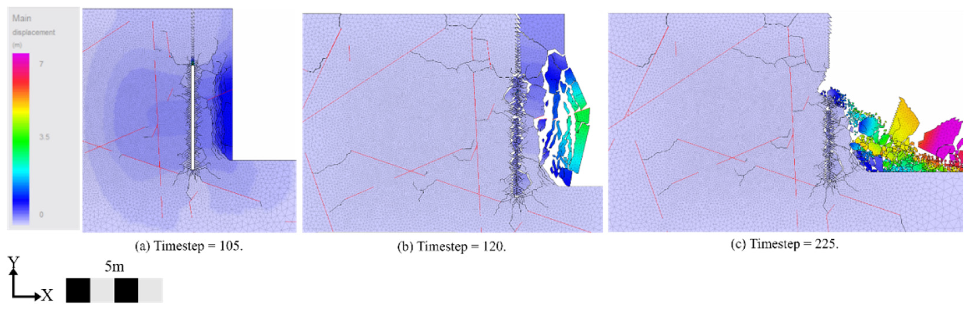
The blasting simulation for the second scenario follows the same steps as scenario 1, and it includes the DFN model presented in section 3.1, which is represented by the straight red lines in Figure 14. Figure 14 illustrates the results obtained at three different time steps during the blasting process, where the impact of the pre-existing fractures can be observed. In Figure 14a, the blast-induced fractures (in black) first propagate transversally from the blasthole and then connect to the in-situ fractures. This demonstrates that the pre-existing fractures in the rock mass influence the propagation path of the blast-induced fractures. The in-situ fractures provide paths with the least resistance for the explosive energy to dissipate. In Figure 14a, blast-induced fractures have reached the free face, rock fragments start to form an increased displacement is observed at the bench face. Figure 14b depicts the movement of the created rock fragments. When compared to scenario 1 (Figure 13b), the fragment size for scenario 2 (Figure 14b) is generally larger. This is due to the presence of in-situ fractures causing a non-uniform distribution of stress waves and allowing for some of the explosive energy to dissipate. Hence less energy is available for fragmentation, resulting in larger rock fragments. Finally, Figure 14c shows the muckpile formation.
4.3. Damage Intensity Assessment
The damage intensity for both scenarios was calculated using Equation 12. Table 10 provides the Di values for each scenario. The bench blast with DFN has a lower Di. This agrees with the results illustrated in Figure 13c and Figure 14c and demonstrates the importance of accounting for the in-situ fractures in blast-induced damage simulations. This lower damage intensity for scenario 2 is explained by the presence of in-situ fractures. The damage intensity difference is about 42 %. Effectively, explosive energy dissipates by the easiest way possible, and the presence of in-situ fractures offers paths of least resistance in the rock mass. When considering an unfractured rock mass in Scenario 1, the stress waves travel transversely through the rock medium and blast-induced fractures propagate transversely from the blasthole (Figure 13b). However, in Scenario 2, the in-situ fractures interfere with the stress waves travel path, and the propagated blast-induced fractures connect to the pre-existing fractures, resulting in only a few blast-induced fractures developed between the in-situ fractures (Figure 14b). This demonstrates well the impact of the in-situ fractures distribution on the propagation path of blast-induced fractures and on rock fragmentation.
5. Conclusion
Drilling and blasting operations aim to minimize wall damage to ensure safety for mine personnel and equipment. Numerical simulations are a valuable tool to investigate different blast design scenarios for selecting the best scenario with minimum blast-induced damage to the final rock wall. An adequate knowledge and proper representation of in-situ fracture networks are needed for assessing the level of blast-induced wall damage. The fracture network effectively influences the blast-induced fracture propagation path, the dissipation of explosive energy and gas pressure venting during the blasting process. DFN provides an opportunity for a more reliable representation of the in-situ fractures in numerical simulations of the blasting process. The combined FDEM is a capable numerical tool for simulating the static and dynamic phases of bench blasts.
Two scenarios were simulated in this paper to evaluate the impact of the in-situ fractures on the resulting wall damage: 1. A bench blast without DFN (base case), and 2. A bench blast with DFN included. The two scenarios were compared using a damage intensity index, Di. Scenario 2, which included a DFN in the numerical simulation of the blasting process, presented less blast-induced damage to the final wall (42% less damage) and larger fragment sizes in the muckpile. This demonstrated well the influence of the pre-existing fractures in the resulting blast-induced damage and fragmentation.
Finally, the results of this study demonstrated that the incorporation of a DFN model in blast-induced damage analysis can lead to a better characterization of the blast damage zone. With a more reliable blast damage assessment, improved slope stability analysis could be achieved. The presented methodology offers a reliable and computationally efficient blast-induced damage assessment in the presence of in-situ fractures. Multiple blast designs could be numerically evaluated to determine optimal blast design parameters for minimizing blast-induced damage. Given that blast design optimization is site specific, a test blast should be realized to calibrate the numerical model. However, the numerical assessment of blast-induced damage can help to reduce the number of test blasts required which results in economic benefits for the mining operation. The next step of this study is to calibrate the bench-scale blasting model with data acquired from a real blast. This will help to improve the reliability of this damage assessment methodology. After calibration, the methodology could be expanded to evaluate the extent of the blast damage zone in production bench blasts in 2D and 3D environments. Simulations in the 3D environment would help to fully capture the impact of complex 3D fracture networks.
Acknowledgments
The authors acknowledge the support of the Natural Sciences and Engineering Research Council (NSERC) of Canada (grant number RGPIN-2020-06525) and Iamgold Corporation for research funding, WSP-Golder for access to the DFN software Fracman, and Geomechanica Inc. for academic access to the FDEM software Irazu.
References
- Hall, A. Predicting Blast-Induced Damage for Open Pit Mines Using Numerical Modelling Software and Field Observations. M. A. Sc. Thesis, Laurentian University, Sudbury, ON, Canada, 2015. Available online: https://zone.biblio.laurentian.ca/handle/10219/2930.
- International Society of Explosives Engineers. ISEE blasters’ handbook, 18th ed.; ISEE: Cleveland, Ohio, 2011. [Google Scholar]
- Zhang, Z.-X. Rock Fracture and Blasting: Theory and applications; Elsevier Inc.: Cambridge, MA, USA, 2016. [Google Scholar] [CrossRef]
- Silva, J.; Worsey, T.; Lusk, B. Practical assessment of rock damage due to blasting. Int J Min Sci Tech 2019, 29, 379–385. [Google Scholar] [CrossRef]
- Kumar, S.; Mishra, AK.; Choudhary, BS. Prediction of back break in blasting using random decision trees. Eng Comp 2022, 38, 1185–1191. [Google Scholar] [CrossRef]
- Lu, Y.; Jin, C.; Wang, Q.; Han, T.; Zhang, J.; Chen, L. Numerical study on spatial distribution of blast-induced damage zone in open-pit slope. Int J Rock Mech Min Sci 2023, 163, 105328. [Google Scholar] [CrossRef]
- Dyno Nobel. Explosives Engineers’ Guide; Dyno Nobel Asia Pacific Pty Limited, 2020. Available online: https://www.dynonobel.com/apac/~/media/Files/Dyno/ResourceHub/Brochures/APAC/Explosives%20Engineers%20Guide.pdf.
- Mitelman, A.; Elmo, D. Modelling of blast-induced damage in tunnels using a hybrid finite-discrete numerical approach. J. Rock Mech. Geotech. Eng. 2014, 6(6), 565–573. [Google Scholar] [CrossRef]
- Dotto, MS.; Pourrahimian, Y. The Influence of Explosive and Rock Mass Properties on Blast Damage in a Single-Hole Blasting. Min 2024, 4, 168–188. [Google Scholar] [CrossRef]
- Han, H.; Fukuda, D.; Liu, H.; Salmi, E.; Sellers, E.; Liu, T.; Chan, A. Combined finite-discrete element modelling of rock fracture and fragmentation induced by contour blasting during tunnelling with high horizontal in-situ stress. Int J Rock Mech Min Sci 2020, 127, 104214. [Google Scholar] [CrossRef]
- Jimeno, C.L.; Jimeno, E.L.; Carcedo, F.J.A. Drilling and blasting of rocks; Taylor & Francis: New York, 1995. [Google Scholar]
- Himanshu, V. K.; Mishra, A. K.; Roy, M. P.; Shankar, R.; Priyadarshi, V.; Vishwakarma, A. K. Influence of Joint Orientation and Spacing on Induced Rock Mass Damage due to Blasting in Limestone Mines. Min Met Exp 2023, 1–11. [Google Scholar] [CrossRef]
- Zhang, P.; Bai, R.; Sun, X.; Wang, T. Investigation of Rock Joint and Fracture Influence on Delayed Blasting Performance. Appl Sci 2023, 13(18), 10275. [Google Scholar] [CrossRef]
- Elmo, D.; Rogers, S.; Stead, D.; Eberhardt, E. Discrete Fracture Network approach to characterise rock mass fragmentation and implications for geomechanical upscaling. Min Technol 2014, 123, 149–161. [Google Scholar] [CrossRef]
- Rogers, S.; Elmo, D.; Beddoes, R.; Dershowitz, W. Mine scale DFN modelling and rapid upscaling in geomechanical simulations of large open pits. In Proceedings of the International Symposium on ‘Rock Slope Stability in Open Pit Mining and Civil Engineering’, Santiago, Chile, November 2009, 11 p.
- Elmo, D.; Liu, Y.; Rogers, S. Principles of discrete fracture network modelling for geotechnical applications. In Proceedings of the First International DFNE Conference, Vancouver, British Columbia, Canada, 19-23 October 2014, 8 p.
- Dershowitz, W.; Herda, H. Interpretation of fracture spacing and intensity. In Proceedings of the 33rd U.S. Rock Mechanics Symposium, Balkema, Rotterdam, 1992, pp. 757–766.
- Elmo, D.; Stead, D.; Eberhardt, E.; Vyazmensky, A. Applications of Finite/Discrete Element Modeling to Rock Engineering Problems. Int J Geomech 2013, 13, 565–580. [Google Scholar] [CrossRef]
- Hamdi, P.; Stead, D.; Elmo, D. Damage characterization during laboratory strength testing: A 3D-finite-discrete element approach. Comp Geotech 2014, 60, 33–46. [Google Scholar] [CrossRef]
- Hazay, M.; Munjiza, A. Introduction to the Combined Finite-Discrete Element Method. In Computational Modeling of Masonry Structures Using the Discrete Element Method, Sarhosis, V., Bagi, K., Lemos, J., Milani, G., Eds.; IGI Global, 2016; pp. 123-145. [CrossRef]
- Jing, L. A review of techniques, advances and outstanding issues in numerical modelling for rock mechanics and rock engineering. Int J Rock Mech Min Sci 2003, 40, 283–353. [Google Scholar] [CrossRef]
- Wang, B.; Li, H. Contribution of detonation gas to fracturing reach in rock blasting: insights from the combined finite-discrete element method. Comput Part Mech 2024, 11, 657–673. [Google Scholar] [CrossRef]
- Jiang, X.; Xue, Y.; Kong, F.; Gong, H.; Fu, Y.; Zhang, W. Dynamic responses and damage mechanism of rock with discontinuity subjected to confining stresses and blasting loads. Int J Impact Eng 2023, 172, 104404. [Google Scholar] [CrossRef]
- Sun, G.; Sui, T.; Korsunsky, A. Review of the hybrid finite-discrete element method (FDEM). In Proceedings of the World Congress on Engineering, London, U.K., 29 June–1 July 2016, 5 p.
- Munjiza, A.; Owen, D.R.J.; Bicanic, N. A combined finite-discrete element method in transient dynamics of fracturing solids. Eng Comput 1995, 12, 145–174. [Google Scholar] [CrossRef]
- Munjiza, A. The combined finite-discrete element method, John Wiley & Sons Ltd.: Chichester, UK., 2004. [CrossRef]
- Geomechanica Inc. Irazu 2D Geomechanical Simulation Software, Theory Manual; Computer Software; Geomechanica Inc.: Toronto, ON, Canada, 2019; 67 p.
- Hajibagherpour, A.; Mansouri, H.; Bahaaddini, M. Numerical modeling of the fractured zones around a blasthole. Comp Geotech 2020, 123, 103535. [Google Scholar] [CrossRef]
- Zou, D. Theory and technology of rock excavation for civil engineering; Springer: Singapore, 2017. [Google Scholar] [CrossRef]
- Yilmaz, O.; Unlu, T. Three-dimensional numerical rock damage analysis under blasting load. Tunn Undergr Space Tech 2013, 38, 266–278. [Google Scholar] [CrossRef]
- Jong, Y.; Lee, C.; Jeon, S.; Cho, YD.; Shim, DS. Numerical modeling of the circular-cut using particle flow code In 31st Annular Conference of Explosives and Blasting Technique, Orlando, USA, 2005.
- Ainalis, D.; Kaufmann, O.; Tshibangu, JP.; Verlinden, O.; Kouroussis, G. Modelling the Source of Blasting for the Numerical Simulation of Blast-Induced Ground Vibrations: A Review. Rock Mech Rock Eng 2017, 50, 171–193. [Google Scholar] [CrossRef]
- Lu, W.; Yang, J.; Yan, P.; Chen, M.; Zhou, C.; Luo, Y.; Jin, L. Dynamic response of rock mass induced by the transient release of in-situ stress. Int J of Rock Mech Min Sci 2012, 53, 129–141. [Google Scholar] [CrossRef]
- Oswald, C. An Improved Method to Calculate the Gas Pressure History from Partially Confined Detonations. In International Explosives Safety Symposium & Exposition, San Diego, California, USA, 2018, 18 p.
- Banadaki, MMD. Stress-wave induced Fracture in Rock due to Explosive Action. Doctoral Thesis, University of Toronto, Canada, 2010.
- Wang, J.; Yin, Y.; Esmaieli, K. Numerical simulations of rock blasting damage based on laboratory-scale experiments. J Geophys Eng 2018, 15, 2399–2417. [Google Scholar] [CrossRef]
- WSP-Golder Associates. FracMan: DFN software suite; Computer software; Golder Associates: Toronto, ON, Canada, 2020; Available online: http://www.golder.com/fracman/.
- Rocscience Inc. DIPS Tutorial (version 8); Computer Software; Rocscience Inc.: Toronto, Canada, 2021; Available online: https://www.rocscience.com/software/dips.
- Vlachopoulos, N.; Vazaios, I. The numerical simulation of hard rocks for tunnelling purposes at great depths: a comparison between the hybrid FDEM method and continuous techniques. Adv Civil Eng 2018, 1–18. [Google Scholar] [CrossRef]
- Lak, M.; Baghbanan, A.; Hashemolhoseini, H. Effect of seismic waves on the hydro-mechanical properties of fractured rock masses. Earthq Eng Eng Vib 2017, 16, 525–536. [Google Scholar] [CrossRef]
- Whittaker, BN.; Singh, RN.; Sun, G. Rock Fracture Mechanics: Principles, Design, and Applications; Elsevier: Amsterdam, 1992. [Google Scholar]
- Hoek, E. Practical Rock Engineering, 2023 ed.; Rocscience Inc.: Canada, 2023; Available online: https://www.rocscience.com/learning/hoeks-corner.
- Ning, Y.; Yang, J.; Ma, G.; Chen, P. Modelling Rock Blasting Considering Explosion Gas Penetration Using Discontinuous Deformation Analysis. Rock Mech Rock Eng 2011, 44, 483–490. [Google Scholar] [CrossRef]
- Lupogo, K.; Tuckey, Z.; Stead, D.; Elmo, D. Blast damage in rock slopes: potential applications of discrete fracture network engineering. In Proceedings of the 1st International Discrete Fracture Network Engineering Conference, Vancouver, Canada, 2014, 14 p.
Figure 1.
Laboratory-scale model geometry: (a) Modified from Hajibagherpour et al. [28], and (b) Simulated in Irazu 2D version 5.0.
Figure 1.
Laboratory-scale model geometry: (a) Modified from Hajibagherpour et al. [28], and (b) Simulated in Irazu 2D version 5.0.
Figure 2.
Close view of blasthole geometry used for the laboratory-scale model: (a) from Hajibagherpour et al. [28], and (b) Simulated in Irazu 2D version 5.0.
Figure 2.
Close view of blasthole geometry used for the laboratory-scale model: (a) from Hajibagherpour et al. [28], and (b) Simulated in Irazu 2D version 5.0.
Figure 3.
Detonation pressure-time curve used for simulating the laboratory-scale experiment.
Figure 4.
Blast-Induced radial fractures developed by (a) Irazu simulation (this paper), (b) Code by Hajibagherpour et al. [28], and (c) Laboratory-scale experiment [35].
Figure 5.
Field P32 value inferred from P21.
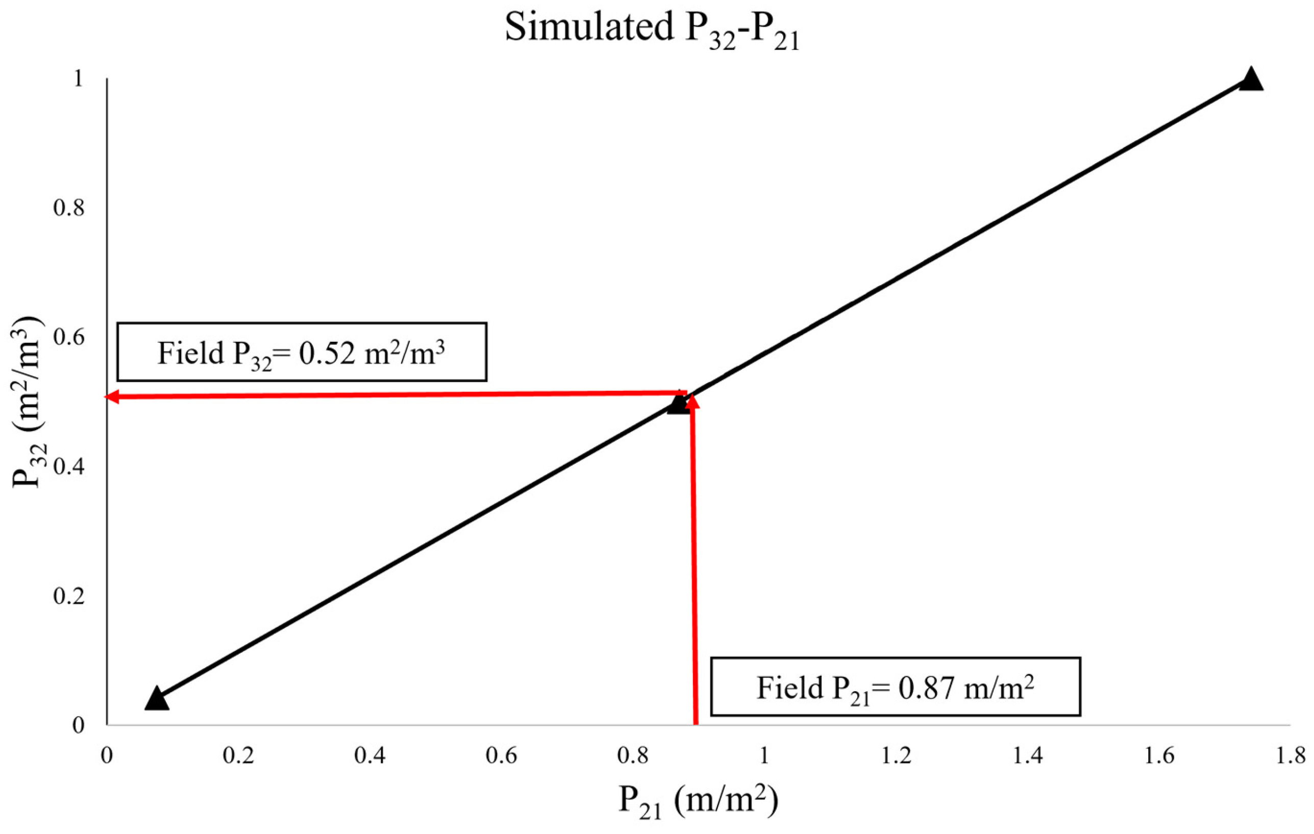
Figure 6.
DFN model in Fracman [37]: (a) 3D DFN model, and (b) Fracture traces on a 2D longitudinal section.
Figure 6.
DFN model in Fracman [37]: (a) 3D DFN model, and (b) Fracture traces on a 2D longitudinal section.
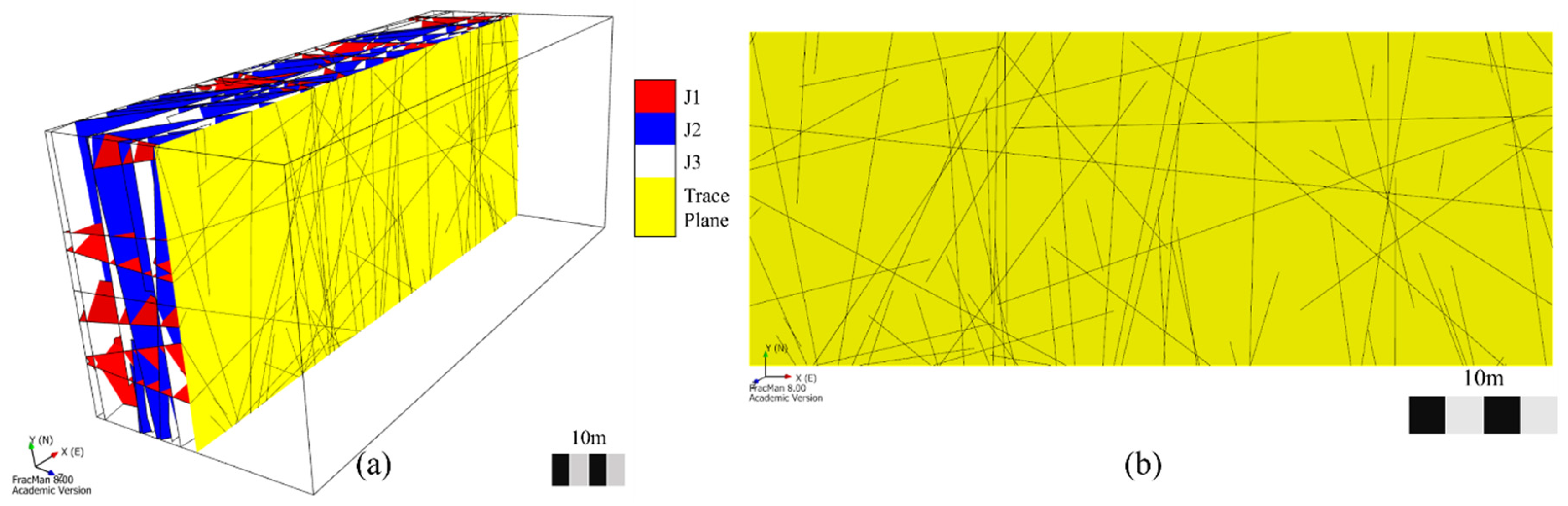
Figure 7.
Fracture orientation comparison using DIPS [38]: (a) Stereonet with input orientation, (b) Stereonet with DFN generated fractures.
Figure 7.
Fracture orientation comparison using DIPS [38]: (a) Stereonet with input orientation, (b) Stereonet with DFN generated fractures.
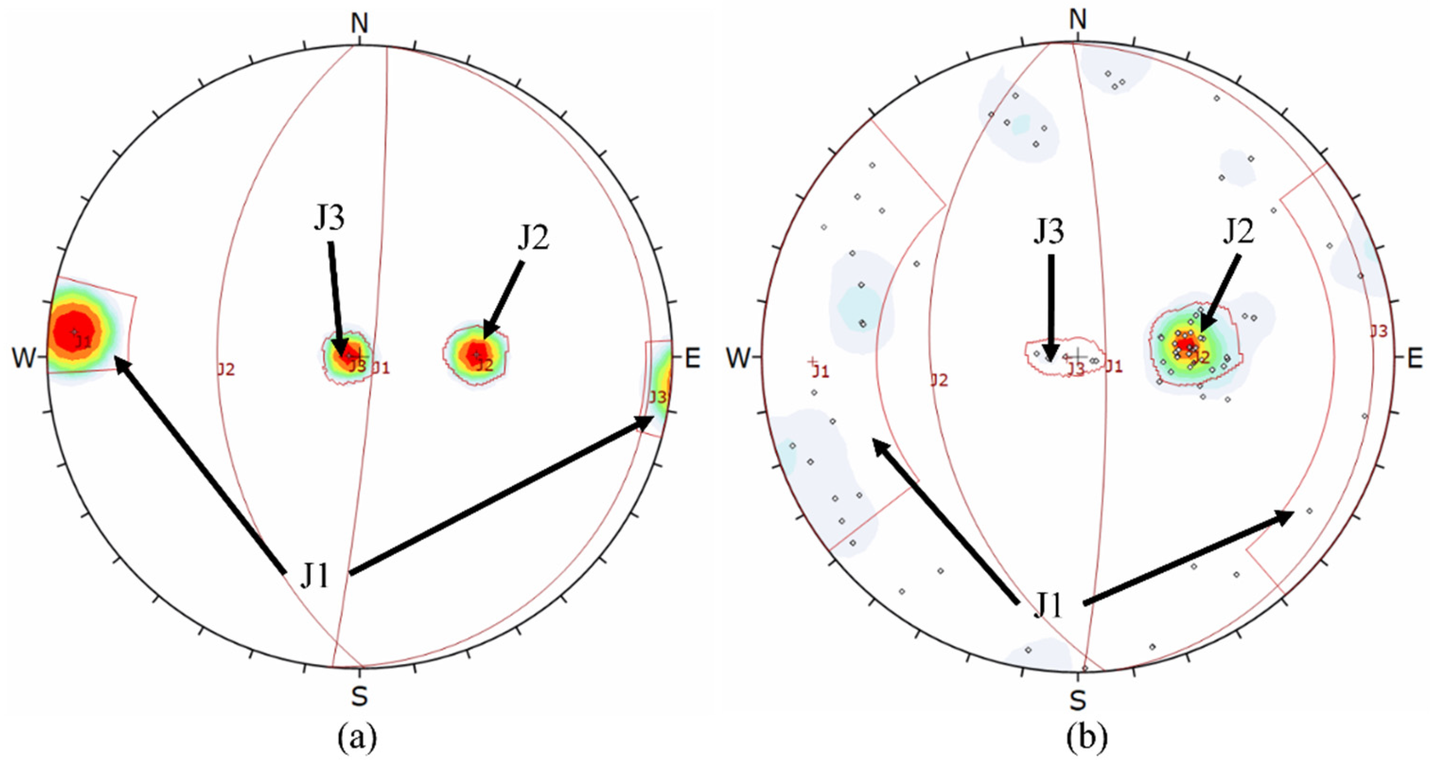
Figure 8.
Single blasthole bench blast without DFN (red boundary represents blasting pressure boundary).
Figure 8.
Single blasthole bench blast without DFN (red boundary represents blasting pressure boundary).
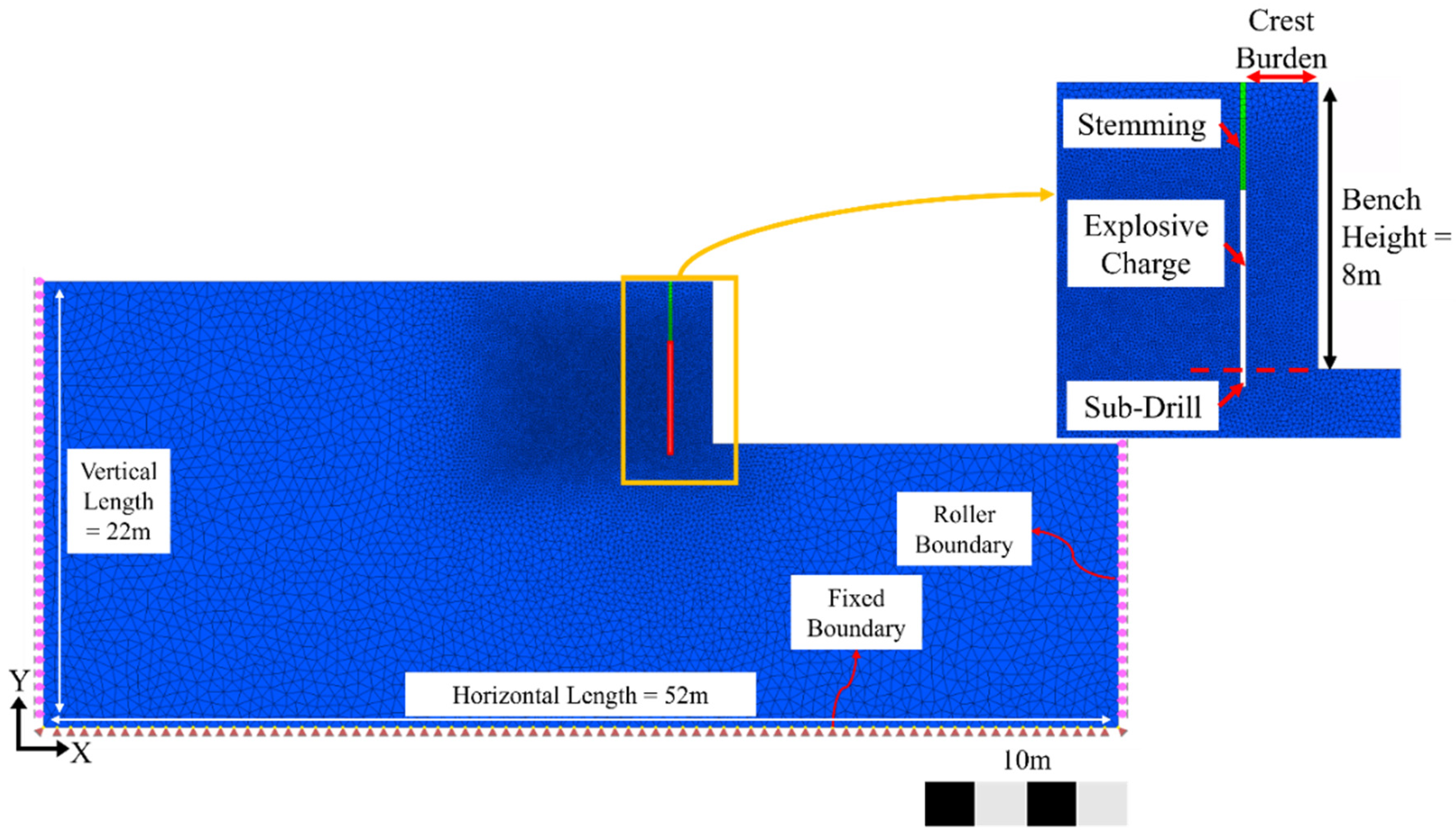
Figure 9.
Single blasthole bench blast with DFN traces.
Figure 10.
Detonation and gas pressure-time curves and their combination pressure-time curve applied to blasthole boundary.
Figure 10.
Detonation and gas pressure-time curves and their combination pressure-time curve applied to blasthole boundary.
Figure 11.
Total areas selected for (a) Scenario 1 and (b) Scenario 2 (DFN is shown with red straight lines).
Figure 11.
Total areas selected for (a) Scenario 1 and (b) Scenario 2 (DFN is shown with red straight lines).
Figure 12.
Example of yielded elements for (a) Scenario 1 and (b) Scenario 2.
Figure 13.
Scenario 1 blasting process: (a) Fractures reached free face, (b) Fragmentation and movement, and (c) Muckpile formation.
Figure 13.
Scenario 1 blasting process: (a) Fractures reached free face, (b) Fragmentation and movement, and (c) Muckpile formation.
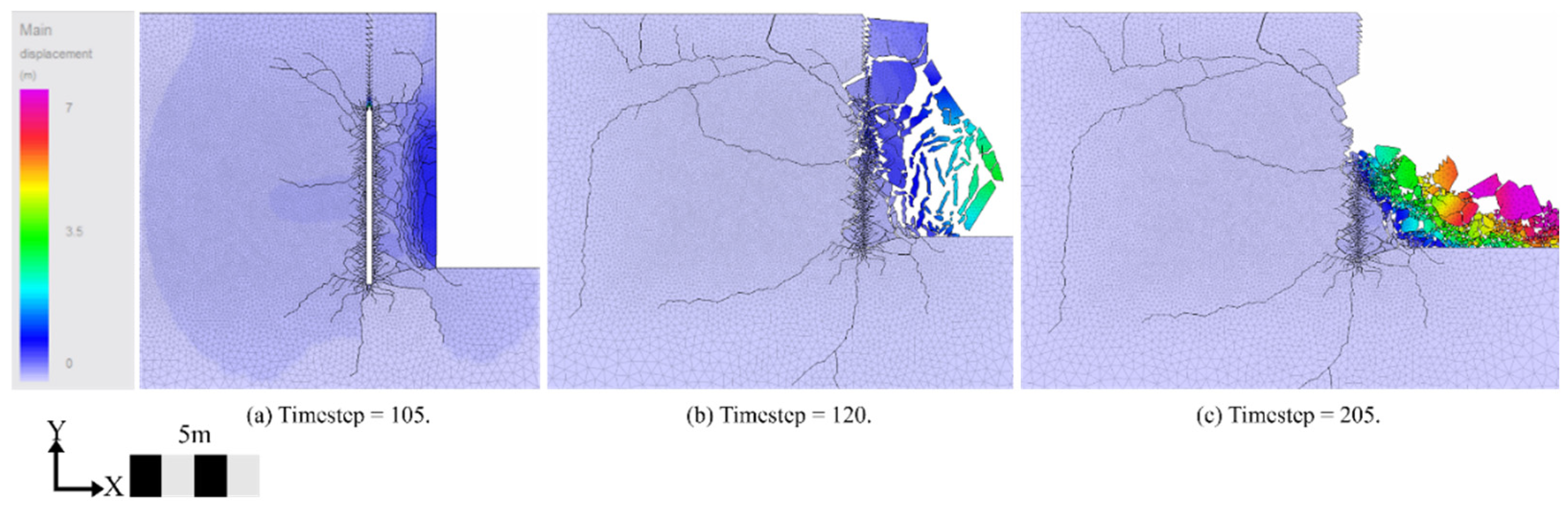
Figure 14.
Scenario 2 blasting process: (a) Fractures reached bench open surface, (b) Fragmentation and movement, and (c) Muckpile formation.
Figure 14.
Scenario 2 blasting process: (a) Fractures reached bench open surface, (b) Fragmentation and movement, and (c) Muckpile formation.

| Measurement Dimension | Measure Type | |||||
| 0 | 1 | 2 | 3 | |||
| Sample Dimension |
1 | P10 Quantity of fractures per unit length of borehole. |
P11 Length of fractures per unit length. |
Linear | ||
| 2 | P20 Quantity of fractures per unit area. |
P21 Length of fractures per unit area. |
P22 Area of fractures per area. |
Areal | ||
| 3 | P30 Quantity of fractures per unit volume. |
P32 Area of fractures per unit volume. |
P33 Volume of fractures per unit volume. |
Volumetric | ||
| Term | Density | Intensity | Porosity | |||
Table 2.
Mechanical properties of the rock [28].
Table 2.
Mechanical properties of the rock [28].
| Parameters | Value | Symbol |
|---|---|---|
| Density (kg/m3) | 2660 | r |
| Young’s Modulus (GPa) | 52 | E |
| Poisson’s Ratio | 0.16 | υ |
| Cohesion (MPa) | 33 | C |
| Tensile Strength (MPa) | 17 | ft |
| Constitutive law | Plane strain |
Table 3.
Mechanical properties of the copper tube [36].
Table 3.
Mechanical properties of the copper tube [36].
| Parameters | Value | Symbol |
|---|---|---|
| Density (kg/m3) | 833 | rCu |
| Young’s Modulus (GPa) | 13.8 | ECu |
| Poisson’s Ratio | 0.35 | υCu |
| Cohesion (MPa) | 20 | CCu |
| Tensile Strength (MPa) | 400 | ftCu |
| Constitutive law | Plane strain |
Table 4.
Peak pressure results obtained from numerical and experimental procedures.
| Monitoring Point | Distance from blasthole (mm) | Experimental Peak Pressure (MPa) [28,35] | Numerical Peak Pressure (MPa) [28] | Numerical Peak Pressure (MPa) (this paper) |
|---|---|---|---|---|
| 1 | 11.0 | 52.1 | 51.2 | 52.3 |
| 2 | 22.5 | 23.8 | 33.8 | 26.6 |
| 3 | 44.0 | 15.8 | 19.8 | 17.7 |
Table 5.
Number of radial fractures obtained from numerical and experimental procedures.
| Experimental [28,35] | Numerical [28] | Numerical (this paper) |
|---|---|---|
| 9 | 8 | 9 |
Table 6.
Fracture sets orientation and input data for DFN model generation.
| Parameters | Fracture Set | Value |
|---|---|---|
| Orientation (Dip/Dip Direction) (°) | J1 | 85/095 |
| J2 | 41/269 | |
| J3 | 04/096 | |
| Fisher’s K | J1/J2/J3 | 60 |
| P32 (1/m) | J1/J2/J3 | 0.52 |
Table 7.
Fracture orientation comparison.
| Input Orientation | DFN Generated Orientation | Variation (%) | ||||
| Fracture Sets | Dip (°) | Dip Direction (°) | Dip (°) | Dip Direction (°) | Dip | Dip Direction |
| J1 | 85 | 095 | 80 | 089 | 5.88 | 6.32 |
| J2 | 41 | 269 | 40 | 265 | 2.44 | 1.49 |
| J3 | 04 | 096 | 04 | 083 | 0.00 | 13.54 |
Table 8.
Rock, explosive and DFN properties for FDEM simulations.
| Material | Parameters | Value | Units | Symbol |
|---|---|---|---|---|
| Rock | Density | 2700 | kg/m3 | r |
| Young’s Modulus | 60 | GPa | E | |
| Poisson’s Ratio | 0.25 | υ | ||
| Uniaxial Compressive Strength | 110 | MPa | UCS | |
| Viscous Damping | 1 | |||
| Cohesion1 | 22 | MPa | C | |
| Tensile Strength2 | 11 | MPa | ft | |
| Friction Coefficient | 0.47 | fr | ||
| Friction Energy Mode I | 31 | N/m | GI | |
| Friction Energy Mode II | 310 | N/m | GII | |
| Constitutive Law | Plane strain | |||
| Explosive | Explosive Type | Heavy ANFO | ||
| Density | 1200 | kg/m3 | re | |
| Velocity of detonation | 5000 | m/s | VOD | |
| DFN | Fracture type | Broken | ||
| Friction Coefficient | 0.73 | |||
1 Cohesion is 20% of the UCS. 2 Tensile strength is 10% of UCS.
Table 9.
Blast design properties.
| Parameters | Value | Units |
|---|---|---|
| Crest Burden | 2 | m |
| Stemming Length | 3 | m |
| Charge Length | 5 | m |
| Subdrill | 0.5 | m |
| Blasthole diameter | 165 | mm |
| Bench height1 | 8 | m |
1 Stiffness ratio (bench height divided by crest burden) is 4.
Table 10.
Damage intensity values for the scenarios.
| Scenario | Damage intensity (Di) |
|---|---|
| 1: Blast without DFN | 0.26 |
| 2: Blast with DFN | 0.15 |
Disclaimer/Publisher’s Note: The statements, opinions and data contained in all publications are solely those of the individual author(s) and contributor(s) and not of MDPI and/or the editor(s). MDPI and/or the editor(s) disclaim responsibility for any injury to people or property resulting from any ideas, methods, instructions or products referred to in the content. |
© 2024 by the authors. Licensee MDPI, Basel, Switzerland. This article is an open access article distributed under the terms and conditions of the Creative Commons Attribution (CC BY) license (http://creativecommons.org/licenses/by/4.0/).
Copyright: This open access article is published under a Creative Commons CC BY 4.0 license, which permit the free download, distribution, and reuse, provided that the author and preprint are cited in any reuse.


