
Submitted:
10 October 2024
Posted:
11 October 2024
You are already at the latest version
Abstract
Background: wildfire modelers rely on Monte-Carlo simulations of wildland fire to produce burn-probability maps. These simulations are computationally expensive. Methods: we study the application of Importance Sampling to accelerating the estimation of burn probability maps, using L2 distance as the metric of deviation. Results: assuming a large area of interest, we prove that the optimal proposal distribution re-weights the probability of ignitions by the square root of expected burned area divided by expected computational cost, then generalize these results to assets-weighted L2 distance. We also propose a practical approach to searching for a good proposal distribution. Conclusion: these findings contribute quantitative methods for optimizing the precision/computation ratio of wildfire Monte Carlo simulations without biasing results, offer a principled conceptual framework for justifying and reasoning about other computational shortcuts, and can be readily generalized to a broader spectrum of simulation-based risk modeling.
Keywords:
Monte Carlo simulations
; wildfire
; risk modeling
; burn probability
; variance reduction
; sampling error
1. Introduction
Monte Carlo simulations [1] are an approach to studying random processes by drawing samples from them. This approach has often been applied to studying the potential impacts of wildfire [2]: burn probability maps can be produced from Monte Carlo simulations, by averaging the burned areas of many randomly ignited fires simulated by a wildfire behavior model [3].
Simulating a large number of fires is required to ensure that the Monte Carlo estimator converges to an asymptotic value; otherwise, running the simulations again may produce a significantly different result. This random variability is known as the variance of the Monte Carlo estimator. Reducing the variance is required for making the estimation precise.
Importance Sampling is a general strategy for reducing the computational cost of Monte Carlo simulations. Importance Sampling redistributes the sampling probability of simulation outcomes, while inversely scaling their contribution to simulation results. This preserves the expected value of the Monte Carlo estimator while altering its variance, enabling faster convergence to the asymptotic estimand. In the case of wildfire simulations, importance sampling boosts or depresses the probability that some fires will be simulated, and accordingly decreases or increases their contribution to the aggregated simulation results. In [1] importance sampling is described as “the most fundamental variance reduction technique”. Therefore, it appears important for fire modelers to consider using Importance Sampling in their simulations; this article aims to help them understand its underlying principles, assess its potential benefits, and implement it when they are significant.
Importance Sampling has been used for sub-aspects of wildfire simulation. [4] have studied the use of Importance Sampling for data assimilation. [5] use Importance Sampling as part of the simulation of spotting behavior. We know of no academic study of Importance Sampling for accelerating the estimation of risk maps.
This paper is structured as follows. Section 2 will develop the conceptual methods introduced by this paper: this will mostly consist of framing the problem of computational efficiency in wildfire simulations, through concepts like cost-to-precision ratio and efficiency gain, introducing a generalized notion of variance (based on the norm) suited to estimating burn-probability maps (Section 2.1, Equation (2)), then recalling the definition of Importance Sampling (Section 2.4) as a technique for accelerating estimator convergence in Monte-Carlo simulations, adapting it to the context of wildfire simulations with variance, calculating its performance characteristics, considering various generalizations, and suggesting approaches to implementing the approach (Section 2.12). Section 3 will illustrate these methods will various case studies. Section 4 discusses the limitations of this approach. Table 1 summarizes the symbols most commonly encountered in formulas; their meaning will be defined in Section 2.
2. Materials and Methods
This analysis is conducted in the context of estimating burn probability maps over a large Area of Interest .
2.1. Background: Mean, Variance and Precision of Random Maps
For measuring the difference between multidimensional outputs like burn-probability maps, we use the norm , defined by the spatial integral:
The distance between two maps and is then .
We generalize the notion of variance from random numbers to random maps as follows. If is a random map, then we define the variance of to be:
Note that this can also be expressed in terms of pointwise variances - for each spatial location s, is a random number of variance , and we have
Many properties of scalar variance are retained: variance is additive on independent variables, and a random variable is constant if and only if its variance is zero.
A useful related concept is the precision, defined as the inverse variance:
Aiming for low variance is equivalent to aiming for high precision.
2.2. Mean Estimation from Monte Carlo Simulations
Assume that we want to estimate the unknown expectation of a distribution of interest, represented by a random map . (Note that itself is a map, not a number). When all we know about is how to draw samples from it, a Monte Carlo simulation lets us estimate by drawing many i.i.d samples , and computing their empirical mean :
Expectation being linear, it is easily seen that . The point of drawing a large number of samples N is to increase the precision of that estimation, so that we can rely on . Indeed, from the properties of variance, the variance and precision of are related to the sample size N as follows:
The precision formula is insightful: we can think of each sample contributing to estimator precision. Thus, can be viewed as a precision per sample performance characteristic of our sampling distribution.
Assume now that with each sample is associated a computational cost of drawing it - typically is expressed in computer time. For example, in wildfire simulation, large fires are often more costly to simulate than small fires. Then the cost of drawing a large number N of i.i.d samples will be approximately . This motivates the following concept of cost-to-precision ratio, which quantifies the overhead of our estimator:
2.3. Burn-Probability Maps from Monte Carlo Simulations
We assume the following structure for how simulations run. Each simulation k draws initial conditions (typically, encompasses the space-time location of ignition, and the surrounding weather conditions), from which a fire is simulated to yield a binary burn map , in which
Thus, each is a Bernoulli random variable, and its expectation is the probability that one simulation burns location s.
We assume that the are sampled i.i.d., and so will write to denote a random variable representing their common distribution. Likewise for the .
The goal of the simulations is to estimate the expected burn probability, which is defined as the expectation of the burn map, therefore yielding a map of burn probabilities:
That estimation is typically done by using the Crude Monte Carlo (CMC) estimator , which draws a large number N of fires and computes the average of the :
Because each is a Bernoulli random variable (taking only 0 and 1 as values), has an interesting expression in terms of expected fire size:
in which is the (random) fire size (say, in or acres, or whatever unit was chosen for ). More precisely, is the area burned by the random fire within the AOI .
The above derivation relies on , which we now prove. Denoting the (random) set of locations burned by a simulated fire, and observing that , we have:
Another insightful relationship is that the expected fire size is the spatial integral of the expected burn probability:
Finally, we note a useful approximation. In the common settings where the burn probabilities are low (each location s is burned only by a small minority of simulated fires), then implies that , and since it follows that , and
In other words, the variance of the binary burn map is well approximated by the expected fire size.
2.4. Using Importance Sampling for Reducing the Cost-to-Precision Ratio
We now borrow from the concept of Importance Sampling from the generic Monte Carlo literature [1]. This will enable us to design other Monte Carlo estimators for the burn-probability , with lower cost-to-precision ratio than the CMC estimator, thus requiring less computation to achieve convergence.
Denote the “natural” probability distribution from which simulated fires are sampled (i.e. ), which is hopefully representative of real-world fire occurrence. The CMC estimator consists of drawing samples from p then averaging the maps. Importance Sampling modifies this procedure by drawing samples from another distribution (called the proposal distribution) and reweighting the samples to remain representative of p, yielding the Likelihood Ratio estimator1:
in which we defined the importance weight as the ratio of probabilities:
It is easily verified that this change of estimator preserves the expected value:
What can make this new estimator valuable is its variance:
The approach of Importance Sampling consists of seeking a proposal distribution q which minimizes the cost-to-precision ratio . When the cost is constant, this amounts to minimizing variance, in which case a classical result of the Monte Carlo literature says that the optimal proposal distribution and the corresponding variance are given by:
This is an improvement over because , as can be seen for example by applying Jensen’s inequality [6].
We place ourselves in a more general context, corresponding to a non-constant cost . More precisely, we will assume:
- the cost being a function of the simulated fire:
The cost-to-precision ratio achieved by a proposal distribution q is then:
For practical purposes, we often need to know the weight function only up to a proportionality constant. For example, we can compute the efficiency gain of proposal distribution q as:
The efficiency gain quantifies how the cost-to-precision ratio improves from the Crude Monte Carlo estimator () to Importance Sampling (). We see that replacing w by in Equation (22) leaves the result unchanged, because the constant gets simplified away in the denominator. Likewise for equation .
2.5. Computing Sampling Frequency Multipliers
To better understand the effect of Importance Sampling with some reweighting function , we introduce the notion of frequency multipliers, which describe how the sampling frequencies of simulated fires change when we use Importance Sampling.
The same-cost frequency multipliers correspond to the following procedure. Assume that we initially planned to simulate N fires with the natural distribution p, which means an expected computational cost of . We then choose to adopt Importance Sampling with reweighting function w (or equivalently, with proposal density q), and consequently adjust the number of simulated fires to to keep the same expected computational cost, i.e. . For any potential simulated fire b, we can then ask the question: how much more frequently does b get drawn by Importance Sampling than by our original sampling design? This number is the same-cost frequency multiplier of b, and can be computed as:
Similarly, we can conceive of the same-precision frequency multiplier. Then the number of simulated fires is adjusted from N to so that precision remains the same, i.e. . Then the frequency multiplier gets computed as:
Confusion pitfall: note that the frequency multipliers are inversely proportional to the reweighting function w.
2.6. The Optimal Proposal Distribution
This section shows that there is an optimal proposal distribution, and that it can be described quantitatively. Applying the probabilistic Cauchy-Schwarz inequality (Appendix A.2) to Equation (2.4) yields an expression for the optimal proposal distribution and its cost-to-precision ratio:
2.7. Application to Burn-Probability Maps
In the case of burn maps, recalling that , it follows that
In other words, the best proposal distribution reweights the probability of each fire by the square root of its size-to-cost ratio. Two special cases of cost functions stand out:
- when the cost of simulating a fire is proportional to its size, then Importance Sampling makes no difference: the initial distribution is already the optimal proposal distribution;
- when the cost of simulating a fire is constant, then the optimal proposal distribution reweights the probability of each fire by the square root of its size.
It is also interesting to consider a mixture of these cases. The cost function can be modeled as the sum of a constant term and a term proportional to fire size: . For very large fires (), the size-to-cost ratio will be very close to 1, such that no reweighting will occur: large fires will be sampled according to their natural distribution. For very small fires (), the size-to-cost ratio will be very small, such that these fires will have virtually no chance of being sampled; and since they do not contribute much to the mean, the weight will not be high enough to compensate this sampling scarcity. This provides a principled justification for the common heuristic of dispensing with simulating small fires: provided that is not too large, that heuristic is very close to the optimal proposal distribution.
To further illustrate this phenomenon, Figure 1 displays the maximum potential efficiency gain (Equation (27)) for an imaginary model in which the cost c is determined by the fire size A as , based on the distribution of fire sizes recorded in the Fire Occurrence Database [7]. When the constant term is high (high ), a lot of efficiency can be gained by reducing the sampling frequency of small fires. When the cost is a superlinear function of size (), efficiency can be gained by reducing the sampling frequency of large fires.
2.8. Generalization: Optimal Proposal Distribution for Ignitions
We now assume that we do not have enough mastery over to find the optimal proposal distribution . Instead, we restrict ourselves to seeking a proposal distribution for the ignition , such that is of the form:
This decomposition is consistent with the idea that we’re going to change the distribution of ignitions without changing the fire spread algorithm itself. For example, Section 3.4 will change the sampling distribution of ignitions based on fire duration. Under this constraint, the cost-to-precision ratio of the proposal distribution can then be expressed as:
in which the functions compute the conditional expectation of fire size and computational cost:
The proof to Equation (25) can then be generalized to show that the optimal proposal distribution is given by:
It can then be seen that yields the following density and cost-to-precision ratio:
Note that any random variable can be chosen for these results to apply. Here we have described as the “ignition” or “initial conditions”, but it can be any predictor of fire size and simulation cost. Two extreme cases of are noteworthy:
- If is fully determined by (deterministic simulation), then we recover .
- If is uninformative (independent) w.r.t , then we obtain a no-progress optimum of .
2.9. Generalization: Impact-Weighted Distance
An interesting generalization consists of using another measure than area for computing distances, by introducing a density function which quantifies the “value” or “concern” per unit area:
Then all the results of the previous section apply (with being replaced by in integrals), except that the interpretation changes: quantities like , and no longer measure fire size, but burned value. In particular, when using the optimal proposal distribution for importance sampling, each fire sees its sampling probability reweighted by the square root of its burned value/simulation cost ratio.
Weighting by value instead of area can dramatically change the optimal proposal distribution. It can boost the probability of sampling small fires near valuable assets, while depressing the probability of large fires in low-concern areas. From this perspective, “Area of Interest” takes on a very precise meaning: the set of locations s where .
The choice of value measure depends on how the burn-probability map will be used: where do we want precision? For example, the burn-probability maps might be used to plot the risk to properties and infrastructure, and also be aggregated to estimate GHG and smoke emissions. To that end, a good value function could place strong measure on properties and infrastructure, and mix that with small measure on fuel loads (the latter do not need as high a measure because emissions are destined to be aggregated, which already reduces variance).
2.10. Generalization: Non-Geographic Maps and Non-Binary Outcomes
Another way to understand Section 2.9 is to pretend that the variable ranges not over geographic space, but over “assets space”. Attentive readers may have noticed that nothing in the above analysis is specific to the spatial nature of the set . We can conceive of other type of burn-probability maps: for example, may be:
- a space-time region, like or , in which ;
- a combination of geographic space and fire severity buckets, like ;
- a combination of geographic space and paired scenario outcomes, like:
The above paragraph generalizes , that is the domain of function ; we can also generalize its codomain, that is the simulation outcomes. In particular:
- need not be binary: for example, might be a density of greenhouse-gas emissions;
- need not be about fire.
What matters for the analysis of this article to apply is that the outcomes be aggregated by averaging, and for the Poisson process approximation to be valid (Section 2.14). Note that when the outcomes are not binary, can no longer be interpreted as the impacted area, i.e. Equation (11) () no longer holds.
2.11. Variant: Sampling from a Poisson Point Process
The above analysis assumes that the number of fires is fixed, and that the fires are sampled i.i.d. A variant of this sampling scheme is to sample from a Poisson Point Process (PPP) [8] instead: this is equivalent to saying that the number of fires is no longer fixed, but follows a Poisson distribution. The PPP can be appealing because it is algorithmically convenient (subregions of space-time can be sampled independently) and yields mathematical simplifications, as we will see below.
In the context of a PPP, a random number of fires are sampled, and the Likelihood Ratio Estimator, which we now denote , is virtually unchanged:
By writing , it is easily verified that the mean of this estimator is correct: .
An interesting aspect of the PPP is that the variance approximation of Equation (19) becomes exact2, such that:
It follows that the results of the previous section about the optimal proposal distribution and cost-to-precision ratio remain unchanged.
2.12. Practical Implementation
The previous sections described the optimal proposal distribution which can be achieved with perfect knowledge of the impact and cost functions and . In practice, these functions will be unknown, so that Equation (32) is not applicable. Instead, we suggest using a calibration approach to estimate an approximately optimal proposal distribution, through the following steps:
- Run simulations to draw a sample of ignition and simulated fire , yielding an empirical distribution which we will represent by the random variables .
- Design a parametric family of weights functions .
-
Find the optimal parameter vector by solving the following optimization problem, inspired by Equation (2.4):If does not yield a significant improvement compared to , try a new family of weights functions, or abandon Importance Sampling.
- Adopt as the proposal distribution for Importance Sampling.
Care should be taken to appropriately constrain the parametric family to avoid any problem of identifiability, since the objective function in Equation (37) will yield exactly the same score for a reweighting function w and a scaled variant : therefore, the family of reweighting functions must not be stable by rescaling. It might also be sensible to add a regularization term to the objective function.
In addition to using a parametric family, it can be sensible to use a curve-fitting approach: one can compute the weights which are optimal for the (discrete) empirical distribution, then use some interpolation algorithm to derive a continuous weight function, like a supervised learning algorithm or nearest-neighbor method [9].
2.13. Analysis of Geographic Inequalities in Precision
The above analysis describes how to optimize the global precision (in the sense of the norm); however, doing so might alter the relative geographic distribution of local precision across the map. In particular, we can expect that this optimization will favor absolute precision over relative precision, spending the computational cost mostly in areas of high burn probability. Section 3.3 provides an example that illustrates this phenomenon.
2.14. Justifying the Poisson Process Approximation
The proof to Equation (25) relies on the Poisson process approximation (Equation (19)), which we now justify. It follows from Equation (18) that is the smallest possible value for . Therefore, it is enough to show that . We suggest that this generally holds, by considering the case where is spatially uniform. Denoting the total area, we then have , and is equivalent to the following condition on the burned fraction:
... which will be the case in the typical situation where the burned fraction is almost certainly much smaller than 1. The general phenomenon here is that becomes an insignificant component of variance as the AOI is made much larger than the fires; this corresponds to the Binomial-to-Poisson approximation we showed in a previous paper [10].
Another perspective to shed light on this phenomenon is that making the AOI very large means that the sampling procedure behaves like a Poisson Point Process (Section 2.11) in any minority subregion of the AOI; then Equation (36) holds approximately. This is the same phenomenon as the Binomial-to-Poisson approximation: the number of points drawn in a small subregion follows a Binomial distribution with a small probability parameter, which is well approximated by a Poisson distribution.
2.15. Importance Sampling versus Stratified or Neglected Ignitions
Stratification [11] is another strategy for reducing the variance of Monte Carlo simulations. In the case of burn-probability estimation, stratification might consist of partitioning the set of possible ignitions into several subsets (for example, low-risk and high-risk), and simulating more fire seasons in some subsets than others. The burn probability maps from each subset are then combined by a weighted sum, the weights being inversely proportional to the number of fire seasons. A similar strategy consists of dividing the space of ignitions between a low-risk and high-risk subsets, and simulating only the high-risk subset, thus neglecting the other.
Observe that both strategies are highly similar to a special case of Importance Sampling, in which the weight function is piecewise constant. Therefore, Importance Sampling is useful for reasoning about these other strategies, and provides an upper bound to their potential efficiency gains.
3. Results
We illustrate the above methods by applying them to an existing dataset of results from a wildfire Monte-Carlo simulation. We will implement various forms of Importance Sampling, estimate the efficiency gains, and discuss the trade-offs. Due to limited access to computed resources, we did not run new simulations based on the reweighted sampling scheme; instead, we use simulation results that were drawn without Importance Sampling, and quantity the efficiency gains that would have been obtained by implementing Importance Sampling.
3.1. Simulation Design and Results
The dataset of simulated fires studied here was produced as part of the 3rd version of the FireFactor project [12]. We will not try to discuss the validity and implementation details of these simulations here - that would require its own publication - and we will instead focus solely on aspect relevant to our study of Importance Sampling. 800 repetitions of the 13 years from 2011 to 2023 were simulated with historical weather. The ignition locations, times, and fire durations were randomly drawn as a Poisson Point Process [8], following a density function that was influenced by predictor variables such as fuel type, weather, distance to built areas, and a spatial density of ignitions derived from historical data. Compared to previous versions of the FireFactor project, a salient feature of this version is a heavy tail of fire durations, in an attempt to represent the occurrence of very large fires more faithfully. As already noted, we did not use Importance Sampling in these simulations.
This simulation procedure produced a dataset of approximately 31.7 million simulated fires. Because this size of data was impractical for the experiments described below, we thinned this dataset into a random sub-sample of approximately 2.7 million fires: for each fire, we independently drew a random binary variable to determine whether it would be selected in the sub-sample. To improve precision, the larger fires had a higher probability of being selected in the sub-sample4. Based on a rough examination of a fire size histogram and some judgement-based trial and error, the selection probability was chosen to be the following function of the fire size A:
Thus, the selection probability was almost uniform when (809.3 ha), approximately proportional to when , and saturating to 1 when (12140.6 ha).
Denote the original sample of 31.7 million fires, and the thinned sub-sample. Then, for any function , we will be able to approximate the sum of the as follows:
in which the symbol denotes equality in expectation, and is the appropriate subsampling weight derived from the selection probability:
3.2. Maximum Potential Efficiency Gain
By applying Equation (27) to the dataset described in Section 3.1, we obtained (standard error ). The standard error was estimated by bootstrap-resampling [13] using 100 bootstrap replications.
The above result is an upper bound on the efficiency gain that can be obtained by Importance Sampling; however, it does not tell us what reweighting function to use in order to approach that upper bound. The next section will explore various reweighting strategies.
3.3. Reweighting Pyromes Uniformly
We start with a reweighting function that is constant within each pyrome. The approach is therefore similar to stratifying (Section 2.15) by pyrome. Pyromes [14] are a spatial partition of the Conterminous United States into 128 areas of relatively homogeneous fire occurrence characteristics. This reweighting strategy means that instead of simulating the same number of fire seasons in all pyromes, we simulate more fire seasons in some pyromes than others; however, the relative frequencies of simulated fires ignited within a given pyrome remain the same.
By applying Equation (33) with variable I defined as the pyrome of ignition, we know the importance weight for a pyrome is proportional to , the square root of expected cost divided by expected burned area in that pyrome. Thus, we estimated and for each pyrome I, yielding the optimal weighting function, up to some proportionality constant. Using Equation (22), we computed the efficiency gain , yielding a value of .
We then assessed the geographic inequality in precision implied by this reweighting scheme (Section 2.13). To do so, we computed the same-cost frequency multipliers (Equation (23)), telling us how the number of simulated seasons in each pyrome has increased or decreased. All else being equal, precision is proportional to the number of simulated years, therefore the gain in precision within each pyrome is equal to this multiplier. Table 2 shows the multipliers for each pyrome, along with some other descriptive statistics; these numbers are plotted in Figure 2. We see that most pyromes have a multiplier between 0.7 and 1.3, with a few as low as 0.4 and none higher than 2.
In our opinion from looking at these results, this particular reweighting scheme is more trouble than it is worth: the efficiency gain is rather small, and the reduce precision in some pyromes is concerning.
3.4. Duration-Based Parametric Reweighting in Pyrome 33
As another example, we restrict our attention to only one pyrome and use a parametric weight function (as suggested by Section 2.12) based on simulated fire duration. The assumption here is that the simulated fire duration is randomly drawn at the same time as the ignition location (before the fire is simulated), and that we can oversample or undersample fires based on their duration.
The pyrome under consideration is Pyrome 33 (South Central California Foothills and Coastal Mountains). For this pyrome, we computed (Equation (27)) a maximum potential efficiency gain of .
We will use a parametric reweighting function, of the form:
in which is a parameter controlling how short fires will get over-sampled () or under-sampled () by Importance Sampling.
To estimate the optimal value , we used the scipy.optimize.minimize function of the SciPy library [15] to solve the following optimization problem, corresponding to Equation (37):
in which k indexes the simulated fires of the calibration dataset, is the duration of the k-th simulated fire, and is the subsampling weight (see Equation (41)).
The best-fitting parameter value is , achieving an efficiency gain of 1.25 (as computed by Equation (22)). Shorter fires get a smaller weight () which means that Importance Sampling will improve efficiency by over-representing them. The curve in Figure 3 shows how Importance Sampling alters the sampling frequency of fires under this reweighting function, by displaying the same-cost frequency multipliers (Equation (23)) corresponding to , along with a point cloud of the frequency multipliers yielded by the best possible reweighting scheme (given by Equation (25)).
A side effect of the reweighted function fitted above is that it increases the sampling frequency of very short fires. There is cause to be unsatisfied with this, in particular because simulating a very large number of tiny fires can make the results unwieldy in ways not captured by our cost function. To address this limitation, we now fit a more refined reweighting function, expressed as:
The above function is more flexible, having 4 parameters instead of 1; in particular, the duration lengthscales are no longer fixed, thanks to the parameters. We fitted this function with initial parameters : in practice, this means that influence short fires while influence long fires. The best-fit values were , achieving an efficiency gain of 1.27 (confirmed with K-fold cross-validation). Note that , thus reducing the sampling frequency of very short fires. Figure 4 displays the fitted frequency multipliers: in summary, Importance Sampling in this case will increase the sampling frequency of medium-duration fires, at the expense of low-duration and high-duration fires.
3.5. Fitting a Machine-Learning Model to Empirical Optimal Weights
We now illustrate the last suggestion of Section 2.12: fitting a supervised learning to the optimal weights derived from the empirical sample. Using the dataset of 2.7 million simulated fires described in Section 3.1, we trained a gradient-boosted regression tree algorithm [9] to predict the optimal weight (computed from the empirical sample using Equation (25)). More precisely, we used the HistGradientBoostingRegressor class of the Scikit-Learn library [16], which is inspired by LightGBM [17]. We used as the target variable, and we weighted samples by fire size. As predictor variables, we used the fire duration, pyrome number, ignition-point fuel model number, ignition-time ERC percentile, some fire behavior metrics (rate of spread, reaction intensity in , fire-line intensity in kW/m) derived from the fuel model in reference weather conditions5 using the Rothermel model [18], and spatial coordinates of ignition point .
We fitted two models, differing only in which subset of predictor variables was used:
- Model A: used all predictor variables listed above.
- Model B: used all predictor variables except for the spatial coordinates .
The models were tested by a method similar to K-fold cross-validation: training on a random subset of 70% of the fires, computing the efficiency gain on the remaining 30%, repeating this procedure 30 times and computing the mean and standard deviation of the efficiency gain. The test performance of the model is summarized by Table 3. We see that Model A achieves a much higher efficiency gain than Model B, revealing that it learns fine-grained spatial features from the spatial coordinates of ignition. While its superior efficiency gain is appealing, we are wary of using Model A, because of the subtle potential side effects of having estimator precision that varies at fine spatial scales.
4. Discussion
Perhaps the most questionable aspect of these methods is the use of as the metric of deviation. While this choice is mathematically convenient, and has various theoretical justifications, it may create geographic disparities in precision, and excessively favor absolute precision over relative precision (as noted in Section 2.13).
When the computational cost of a simulated fire is asymptotically a super-linear function of its size, then Importance Sampling will reduce the sampling frequency of large fires (Section 2.7). This is unintuitive, and can be problematic: the largest fires are typically those we are most interested in. Reducing the sampling frequency of large fires may improve precision in the sense of , but it might at the same time conflict with other precision objectives. This issue can be mitigated in several ways:
- by weighting the metric by value (Section 2.9), e.g. by giving more importance of Highly Valued Resources and Assets;
- by including non-geographic outcomes like burn severity (Section 2.10) and weighting them unevenly;
- by constraining the family of reweighting functions under consideration to be uniform in the tail of large fires.
Consequently, the main recommendation of this article is to consider using some form of importance sampling, not necessarily the one which is optimal in the sense of convergence. We find the approach most promising for reducing the sampling frequency of many small inconsequential fires in situations where the simulation pipeline makes them disproportionately costly.
To make such approaches practical, we recommend that wildland fire simulation software enable users to provide weights alongside ignitions, these weights being taken into account for aggregating simulation results into outputs. It should be immaterial whether such weights originate from importance sampling or similar techniques like stratified sampling.
5. Conclusions
This article has studied the application of Importance Sampling to Monte Carlo wildfire simulations. This technique can accelerate the convergence of Monte Carlo simulations to their asymptotic burn-probability map; Importance Sampling does not introduce bias, and therefore cannot improve or degrade the realism of that asymptotic limit. Simulating an infinite number of fires would yield the same burn-probability map with or without Importance Sampling.
Our analysis starts from the classical generic result of the Monte Carlo literature about importance sampling for a scalar estimator, which shows that the variance-minimizing proposal distribution reweights the probability of each sample by its absolute value (see Equation (18)). We have made this result applicable to the estimation of burn-probability maps through a series of generalizations:
- estimating a map rather than a scalar (Section 2.2), using the distance as the metric of deviation underlying variance (Section 2.1);
- accounting for the variability of computational costs across simulated fires, adopting cost-to-precision as the performance metric (Equation (7)) instead of simply variance;
- deriving the optimal cost-to-precision and the corresponding proposal distribution (Section 2.4), relying on the Poisson process-approximation (Section 2.14) that each fire affects only a small fraction of the area of interest;
- generalizing to proposal distributions constrained to an upstream variable (typically the ignition), see Section 2.8;
- generalizing to impact-weighted distance (Section 2.9);
- generalizing from burn-probability estimation to other types of maps (Section 2.10).
We illustrated these methods in Section 3 with various case studies. Here is a summary of the key findings:
- Section 2.1 observes that the relevant metric for quantifying the efficiency of Monte Carlo simulation is the cost-to-precision ratio , that is the product of variance to expected computational cost (Equation (7)).
- The efficiency characteristics of the Monte Carlo sampling, and in particular the proposal distribution which maximizes convergence speed, are fully determined by the joint distribution of fire size and computational cost (Equation (2.4)). Beyond these two variables, the diversity of shapes and behaviors of simulated fires is irrelevant.
- The optimal proposal distribution (lowest cost-to-precision ratio) reweights the natural probability of each fire by a factor proportional to the square root of the ratio of burned area to computational cost (Equation (25)). When only the distribution of ignitions can be reweighted, the burned area and computational cost must be replaced by their expectation conditional on the ignition (Equation (33)).
- In particular, when computational cost is strictly proportional to burned area, importance sampling can achieve no progress: the natural distribution is already the optimal proposal distribution. This linearity assumption is most dubious at the “small fires” tail of the natural distribution.
- Finding a good proposal distribution is not trivial, as it requires predictive power. Section 2.12 suggests a machine learning approach based on calibration runs.
- However, the best achievable cost-to-precision ratio is easily estimated based on a calibration sample of fire sizes and computational costs, using Equation (26). This allows for quickly assessing whether Importance Sampling is worth pursuing.
- Stratified or neglected ignitions can be seen as approximations to special cases of Importance Sampling, in which the reweighting is piecewise constant (Section 2.15).
We do not necessarily recommend applying the methods and formula of this paper to the letter. In our opinion, the most useful contributions of this work are to provide a relevant framing of the computational efficiency problem, to raise awareness of Importance Sampling in general to the fire modeling community, and to showcase some calculation techniques associated with it. The particular flavor of Importance Sampling studied here, which uses distance as the metric of convergence, is more questionable and should be assessed on a case-by-case basis (see Section 4). Ultimately, the optimal proposal distribution depends on intended downstream use of simulations results.
Supplementary Materials
The following supporting information can be downloaded at the website of this paper posted on Preprints.org
Author Contributions
Conceptualization, Methodology and Formal analysis: V.W.; Investigation and software implementation: V.W.; Validation: V.W.; Writing: V.W.; Funding acquisition, Project administration and Supervision: D.S.; Visualization: V.W.
Funding
This research was supported financially by First Street Foundation, as part of developing the latest version of the FireFactor product.
Data Availability Statement
The Python source code for the figures in the study are included in Supplementary Material (file importance_sampling.py). The Fire Occurrence Database data is publicly available at https://doi.org/10.2737/RDS-2013-0009.6. The dataset of simulation results is available upon request. The dataset of simulation results used in this study is available upon request. At this time, we have opted not to publish the dataset as it represents an unfinished product and may not be suitable for purposes beyond illustrating the findings of this study. However, we are more than willing to share and curate the dataset for any researchers who may find it useful for their work. Further inquiries can be directed to the corresponding author.
Acknowledgments
The authors thank Teal Richards-Dimitrie for supporting this work.
Conflicts of Interest
The authors declare no conflicts of interest.
Abbreviations
The following abbreviations are used in this manuscript:
| AOI | Area Of Interest |
| CMC | Crude Monte Carlo |
| PPP | Poisson Point Process |
Appendix A. Mathematical Background
Appendix A.1. Probability Basics
Notation: we write for the expected value of random variable Y, and for its variance. means that Y and follow the same probability distribution; if is a probability density function, means that Y follows the corresponding probability distribution. means that Y and have the same expected value, i.e. .
If Y is a random variable with probability density , and is a function, then the expected value can be written as an integral:
Appendix A.2. The Probabilistic Cauchy-Schwarz Inequality
The probabilistic Cauchy-Schwarz inequality is the following theorem. For any two real-valued random variables U and V, we have:
This inequality is an equality if and only if U and V are proportional to one another with a non-negative coefficient, i.e. if or for some (more rigorously, if there exists such that either or ).
References
- Rubinstein, R.Y.; Kroese, D.P. Simulation and the Monte Carlo method; John Wiley & Sons, 2016.
- Mell, W.E.; McDermott, R.J.; Forney, G.P. Wildland fire behavior modeling: perspectives, new approaches and applications. Proceedings of 3rd fire behavior and fuels conference, 2010, pp. 25–29.
- Miller, C.; Parisien, M.A.; Ager, A.; Finney, M. Evaluating spatially-explicit burn probabilities for strategic fire management planning. WIT Transactions on Ecology and the Environment 2008, 119, 245–252. [Google Scholar]
- Xue, H.; Gu, F.; Hu, X. Data assimilation using sequential Monte Carlo methods in wildfire spread simulation. ACM Transactions on Modeling and Computer Simulation (TOMACS) 2012, 22, 1–25. [Google Scholar] [CrossRef]
- Mendez, A.; Farazmand, M. Quantifying rare events in spotting: How far do wildfires spread? Fire safety journal 2022, 132, 103630. [Google Scholar] [CrossRef]
- Jensen, J.L.W.V. Sur les fonctions convexes et les inégalités entre les valeurs moyennes. Acta mathematica 1906, 30, 175–193. [Google Scholar] [CrossRef]
- Short, K.C. Spatial wildfire occurrence data for the United States, 1992-2020 [FPA_FOD_20221014], 2022.
- Kallenberg, O., Poisson and Related Processes. In Random Measures, Theory and Applications; Springer International Publishing: Cham, 2017; pp. 70–108. [CrossRef]
- Hastie, T.; Tibshirani, R.; Friedman, J.H.; Friedman, J.H. The elements of statistical learning: data mining, inference, and prediction; Vol. 2, Springer, 2009.
- Waeselynck, V.; Johnson, G.; Schmidt, D.; Moritz, M.A.; Saah, D. Quantifying the sampling error on burn counts in Monte-Carlo wildfire simulations using Poisson and Gamma distributions. Stochastic Environmental Research and Risk Assessment 2024, pp. 1–15.
- Kalton, G. Introduction to survey sampling; Number 35, Sage Publications, 2020.
- Kearns, E.J.; Saah, D.; Levine, C.R.; Lautenberger, C.; Doherty, O.M.; Porter, J.R.; Amodeo, M.; Rudeen, C.; Woodward, K.D.; Johnson, G.W.; others. The construction of probabilistic wildfire risk estimates for individual real estate parcels for the contiguous United States. Fire 2022, 5, 117. [Google Scholar] [CrossRef]
- Tibshirani, R.J.; Efron, B. An introduction to the bootstrap. Monographs on statistics and applied probability 1993, 57, 1–436. [Google Scholar]
- Short, K.C.; Grenfell, I.C.; Riley, K.L.; Vogler, K.C. Pyromes of the conterminous United States, 2020.
- Virtanen, P.; Gommers, R.; Oliphant, T.E.; Haberland, M.; Reddy, T.; Cournapeau, D.; Burovski, E.; Peterson, P.; Weckesser, W.; Bright, J.; van der Walt, S.J.; Brett, M.; Wilson, J.; Millman, K.J.; Mayorov, N.; Nelson, A.R.J.; Jones, E.; Kern, R.; Larson, E.; Carey, C.J.; Polat, İ.; Feng, Y.; Moore, E.W.; VanderPlas, J.; Laxalde, D.; Perktold, J.; Cimrman, R.; Henriksen, I.; Quintero, E.A.; Harris, C.R.; Archibald, A.M.; Ribeiro, A.H.; Pedregosa, F.; van Mulbregt, P.; SciPy 1.0 Contributors. SciPy 1.0: Fundamental Algorithms for Scientific Computing in Python. Nature Methods 2020, 17, 261–272. [Google Scholar] [CrossRef] [PubMed]
- Pedregosa, F.; Varoquaux, G.; Gramfort, A.; Michel, V.; Thirion, B.; Grisel, O.; Blondel, M.; Prettenhofer, P.; Weiss, R.; Dubourg, V.; Vanderplas, J.; Passos, A.; Cournapeau, D.; Brucher, M.; Perrot, M.; Duchesnay, E. Scikit-learn: Machine Learning in Python. Journal of Machine Learning Research 2011, 12, 2825–2830. [Google Scholar]
- Ke, G.; Meng, Q.; Finley, T.; Wang, T.; Chen, W.; Ma, W.; Ye, Q.; Liu, T.Y. Lightgbm: A highly efficient gradient boosting decision tree. Advances in neural information processing systems 2017, 30. [Google Scholar]
- Andrews, P.L. The Rothermel surface fire spread model and associated developments: a comprehensive explanation. 2018.
| 1 | We disapprove of the term “Likelihood Ratio estimator”. We find it confusing because it is essentially a ratio of probabilities, not likelihoods. The term “Likelihood ratio” arises in other parts of statistics (for which it is an apt name, e.g. “Likelihood Ratio test”), but the similarity of the Likelihood Ratio estimator to these is only superficial. We follow the convention of using the term “Likelihood Ratio estimator”, but we feel compelled to warn readers of its potential for confusion. |
| 2 | This is why we named it the Poisson Process approximation. |
| 3 | Using of makes it possible to compute expressions like from the empirical sample, without full knowledge of the underlying distribution . |
| 4 | Astute readers will have noticed that this sub-sampling strategy is yet another form of Importance Sampling. |
| 5 | No-slope heading fire with a 10 mi/hr mid-flame wind speed, 1hr/10hr/100hr dead fuel moistures of 3%,4% and 5%, live herbaceous/woody fuel moistures of 40%/80%. |
Figure 1.
Contour plot of the maximum potential efficiency gain from Importance Sampling, for an imaginary model in which the cost c is proportional to a constant term plus the fire size A raised to the exponent (). The underlying distribution of fire sizes is the one recorded in the FPA-FOD [7] in the Conterminous United States from 1992 to 2020. is the natural size constant determined by the constant term. Note that the value of is immaterial.
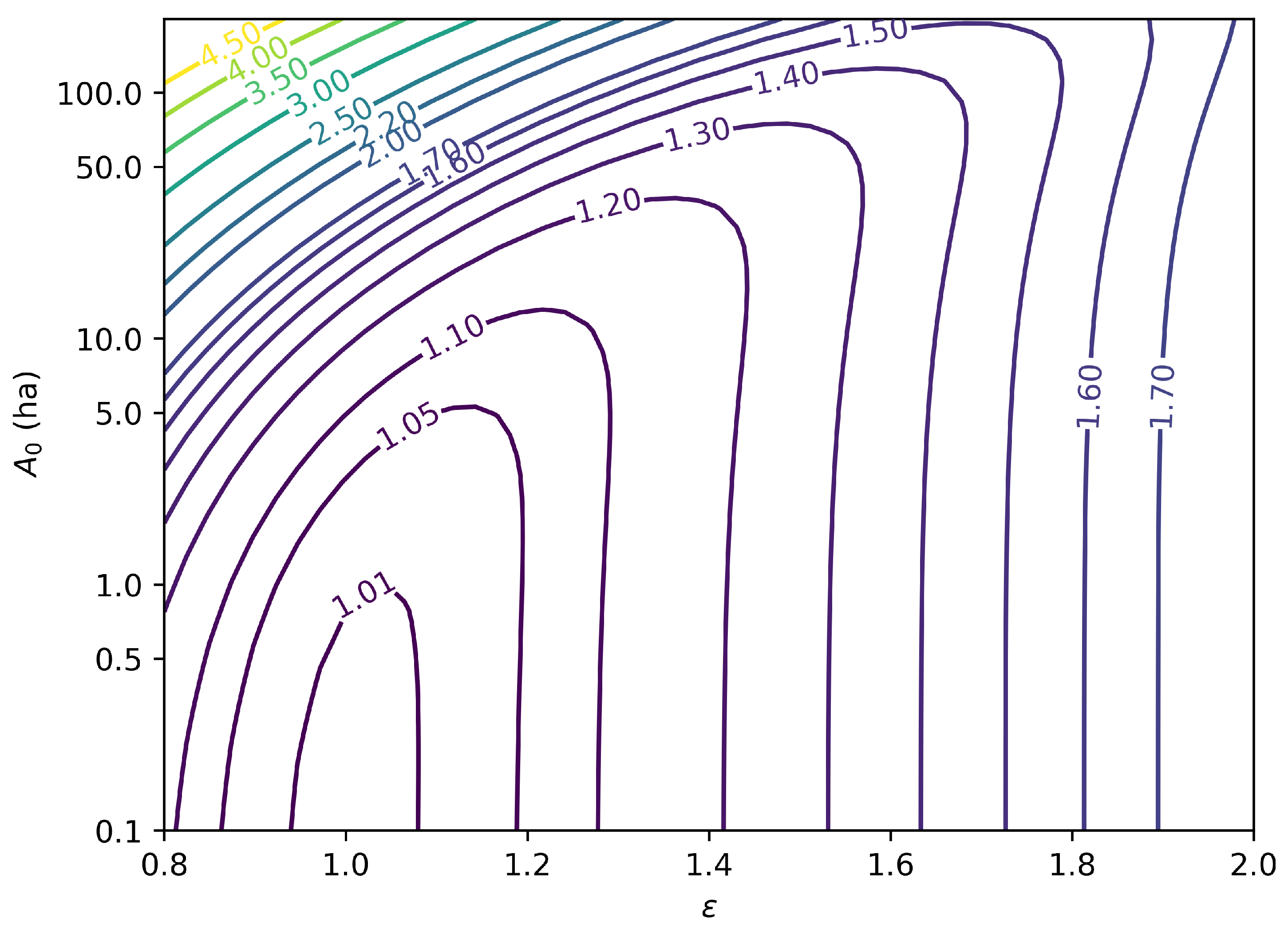
Figure 2.
Same-cost frequency multipliers for the optimal Importance Sampling scheme that reweights each pyrome uniformly. The color bar is logarithmic, and saturates to blue at 0.4 and to red at 2.5. More details in Table 2.
Figure 2.
Same-cost frequency multipliers for the optimal Importance Sampling scheme that reweights each pyrome uniformly. The color bar is logarithmic, and saturates to blue at 0.4 and to red at 2.5. More details in Table 2.
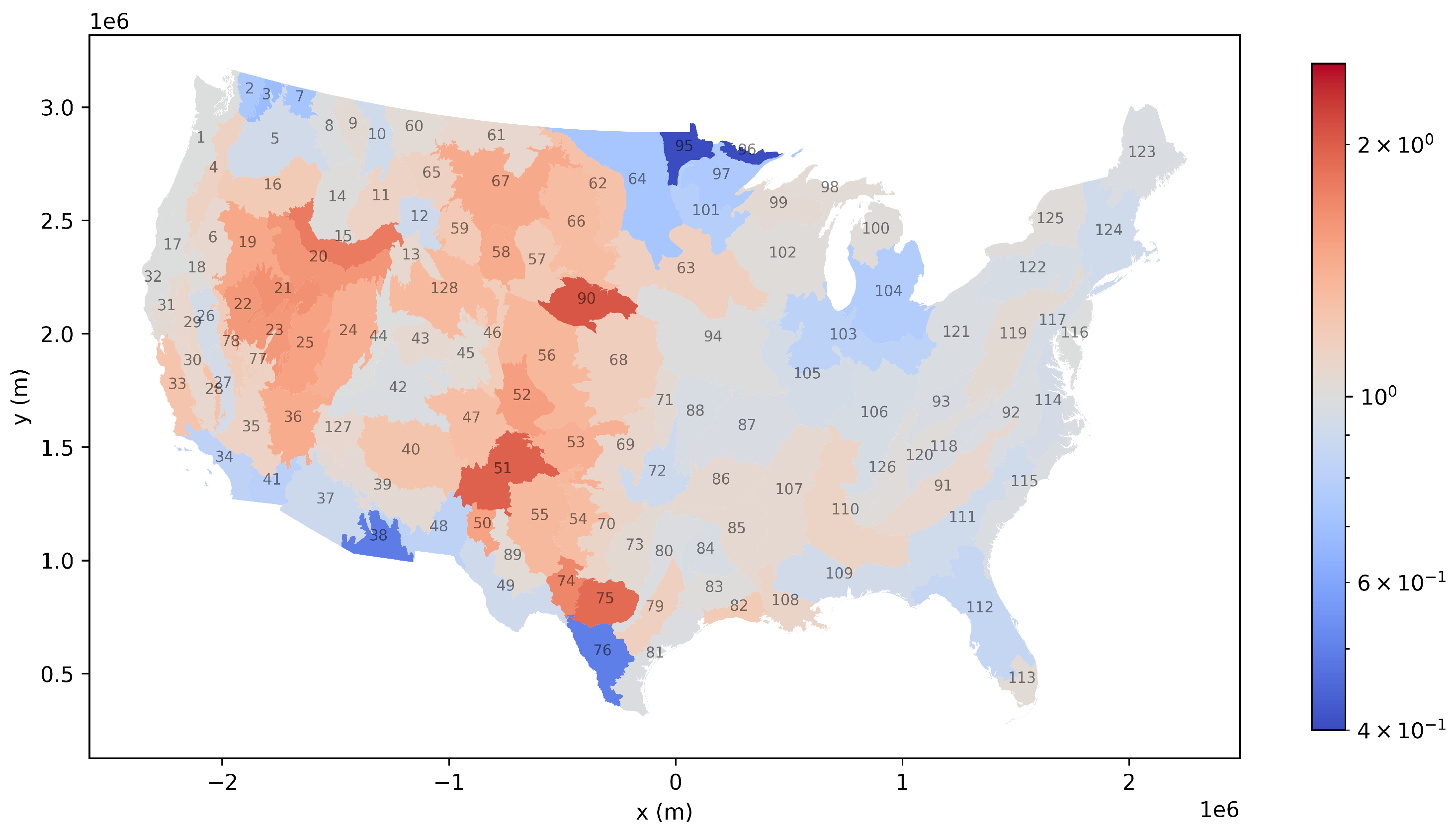
Figure 3.
Same-cost frequency multipliers for the reweighting function fitted to Pyrome 33 (solid curve), along with the best possible reweighting function (point cloud) of the calibration sample. means: for the same compute time, Importance Sampling multiplies by y the sampling frequency of a fire of duration x.
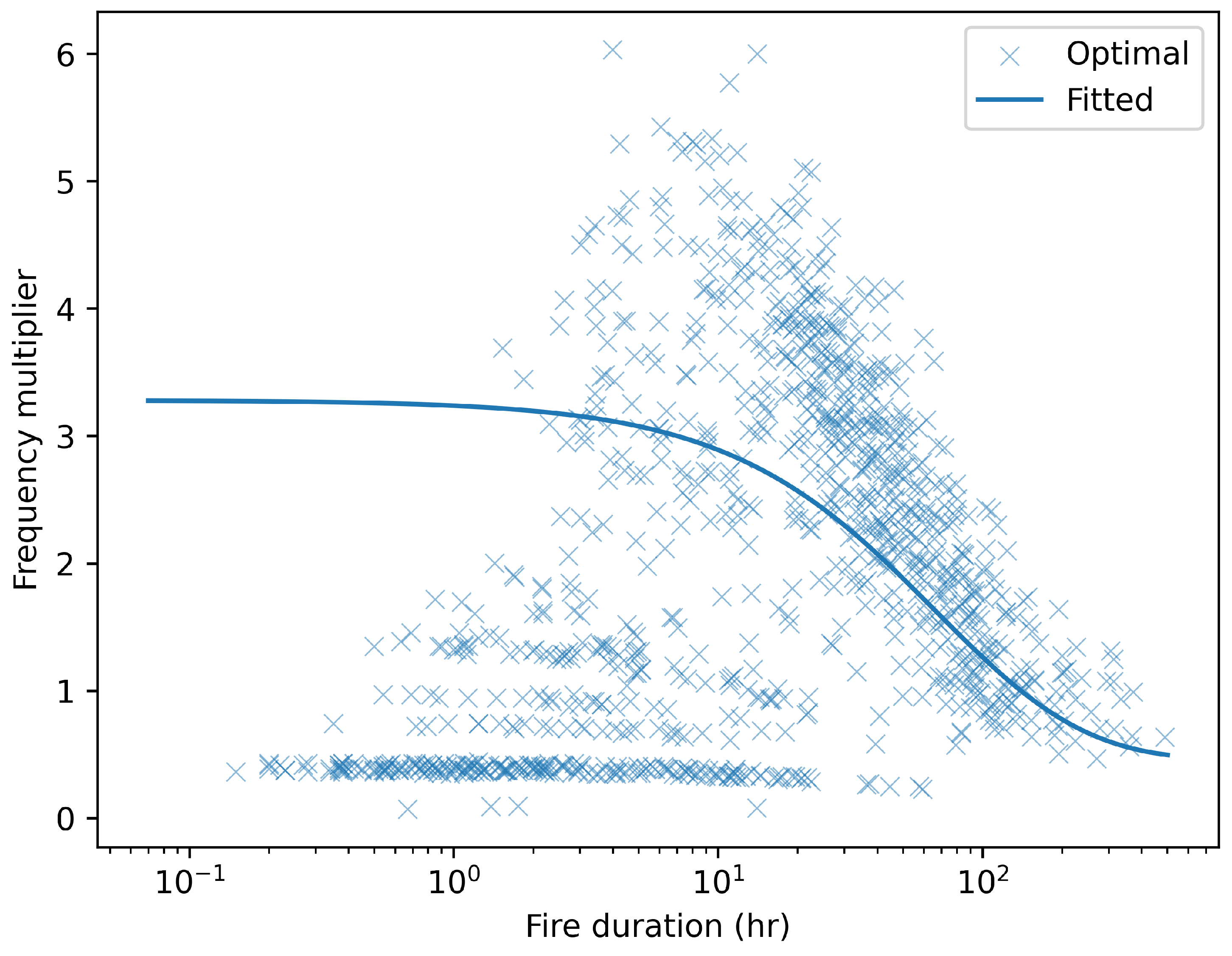
Figure 4.
Same-cost frequency multipliers for the reweighting function fitted to Pyrome 33 (solid curve), along with the best possible reweighting function (point cloud) of the calibration sample.
Figure 4.
Same-cost frequency multipliers for the reweighting function fitted to Pyrome 33 (solid curve), along with the best possible reweighting function (point cloud) of the calibration sample.
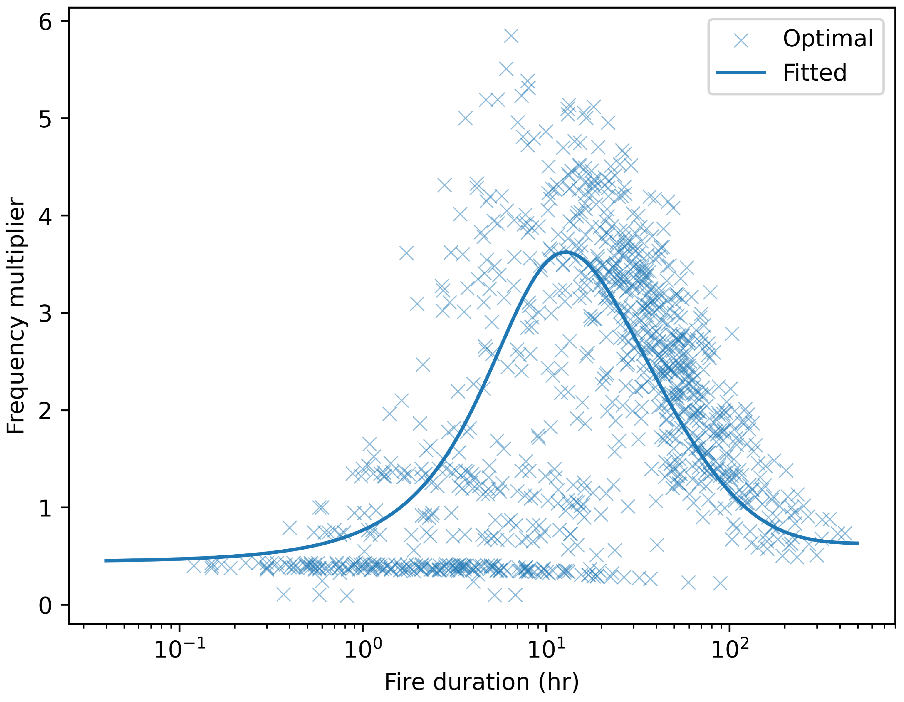

Table 1.
Table of Symbols
| Symbol | Type | Meaning |
|---|---|---|
| Same as | Expected value of random1 variable | |
| Variance of | ||
| Precision (inverse variance) of | ||
| Area of Interest | ||
| s | Spatial location | |
| F | (Potentially) simulated fire | |
| Random variable representing the natural distribution of simulated fires () | ||
| Area (or value) burned by fire F | ||
| Binary burn map (locations burned by F) | ||
| computational cost | ||
| Asymptotic burn-probability map (estimation target) | ||
| norm of map | ||
| impact-weighted norm of map | ||
| spatial density of (asset) value | ||
| Ignition or initial conditions | ||
| probability density of the natural distribution | ||
| probability density of a proposal distribution | ||
| Importance weight (ratio ) under proposal distribution q | ||
| Random variable representing the proposal distribution () | ||
| Importance Sampling estimator with proposal distribution q | ||
| Cost-to-precision ratio (inverse efficiency) | ||
| Efficiency gain: | ||
| optimal proposal distribution |
1Variables with a hat (like ) are subject to Monte Carlo randomness. 2 denotes the set of functions from set to set .
Table 2.
Fire statistics and same-cost frequency multipliers for the optimal Importance Sampling scheme that reweights each pyrome uniformly. The rightmost columns are expected values per simulated year. If a given pyrome has a multiplier of 1.3, it means that for the same amount of total compute time fires will be sampled 1.3 times more frequently from this pyrome under Importance Sampling than originally. In other words, if the original sampling procedure simulated 10,000 fire seasons in that pyrome, Importance Sampling now samples 13,000 fire seasons.
| Pyrome | Frequency multiplier | Model-predicted expected total | ||
| ID | (Same cost) | Burned area (ha/yr) | Runtime (s/yr) | Fires () |
| 1 | 1.00 | 4191.2 | 21.97 | 50.7 |
| 2 | 0.74 | 1509.5 | 14.17 | 19.6 |
| 3 | 0.68 | 16112.7 | 181.65 | 26.1 |
| 4 | 1.14 | 6427.3 | 25.61 | 51.9 |
| 5 | 0.92 | 58477.0 | 359.71 | 98.5 |
| 6 | 1.07 | 19684.2 | 88.78 | 19.0 |
| 7 | 0.72 | 32253.7 | 323.36 | 30.9 |
| 8 | 0.99 | 13646.9 | 73.00 | 22.6 |
| 9 | 1.04 | 20200.9 | 96.46 | 19.9 |
| 10 | 0.92 | 18636.2 | 115.63 | 23.7 |
| 11 | 1.13 | 28773.0 | 118.23 | 26.1 |
| 12 | 0.91 | 5986.2 | 38.03 | 9.6 |
| 13 | 1.07 | 6355.7 | 29.07 | 8.6 |
| 14 | 1.01 | 93709.1 | 477.19 | 107.5 |
| 15 | 1.79 | 77990.2 | 126.73 | 86.8 |
| 16 | 1.20 | 83122.4 | 300.23 | 73.4 |
| 17 | 0.99 | 42864.7 | 226.30 | 38.0 |
| 18 | 1.02 | 7899.4 | 39.51 | 3.6 |
| 19 | 1.47 | 29049.8 | 69.55 | 28.0 |
| 20 | 1.61 | 102857.4 | 206.72 | 70.5 |
| Pyrome | Frequency multiplier | Model-predicted expected total | ||
| ID | (Same cost) | Burned area (ha/yr) | Runtime (s/yr) | Fires () |
| 21 | 1.64 | 79368.3 | 153.83 | 28.9 |
| 22 | 1.59 | 7315.9 | 15.07 | 4.0 |
| 23 | 1.59 | 22119.1 | 45.65 | 4.5 |
| 24 | 1.41 | 57912.5 | 151.65 | 19.6 |
| 25 | 1.52 | 22139.9 | 50.08 | 3.8 |
| 26 | 0.93 | 20068.7 | 119.89 | 12.7 |
| 27 | 0.94 | 8690.8 | 50.76 | 5.5 |
| 28 | 1.27 | 20809.8 | 67.36 | 8.1 |
| 29 | 1.10 | 25451.7 | 109.37 | 15.3 |
| 30 | 1.08 | 21434.3 | 95.46 | 40.3 |
| 31 | 1.05 | 34229.6 | 161.90 | 26.2 |
| 32 | 1.00 | 14104.7 | 73.13 | 16.1 |
| 33 | 1.26 | 26953.8 | 88.63 | 31.5 |
| 34 | 0.82 | 69841.7 | 537.65 | 66.1 |
| 35 | 1.12 | 3954.4 | 16.28 | 4.7 |
| 36 | 1.45 | 23479.8 | 58.22 | 9.1 |
| 37 | 0.89 | 20517.2 | 133.50 | 30.9 |
| 38 | 0.49 | 26340.3 | 569.67 | 19.0 |
| 39 | 1.05 | 104106.2 | 490.07 | 14.9 |
| 40 | 1.26 | 6612.4 | 21.79 | 2.8 |
| 41 | 0.81 | 1688.9 | 13.52 | 3.4 |
| 42 | 0.97 | 12563.8 | 68.93 | 7.9 |
| 43 | 1.07 | 11667.0 | 53.55 | 7.8 |
| 44 | 1.00 | 22069.4 | 115.37 | 14.8 |
| 45 | 1.04 | 7342.0 | 35.48 | 7.4 |
| 46 | 1.18 | 27092.5 | 100.58 | 9.7 |
| 47 | 1.31 | 21751.2 | 66.38 | 4.2 |
| 48 | 0.82 | 4397.1 | 34.08 | 3.7 |
| 49 | 0.91 | 21746.4 | 136.82 | 12.6 |
| 50 | 1.52 | 13686.4 | 30.77 | 5.2 |
| 51 | 1.98 | 14818.8 | 19.67 | 5.7 |
| 52 | 1.54 | 5911.9 | 13.02 | 2.8 |
| 53 | 1.41 | 50181.2 | 131.02 | 23.7 |
| 54 | 1.32 | 23050.1 | 69.03 | 12.9 |
| 55 | 1.34 | 45158.7 | 130.02 | 48.8 |
| 56 | 1.36 | 9767.5 | 27.46 | 11.8 |
| 57 | 1.21 | 21448.6 | 75.86 | 11.9 |
| 58 | 1.45 | 8336.1 | 20.74 | 4.9 |
| 59 | 1.21 | 12332.9 | 43.69 | 9.3 |
| 60 | 1.04 | 5640.0 | 27.25 | 6.9 |
| 61 | 1.08 | 11456.3 | 51.21 | 14.2 |
| 62 | 1.28 | 1152.2 | 3.67 | 3.2 |
| 63 | 1.15 | 1894.4 | 7.40 | 25.2 |
| 64 | 0.73 | 5974.9 | 58.92 | 53.3 |
| 65 | 1.14 | 7788.4 | 31.15 | 4.4 |
| 66 | 1.32 | 18366.4 | 54.87 | 13.2 |
| 67 | 1.47 | 54847.9 | 132.00 | 35.1 |
| 68 | 1.17 | 9244.3 | 35.42 | 15.6 |
| 69 | 1.08 | 17408.7 | 77.19 | 17.9 |
| 70 | 1.11 | 22850.1 | 96.64 | 21.1 |
| 71 | 1.06 | 13200.3 | 61.42 | 9.4 |
| 72 | 0.90 | 35760.5 | 227.94 | 60.4 |
| 73 | 1.05 | 20397.4 | 97.16 | 15.7 |
| 74 | 1.72 | 11097.9 | 19.48 | 6.2 |
| 75 | 1.91 | 8693.3 | 12.47 | 6.3 |
| 76 | 0.50 | 7261.7 | 151.96 | 18.0 |
| 77 | 1.13 | 49.6 | 0.20 | 0.0 |
| 78 | 1.17 | 6659.3 | 25.22 | 4.2 |
| 79 | 1.16 | 2682.5 | 10.45 | 6.8 |
| 80 | 0.98 | 7371.4 | 39.82 | 16.5 |
| Pyrome | Frequency multiplier | Model-predicted expected total | ||
| ID | (Same cost) | Burned area (ha/yr) | Runtime (s/yr) | Fires () |
| 81 | 0.98 | 6986.1 | 37.50 | 42.5 |
| 82 | 1.20 | 10818.0 | 39.03 | 26.2 |
| 83 | 1.01 | 6063.0 | 30.89 | 48.5 |
| 84 | 0.96 | 3881.1 | 21.79 | 20.7 |
| 85 | 1.06 | 5546.6 | 25.64 | 45.9 |
| 86 | 1.06 | 12495.0 | 57.82 | 79.6 |
| 87 | 0.97 | 13980.1 | 77.81 | 67.5 |
| 88 | 0.96 | 6212.0 | 34.99 | 21.8 |
| 89 | 1.04 | 11715.3 | 56.52 | 14.3 |
| 90 | 2.06 | 5425.1 | 6.67 | 2.3 |
| 91 | 1.08 | 3879.9 | 17.43 | 65.4 |
| 92 | 0.97 | 2469.0 | 13.58 | 34.5 |
| 93 | 0.97 | 16873.5 | 93.54 | 627.9 |
| 94 | 1.00 | 3696.6 | 19.13 | 46.7 |
| 95 | 0.40 | 14253.1 | 475.06 | 69.9 |
| 96 | 0.39 | 1101.0 | 38.10 | 2.1 |
| 97 | 0.75 | 7047.1 | 65.41 | 65.5 |
| 98 | 1.04 | 964.2 | 4.67 | 20.5 |
| 99 | 1.06 | 680.5 | 3.18 | 14.5 |
| 100 | 1.02 | 1316.2 | 6.58 | 15.7 |
| 101 | 0.79 | 793.6 | 6.69 | 7.7 |
| 102 | 1.02 | 544.3 | 2.73 | 15.7 |
| 103 | 0.81 | 107.8 | 0.85 | 10.1 |
| 104 | 0.77 | 130.7 | 1.15 | 10.0 |
| 105 | 0.94 | 146.1 | 0.87 | 5.4 |
| 106 | 0.95 | 4321.1 | 24.81 | 91.9 |
| 107 | 1.06 | 2006.8 | 9.22 | 22.8 |
| 108 | 1.11 | 141.3 | 0.60 | 2.0 |
| 109 | 0.92 | 21235.4 | 130.98 | 137.4 |
| 110 | 1.11 | 8691.4 | 36.47 | 103.1 |
| 111 | 0.91 | 13278.6 | 83.02 | 114.6 |
| 112 | 0.86 | 57716.8 | 409.04 | 313.4 |
| 113 | 1.04 | 52045.2 | 252.31 | 45.0 |
| 114 | 0.94 | 1905.3 | 11.24 | 24.4 |
| 115 | 0.98 | 15348.7 | 84.02 | 123.8 |
| 116 | 1.00 | 2356.0 | 12.37 | 23.7 |
| 117 | 0.95 | 1816.4 | 10.42 | 14.0 |
| 118 | 0.97 | 3994.9 | 22.06 | 80.9 |
| 119 | 1.04 | 3806.6 | 18.19 | 26.6 |
| 120 | 1.02 | 11617.3 | 58.66 | 174.3 |
| 121 | 0.98 | 8300.3 | 45.44 | 199.3 |
| 122 | 0.96 | 1127.7 | 6.42 | 21.4 |
| 123 | 0.98 | 236.2 | 1.29 | 5.4 |
| 124 | 0.91 | 916.8 | 5.75 | 18.3 |
| 125 | 1.02 | 309.1 | 1.56 | 9.9 |
| 126 | 1.01 | 6965.1 | 35.50 | 152.1 |
| 127 | 1.08 | 12631.8 | 56.76 | 3.8 |
| 128 | 1.34 | 11486.8 | 33.47 | 11.8 |
Table 3.
Performance metrics of gradient-boosted tree models fitted to the example dataset. See text for details.
Table 3.
Performance metrics of gradient-boosted tree models fitted to the example dataset. See text for details.
| Model | Efficiency gain |
|---|---|
| Model A | 1.25 () |
| Model B | 1.15 () |
Disclaimer/Publisher’s Note: The statements, opinions and data contained in all publications are solely those of the individual author(s) and contributor(s) and not of MDPI and/or the editor(s). MDPI and/or the editor(s) disclaim responsibility for any injury to people or property resulting from any ideas, methods, instructions or products referred to in the content. |
© 2024 by the authors. Licensee MDPI, Basel, Switzerland. This article is an open access article distributed under the terms and conditions of the Creative Commons Attribution (CC BY) license (http://creativecommons.org/licenses/by/4.0/).
Copyright: This open access article is published under a Creative Commons CC BY 4.0 license, which permit the free download, distribution, and reuse, provided that the author and preprint are cited in any reuse.


