
Submitted:
10 October 2024
Posted:
11 October 2024
You are already at the latest version
Abstract
One of the most important aspects in the fabrication of car seats is the quality of its welded joints. In this proposal, a design of experiments (DoE) approach is used to improve the actual process capability (Cpk) of weld penetration depth in automotive seat adjusters using a laser beam welding (LBW) machine TRUMPF TruDiode 3006. Welding speed effects, laser power, and focal position in the Z axis were considered to determine the optimal welding penetration depth conditions, which is a minimum of 1.20 mm in cold rolled steel metal sheets ZE 790 with a thickness of 1.60 mm. The initial process capability evaluation indicated a Cpk value of 0.50, considering the initial process parameters. The proposed design was modeled using the response surface methodology, stepwise reduction technique, F-test, and before and after process capability evaluation for validation purposes. After applying the proposed methodology, a Cpk of 1.81 was obtained, resulting in a significant improvement of the process, reducing defective parts from 6.51% to 0.00%.
Keywords:
process capability
; laser beam welding
; design of experiments
; quality improvement
1. Introduction
Safety in the design of automotive structures is of utmost importance, especially in the design and manufacturing stages [1]. Seat structures engineers have faced a wide range of challenges when considering manufacturing and cost savings, which has influenced the improvement of design techniques. A car seat should be designed for the comfort of the passenger and to protect them from situations involving safety issues. The seat structure requires a simple, lightweight design to minimize material and manufacturing process costs. Despite the importance of seating structure design, many organizations are lack of resources to perform in-depth optimization analyses of multiple scenarios [1].
In the manufacturing processes of automotive seat structures, regulatory requirements must be met regarding the safety and quality of welding processes with metallic components or structural elements manufactured in production facilities. In this sense, [2] describes the importance of standards such as ISO 3834-1 (Quality requirements for fusion welding of materials), in [3]; ISO 14731 (Welding coordination. Tasks and responsibilities) in [4]; and EN 1090-2 (Execution of steel and aluminum structures. Part 2: technical requirements for the execution of steel structures) in [5], which include requirements for LBW processes.
LBW technology is increasingly being used in industrial applications not only for technical advantages in terms of material and product properties but also for benefits in terms of performance, production, and manufacturing capacity [6]. The design and manufacturing of small parts take advantage of technical processing innovations and economies of scale; in this type of application, LBW plays an important role in quality and safety aspects. LBW is a high-energy density beam welding process that is considered an alternative to conventional arc welding methods [7].
Among the advantages offered by this technology is the possibility of achieving welded joints at a high welding speed and with low heat input, which translates into high productivity, contributing to the process optimization and the reduction of manufacturing production costs [8].
Due to increasingly stringent technical and government requirements, manufacturing companies in the automotive industry face upward challenges in achieving lightweight structures, as well as complying with legal regulations to fulfill customer requirements.
Therefore, adequate welding processes are required, as well as operating with optimal parameters that allow all specifications to be met. That at the same time satisfies the, quality, and productivity to maintain competitiveness in the market [9].
Primarily, LBW takes advantage of three main factors: non-contact joining, single-sided joining technology, and a high-power beam capable of creating a welded joint in a fraction of a second [10]. LBW is a welding technology very suitable for the manufacturing of automotive structures. The LBW process requires a laser optical device installed on a robot and a scanning mirror head as the final reflector. An LBW machine can easily produce welded joints at different locations on a product by simply repositioning the robot or redirecting the laser beam via remote instructions.
An important aspect of the manufacturing process of automotive seat structures is the weld penetration depth that must be obtained when welding certain joints. The laser energy required for penetration depth using an LBW machine is small, approximately 1 mm/kW. On the other hand, the laser power can be modified during the welding process for application in different geometries. Joints in laser welding applications are heat transfer or keyhole type; likewise, the shape of the molten material depends on the welding speed, laser power, and focal position [11].
The choice to use keyhole-type laser welding occurs with power requirements greater than 106 W/cm2 due to its greater metal vaporization. Intense vaporization distinguishes keyhole laser welding from other welding processes because it causes a significant increase in vapor pressure (back pressure), which creates a narrow cavity or keyhole in the molten material. The laser beam can then penetrate deep into the metal through the cavity, refracting and damping as it travels through the vapor. When the laser beam reaches the surface of the cavity, the beam energy is partially absorbed at the surface and partially reflected to a new interaction point, creating the joint [12,13]. In this sense, in [14] a mathematical simulation approach of the temperature distribution and experimentation in the LBW is used to experimentally and numerically study the effect of each parameter.
An important aspect regarding welding manufacturing processes is the environmental impact, since, due to issues related to the design of the process, the equipment used and in general the manufacturing process itself, the raw materials used are not fully utilized [15]. In addition, to the generation of gases polluting the environment, especially those processes with high energy content. As with all welding processes, destructive testing is required to ensure the quality and reliability of the welded joint. A destructive test consists of microscopic measurements of a cross-section of a sample (specimen), to evaluate the weld penetration depth and determine whether the lot is accepted or rejected. Since it is not feasible to test 100% of each batch, a probability to reject an entire batch exists.
For welding processes, small production batches minimize the probability cost of rejecting an entire batch of material if a problem is found, but the cost per inspection and lead time for machine release are affected. In contrast, increasing the material lot size minimizes inspection cost and maximizes machine utilization, since the machine cannot begin production until the quality of the welded joints is verified. However, when a problem, such as a lack of weld penetration depth is detected during material inspection, the entire batch must be rejected, making reliable and robust process capability imperative. Therefore, the concept of sustainability has received special attention and support, as it provides a more holistic approach to the development and evaluation of welding processes [15].
In the literature, it is observed that interest has increased in how environmental improvements can be achieved through operational practices. In [16] describes the relationship between lean and problem-solving practices with reducing the environmental impact of an organization. The green management approach contributes to cost reduction by using resources such as raw materials more efficiently, which also positively influences the organization’s results [17].
Therefore, the main challenges for industrial organizations such as the automotive welding industry, in terms of sustainability and competitiveness, are linked to defect-free products, and fast, efficient, flexible, but also environmentally friendly manufacturing processes [18].
Increased competition in many industries is accompanied by increasing cost pressure. This poses the frequent challenge of identifying and optimizing new and/or improved value-added processes [19]. Process capability assessment can effectively address the statistical performance of the process with a dimensionless indicator. Potential process capability (Cp) and actual process capability (Cpk) are statistical measures that quantify process variation, equivalent to plus/minus three standard deviations (σ) from the mean for comparison with the specification tolerance. (Customer requirements) [20]. These indices are effective tools for both process capability analysis and quality assurance. Understanding process variation and evaluating process performance are essential tasks in quality improvement projects [20].
As stated in [20], the actual process capability index Cpk should be considered for the initial evaluation of critical customer characteristics to determine the capability of the process to meet those requirements. During the production process, statistical evaluation of process control is needed to monitor process stability and randomness of process behavior before evaluating process capability [20]. It is necessary to meet assumptions of normality and stability before making inferences about the capacity of the process [21,25].
Capability analysis can help decision-makers better understand the process and thus achieve important quality improvements [22]. From a quality perspective, the Cpk is expected to be greater than or equal to 1.33. Therefore, a Cpk less than 1.00 is evidence that the process cannot meet specifications [21,23,25,26].
Table 1 summarizes different approaches for similar performed weld penetration depth studies found in the literature using LBW technology, as well as the contribution of this proposal. These contributions range from destructive testing and theoretical-empirical analysis [27], to artificial neural networks and finite element analysis [4,28]. In [7,29,30,31,32], the Design of Experiments (DoE) methodology for analysis was applied.
In this paper, the case of a low level of weld penetration depth is addressed, which must be greater than or equal to 1.2 mm for T-type joints between a side panel and the upper rail which are joined to integrate a car seat structure by fusion welding. Through the PDCA (plan-do-check-act) cycle methodology, an evaluation of the capability of the current process is carried out to determine the necessary improvements: change the mean, reduce the process variation, or do both [21,33]. Subsequently, the DoE Response Surface Methodology (RSM) is used as a tool to characterizes the factors that influence the output variable (y), to determine the optimal process parameters. Finally, a confirmation test of process capacity is conducted to validate and quantify the improvements achieved.
The rest of the paper is organized as follows: Section II present the case of study, describes the PDCA cycle improvement model and the response surface model (RSM) approach. Section III presents the results of the case study. Section IV discussion about the optimized model. Finally, in section V the conclusions achieved in the long term are presented.
2. Case of Study
When deciding which technological welding process should be defined: the material to be welded, the geometry of the seam weld and the welding type, and subsequently the process parameters, mainly the laser power, the welding speed, and the focal position [11]. ZE 790 cold rolled steel was used in this case of study due to the low carbon equivalent concentration (CE): CE = 0.182. The chemical composition of the material under study is described in Table 2. This type of steel is ideal for laser welding applications, with no decrease in the elastic limit being observed in the areas affected by heat. Furthermore, the high ratio between yield strength and tensile strength provides excellent preconditions for a roll-forming process [38]. The yield strength of ZE 790 steel is 800 MPa.
2.1. Output Variable – Measurable (y) Definition
For T-type joints, the output variable (y), i.e., weld penetration depth, is defined as the minimum distance that the fusion line extends to the root between the two metal plates [34], as shown in Figure 1.
The measurement variable (y) was evaluated using a Leica M80III optical microscope. Figure 2 shows a cut and polished macrograph of a rejected specimen at the current stage. As shown, a weld penetration depth is less than the minimum of 1.20 mm specification, which established the baseline of the case study presented. Samples were prepared metallographically prepared using a conventional technique according to ASTM E3, then etched with a combination of four-step sanding and polishing process using 80 grits (coarse) SiC sandpaper up to 2400 grit for smoothing, a combination of methanol and nitric acid was used as a developer to visualize the microstructure.
2.2. PDCA Cycle Methodology
The PDCA improvement cycle is a well-known methodology for addressing quality improvement initiatives [21,33]. Figure 3 describes the application of the PDCA framework in the case of study.
In the proposed PDCA conceptual framework, a baseline process capability evaluation was carried out with 25 historical data readings of the solder joint under analysis. The sample size was determined to produce no violations of normality assumptions and to have a reasonable margin of error of 0.0126 for the mean estimate. In addition, batch-to-batch and time-to-time variation in the analyzed data was considered to meet the sampling criteria, as discussed in [21,35,36].
Initial process capability assessment indicates that the Cpk statistic of the current process is 0.50, which establishes that this process is unable to achieve a minimum weld penetration depth of 1.2 mm. Figure 4 shows the process capacity analysis obtained through the Minitab™ 21 statistical software [37].
2.3. Design of Experiments – RSM Approach
To carry out the DoE process, a TRUMPF TruDiode 3006 laser machine was used, with a power of 3 kW and a 600 μm lens, under the keyhole regime. The components position (side panel and top rail) was controlled with pneumatic clamping devices. Table 3 summarizes the process parameters used by the DoE in this case study. Three factors (A—welding speed, B—laser power, and C—Z-axis focal position) were defined to determine the optimal conditions to improve the weld penetration depth, with a minimum requirement of 1.20 mm, for a cold rolled stamped steel subassembly with a thickness of 1.60 mm.
For the application of the DoE and the RSM methodology, a full 23 factorial design with a center point is used. RSM consists of a set of mathematical and statistical techniques useful for modeling and analyzing problems in which more than one variable influences a response of interest. The goal is to optimize this response. Therefore, the first step in RSM is to find a suitable approximation for the true functional relationship between (y) and the set of independent variables. If there is curvature in the system, a polynomial of higher degree must be used, such as the second-order model defined below [39]:
The coding factors for DoE, shown in Table 4, were confirmed with a visual check.
3. Results
Once the factors (A, B, and C) were coded, the orthogonal matrix was defined for a complete factorial design with three factors and two levels, that is, 23 DoE, giving eight possible combinations. Additionally, a treatment was added to evaluate the curvature with fixed values at the center point of the experimental window, as detailed in Table 5. Three repetitions were performed for each treatment (experiment), giving a total of (27-1) degrees of freedom for the analysis.
Table 6 describes the analysis of variance, (ANOVA). This estimation of effects, evaluates the significance of one or more factors by comparing the means of the response variable at different levels [40] of the experiment using RSM for the assessment. A stepwise technique was applied, adding terms to make the model hierarchical [39]; see Table A1 of the Appendix A for details. According to Table 6, the model is statistically significant with a probability value (P-value) of 0.000; furthermore, the ANOVA table shows the significant quadratic effect for speed and double interactions, all with (P-values) less than 0.05. The lack of fit test was also satisfactory, with a (P-value) greater than 0.05; a residual analysis confirmed the model’s predictability with no multicollinearity issues. See Figure A1 of the Appendix B.
As shown in the ANOVA table, the linear effects of laser power and focal position affect welding penetration [7,27,30,31] in the automotive seat structure seam weld under study with a significance level of 0.05, so the null hypothesis is rejected [39,40]. With a total of 26 degrees of freedom, the model meets the sample size needed to perform an analysis of the quadratic effects and the double interaction effects from the DoE main factors, as summarized in the ANOVA table:
- • Quadratic effect of Speed (AA),
- • Double interactions of Speed-Power (AB) and Speed-Focal Position (AC)
Thanks to the stepwise technique, the remaining double interactions and non-significant quadratic effects are discarded with a confidence level of 95%.
Based on Table 6, the calculated F-value, which indicates the magnitude of the effect, for the focal position is 271.29, which shows the most significant impact on weld penetration [7], as shown in Figure 5.
Table 7 shows the coefficients of the regression equation; variance inflation analysis (VIF) was also performed, with no collinearity problems observed, VIF = 1.00 [39]. The coefficient of determination R-sq = 94.64% and R-sq (pred) = 90.46% were obtained, indicating that the model is highly accurate for prediction. Furthermore, the laser speed coefficient has a (P-Value) of 0.087, which implies that this factor is not statistically significant at the 95.0% confidence level.
The regression equation obtained by the DoE stepwise experimentation technique using the RSM methodology is described as:
where y represents the response variable.
y = 1.2267 – 0.0367 A – 0.0725 B – 0.3358 C – 0.3925 A*A + 0.0467 A*B – 0.0900 A*C
4. Discussion
Figure 6 shows the graphic analysis of the behavior of the response variable (y) using (2). The red outline indicates a weld penetration depth for y < 1.20 mm. Areas with gray lines are below 1.00 mm, indicating "crack" regions; the light gray dashed area indicates a weld penetration depth greater than 1.60 mm, which causes a blow hole condition due to the material thickness of 1.60 mm; the yellow region is acceptable; and the green zone indicates an optimal and desirable region for weld penetration depth [32].
Figure 6a shows the relationship between welding speed and laser power when the focal position is set to 224.15 mm; Figure 6b shows the relationship between welding speed and focal position when the laser power is set to 2500 kW; Figure 6c shows the relationship between focal position and laser power when the welding speed is set to 30 mm/s. The desirable zone for measurable weld penetration depth (y), is between 1.20 and 1.40 mm, which is highlighted in green. The contour analysis allows the evaluation of different behavior of the response variable depending on how the process parameters are adjusted. Figure 6a and 6b show a quadratic relationship between the adjustment factors and the depth of penetration of the weld, while Figure 6c indicates a linear relationship between laser power and focal position versus weld penetration depth, justifying the use of RSM for the optimization of (y) [39].
After the first step in RSM, as shown in Figure 6, the weld penetration depth is sought to be set to y ≈ 1.35 mm. To optimize the response variable, Table 8 summarizes the proposed optimal process parameters. The welding speed was set to a nominal value of 30 mm/s, the laser power was set to a nominal value of 2500 kW, and the focal position was set to 224.02 mm to achieve the desirable weld penetration depth of 1.35 mm, which is optimal to avoid cracks or blow holes, as indicated in Figure 6.
The RSM using the stepwise technique shows significant statistical evidence of the main contributors that influence the weld penetration depth for automotive seat rails, which are: focal position (Z axis) and the quadratic effect of welding speed. This information indicates that the process parameters need to be adjusted the focal position from 224.15 to 224.02 mm. Furthermore, the welding speed range sett was reduced due to its quadratic effect on the output variable: from 28–38 to 28–32 mm/s, as shown in Figure 6. Finally, the DoE demonstrated that the Laser power should operate at the average level of 2500 kW, which contributes in the long term to optimizing energy consumption. Figure 7 shows a macrograph specimen using the process parameters indicated in Table 8.
Finally, a validation run was carried out considering the variation due to common causes, that is, different batches of materials and production shifts. Table 9 indicates the process capability index improved from Cpk = 0.50 to Cpk = 1.81, this means that the percentage of parts not meeting the required weld penetration depth was reduced from 65,086 parts per million (ppm) to 0 ppm. Figure 8 graphically depicts the mean change before and after the application of the PDCA framework for waste elimination and process capability improvement. Therefore, the performance optimization of the weld penetration depth process using the LBW machine can be established through RSM.
5. Conclusions
This paper proposes the use of the RSM methodology to establish a technical solution to the current problem of adjusting welding parameters in the automotive industry and other industries with similar applications when there is evidence that at least one of the factor analyses affects non-linear the response studied; demonstrating the robustness of this technique to satisfy Cpk requirements, so the following is established:
1. Using the regression equation obtained from DoE, the optimized parameters achieved a Cpk of 1.81 with an R-sq (pred) of 90.46%. Waste generated by failures in weld penetration depth (<1.20 mm) was reduced from 6.51% to 0.00%.
2. The depth of weld penetration in ZE 790 cold-rolled steel joints depends on the focal position of the welding beam, the welding speed, which provides a quadratic effect, and the applied laser power (energy).
3. Using RSM to understand weld penetration depth phenomena before and after response optimization and with a second-order regression (2) is a statistically sound approach to meet customer requirements and current welding standards for light products used in the automotive industry.
4. The methodology discussed in this article is part of a promising efficient and green approach to saving time and money. It involves performing in-depth analysis of multiple scenarios to optimize weld penetration depth, contribute to the sustainability of the welding process, dramatically reduce waste of non-conforming material, and enable more efficient utilization of equipment. As a result, the economic impact of the organization is positively affected.
Author Contributions
Conceptualization, J.T. and H.M.; methodology, H.M.; software, J.T.; validation, J.T., H.M. and A.M.; formal analysis, J.T.; investigation, J.T.; resources, J.T.; data curation, J.T.; writing—original draft preparation, J.T.; writing—review and editing, J.T., H.M., A.M. and O.M.; visualization, O.M.; supervision, H.M.; project administration, J.T.; funding acquisition, J.T. All authors have read and agreed to the published version of the manuscript.
Funding
This research received no external funding.
Data Availability Statement
Data availability upon request.
Acknowledgments
We would like to thank the entire troubleshooting team at the Brose Tuscaloosa, Alabama plant for their contribution to the development of the research studies, especially Jim Barbaretta for his support and sponsorship as former Plant Manager.
Conflicts of Interest
The authors declare no conflicts of interest.
Appendix A

Table A1.
Details of the stepwise technique4.
| ------Step 1----- | ------Step 2----- | ------Step 3----- | ||||||
| Term | Coef | P | Coef | P | Coef | P | ||
| Constant | 0.8778 | 1.2267 | 1.2267 | |||||
| C | −0.3358 | 0.000 | −0.3358 | 0.000 | −0.3358 | 0.000 | ||
| AA | −0.3925 | 0.000 | −0.3925 | 0.000 | ||||
| AC | −0.0900 | 0.003 | ||||||
| B | ||||||||
| AB | ||||||||
| A | ||||||||
| S | 0.201539 | 0.158723 | 0.133552 | |||||
| R-sq | 72.72% | 83.76% | 88.98% | |||||
| R-sq(adj) | 71.63% | 82.40% | 87.54% | |||||
| R-sq(pred) | 68.84% | 80.66% | 85.59% | |||||
| AICc | −4.91 | −16.13 | −23.57 | |||||
| BIC | −2.06 | −12.77 | −19.94 | |||||
| ------Step 4----- | ------Step 5----- | ------Step 6----- | ||||||
| Term | Coef | P | Coef | P | Coef | P | ||
| Constant | 1.2267 | 1.2267 | 1.2267 | |||||
| C | −0.3358 | 0.000 | −0.3358 | 0.000 | −0.3358 | 0.000 | ||
| AA | −0.3925 | 0.000 | −0.3925 | 0.000 | −0.3925 | 0.000 | ||
| AC | −0.0900 | 0.001 | −0.0900 | 0.000 | −0.0900 | 0.000 | ||
| B | −0.0725 | 0.005 | −0.0725 | 0.003 | −0.0725 | 0.002 | ||
| AB | 0.0467 | 0.041 | 0.0467 | 0.033 | ||||
| A | −0.0367 | 0.087 | ||||||
| S | 0.113635 | 0.105066 | 0.0998874 | |||||
| R-sq | 92.37% | 93.77% | 94.64% | |||||
| R-sq(adj) | 90.98% | 92.29% | 93.03% | |||||
| R-sq(pred) | 89.00% | 90.05% | 90.46% | |||||
| AICc | −30.14 | −31.94 | −31.88 | |||||
| BIC | −26.57 | −28.76 | −29.51 | |||||
4 Candidate terms: A, B, C, A*A, B*B, C*C, A*B, A*C, B*C; α to enter = 0.15; α to remove = 0.15.
Appendix B
Figure A1.
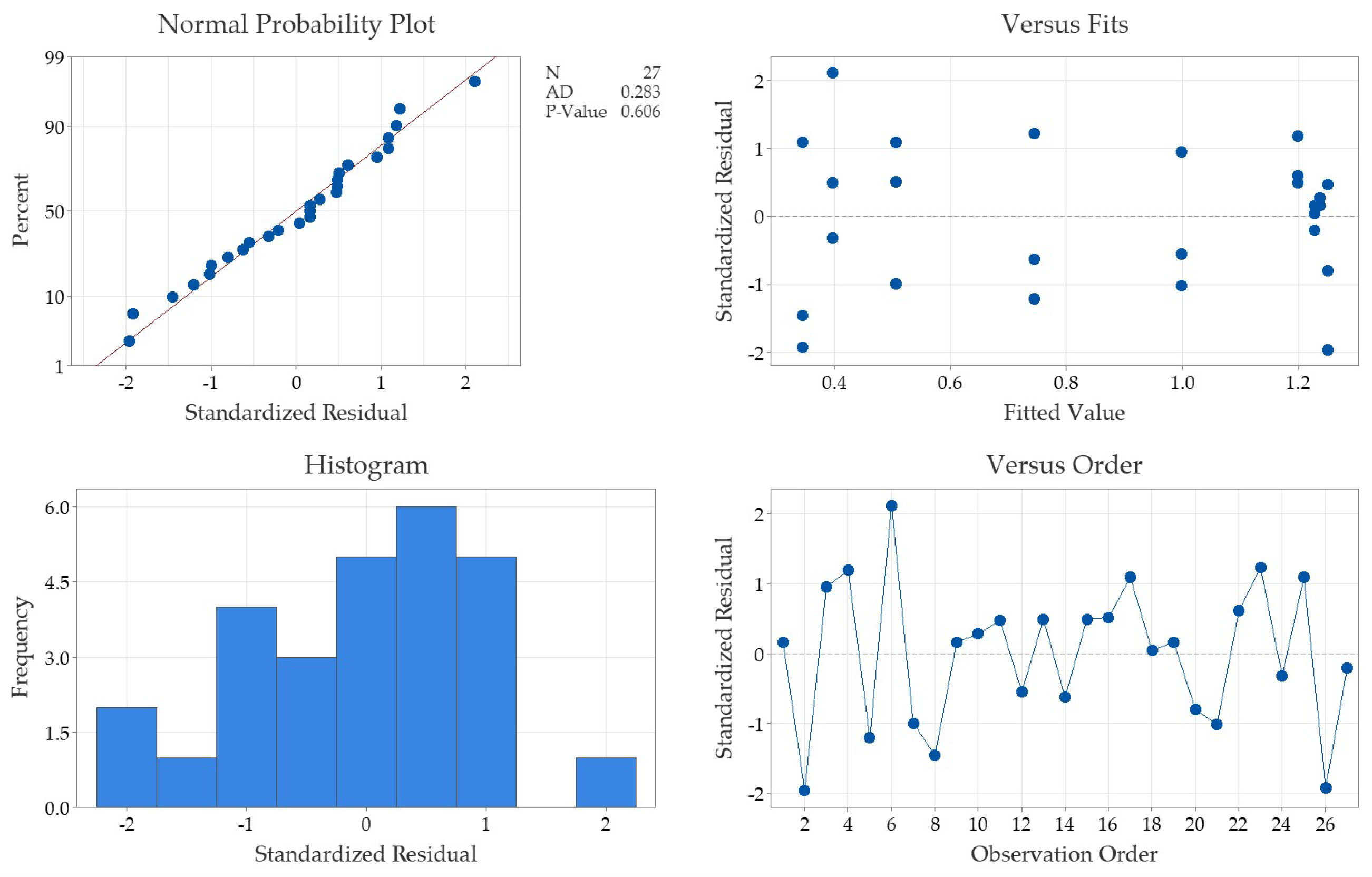
Residual plots for weld depth penetration y (mm) for the normality assessment.
References
- S. Jong-Kang, B. Kchunb, “An effective approach to prediction of the collapse mode in automotive seat structure”. Thin-Walled Structures, vol, 37 issue 2, pp. 113-125, 2000. [CrossRef]
- Manzanares-Cañizares, C.; Sánchez-Lite, A.; Rosales-Prieto, V.F.; Fuentes-Bargues, J.L.; González-Gaya, C. A 5S Lean Strategy for a Sustainable Welding Process. Sustainability 2022, 14, 6499. [CrossRef]
- ISO (International Organization for Standardization). ISO 3834-1; Quality Requirements for Fusion Welding of Metallic Materials – Part1: Criteria for selection of the appropriate level of quality requirements; 2021.
- ISO (International Organization for Standardization). ISO 14731; Welding coordination – Task and Responsibilities; 2019.
- EN (European Standard). EN 1090-2; Execution of Steel Structures – Part 2: Technical requirements for the execution of steel structures; 2018.
- Zhou, L.; Luo, L.; Tan, C.; Li, Z.; Song, X.; Zhao, H.; Huang, Y.; Feng, J.; Zhou, L.; Luo, L.; et al. Effect of welding speed on microstructural evolution and mechanical properties of laser welded-brazed Al/brass dissimilar joints. Opt. Laser Technol. 2018, 98, 234–246. [CrossRef]
- Madrid, J.; Lorin, S.; Söderberg, R.; Hammersberg, P.; Wärmefjord, K.; Lööf, J. A Virtual Design of Experiments Method to Evaluate the Effect of Design and Welding Parameters on Weld Quality in Aerospace Applications. Aerospace 2019, 6, 74. [CrossRef]
- Reddy, B.N.; Hema, P.; Vardhan, G.V.; Padmanabhan, G. Experimental Study of Laser Beam Welding Process Parameters on AISI 4130-309 Joint Strength. Mater. Today: Proc. 2020, 22, 2741–2750. [CrossRef]
- Schmoeller, M.; Stadter, C.; Wagner, M.; Zaeh, M.F. Investigation of the influences of the process parameters on the weld depth in laser beam welding of AA6082 using machine learning methods. Procedia CIRP 2020, 94, 702–707. [CrossRef]
- Ceglarek, D.; Colledani, M.; Váncza, J.; Kim, D.-Y.; Marine, C.; Kogel-Hollacher, M.; Mistry, A.; Bolognese, L. Rapid deployment of remote laser welding processes in automotive assembly systems. CIRP Ann. 2015, 64, 389–394. [CrossRef]
- Kovacs, T. Laser welding process specification base on welding theories. Procedia Manuf. 2018, 22, 147–153. [CrossRef]
- J. Svenungsson, I. Choquet; A.F.H. Kaplan, “Laser welding process – a review of keyhole welding modelling”, Physics Procedia, vol. 78, pp. 182-191, 2015. [CrossRef]
- D. Vieira, J.E. May, G.S. Savonov, R.H.M. Siqueira, M.S.F. Lima, “Determination of tensile shear strength and corrosion behavior of circular bead produced by a laser beam for overlapped AISI 304 steel sheets” Soldagem & Inspeção, vol. 26, e2614, 2021. [CrossRef]
- Chandelkar, V.; Pradhan, S.K. Numerical simulation of temperature distribution and experimentation in laser beam welding of SS317L alloy. Mater. Today: Proc. 2020, 27, 2758–2762. [CrossRef]
- Jamal, J.; Darras, B.; Kishawy, H. A study on sustainability assessment of welding processes. Proc. Inst. Mech. Eng. Part B: J. Eng. Manuf. 2019, 234, 501–512. [CrossRef]
- M. J. Alves-Pinto-Jr, J. Veiga-Mendes, “Operational Practices of Lean Manufacturing: Potentiating Environmental Improvements,” Journal of Industrial Engineering and Management, vol. 10, no. 4, pp. 550-580, 2017. [CrossRef]
- Azevedo, S.G.; Carvalho, H.; Duarte, S.; Cruz-Machado, V. Influence of Green and Lean Upstream Supply Chain Management Practices on Business Sustainability. IEEE Trans. Eng. Manag. 2012, 59, 753–765. [CrossRef]
- Dakov, I.; Novkov, S. Assessment of the Lean Production Effect on the Sustainable Industrial Enterprise Development. Business: Theory Pr. 2007, 8, 183–188. [CrossRef]
- Beske, P.; Koplin, J.; Seuring, S. The use of environmental and social standards by German first-tier suppliers of the Volkswagen AG. Corp. Soc. Responsib. Environ. Manag. 2006, 15, 63–75. [CrossRef]
- R. Raut, P. R. Attar, “Optimization of process capability in an automobile industry: A case study,” International Research Journal of Engineering and Technology, vol. 3, issue. 7, pp. 289-295, 2016.
- R. A. Munro, G. Ramu, D. J. Zrymiak, “The Certified Six Sigma Green Belt Handbook,” ASQ Quality Press, pp. 237-252, 2015.
- S. B. Amara, J. Dhahri, N. B. Fredj, “Process True Capability Evaluation with the Consideration of Measurement System Variability and Expected Quality Loss,” Quality Reliability Engineering International, vol. 33, p.p. 937-944, 2016. [CrossRef]
- Czarski, K. Satora, P. Matusiewicz, “Statistical Methods in Quality Management – Process Capability Analysis,” Metallurgy and Foundry Engineering, vol. 33, no. 2, pp. 121-128, 2007. [CrossRef]
- Dobránsky, J.; Pollák, M.; Doboš, Z. Assessment of Production Process Capability in the Serial Production of Components for the Automotive Industry. Manag. Syst. Prod. Eng. 2019, 27, 255–258. [CrossRef]
- Montgomery, D.C., Introduction to Statistical Quality Control. John Wiley & Sons, Inc. 2009.
- Prasad, S.; Bramorski, T. Robust process capability indices. Omega 1998, 26, 425–435. [CrossRef]
- Paes, L.E.d.S.; Pereira, M.; Weingaertner, W.L.; Scotti, A.; Souza, T. Comparison of methods to correlate input parameters with depth of penetration in LASER welding. Int. J. Adv. Manuf. Technol. 2018, 101, 1157–1169. [CrossRef]
- Pavlíček, K.; Kotlan, V.; Doležel, I. Estimation of laser weld parameters using surrogate modelling technique. J. Electr. Eng. 2018, 69, 170–176. [CrossRef]
- Khorram, A.; Ghoreishi, M.; Yazdi, M.R.S.; Moradi, M. Optimization of Bead Geometry in CO2 Laser Welding of Ti 6Al 4V Using Response Surface Methodology. Engineering 2011, 03, 708–712. [CrossRef]
- Yufeng, S.; Sili, F.; Changwei, X. Optimization of welding process of heterogeneous high strength steel based on PLC control. Results Phys. 2018, 11, 817–820. [CrossRef]
- G., K.K.; C., V.; T., K. Using the RSM method of improving process parameters of welding AISI 316 and nickel 201 using CO2 laser. Mater. De Jan. 2022, 27. [CrossRef]
- Khan, M.; Romoli, L.; Fiaschi, M.; Dini, G.; Sarri, F. Experimental design approach to the process parameter optimization for laser welding of martensitic stainless steels in a constrained overlap configuration. Opt. Laser Technol. 2011, 43, 158–172. [CrossRef]
- A. M. Munteanu, “Comparative Analysis between Lean, Six Sigma and Lean Six Sigma Concepts,” Management and Economics Review, vol. 2, issue, 1, 78-89, 2017.
- Mansour, R.; Zhu, J.; Edgren, M.; Barsoum, Z. A probabilistic model of weld penetration depth based on process parameters. Int. J. Adv. Manuf. Technol. 2019, 105, 499–514. [CrossRef]
- J. Uttley, “Power Analysis, Sample Size, and Assessment of Statistical Assumptions Improving the Evidential Value of Lighting Research,” The Journal of the Illuminating Engineering Society, vol. 15, issue. 2-3, pp. 143-162, 2019. [CrossRef]
- H. Ahmad, H. Halim, “Determining Sample Size for Research Activities,” The Case of Organizational Research, Selangor Business Review, pp. 20-34, 2017.
- Minitab® 21.1 (64-bit), Statistical Software. Available online: URL https://www.minitab.com/en-us/products/minitab/ (12/14/2023).
- Bilstein Coil Roled Steel. Bilstein ZE Grades. Available online: URL http://www.bilsteincrs.com/products/bilstein-ze-grades/ (10/30/2023).
- Montgomery, D.C., Design and analysis of experiments. John Wiley & Sons, Inc. 2017.
- Bharathikanna, R.; Elatharasan, G. Microstructure, Mechanical and Corrosion Behavior of Friction Stir Processed AA6082 with Cr3C2 Particles. Soldag. Inspecao 2022, 27. [CrossRef]
Figure 1.
Measurable (y) definition of weld penetration depth.
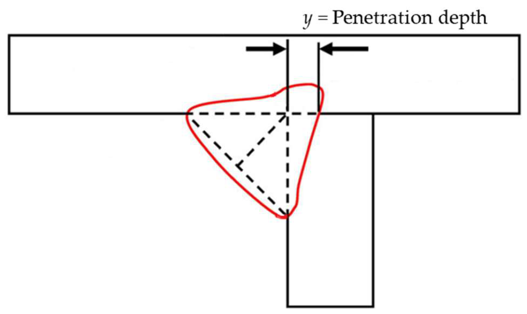
Figure 2.
Ground and polished macrograph of ZE 790 steel welded by LBW from a rejected specimen of weld penetration depth not fulfilling the specification (1.20 mm minimum), showing the (a) side panel, (b) upper rail, and (c) weld penetration depth.
Figure 2.
Ground and polished macrograph of ZE 790 steel welded by LBW from a rejected specimen of weld penetration depth not fulfilling the specification (1.20 mm minimum), showing the (a) side panel, (b) upper rail, and (c) weld penetration depth.
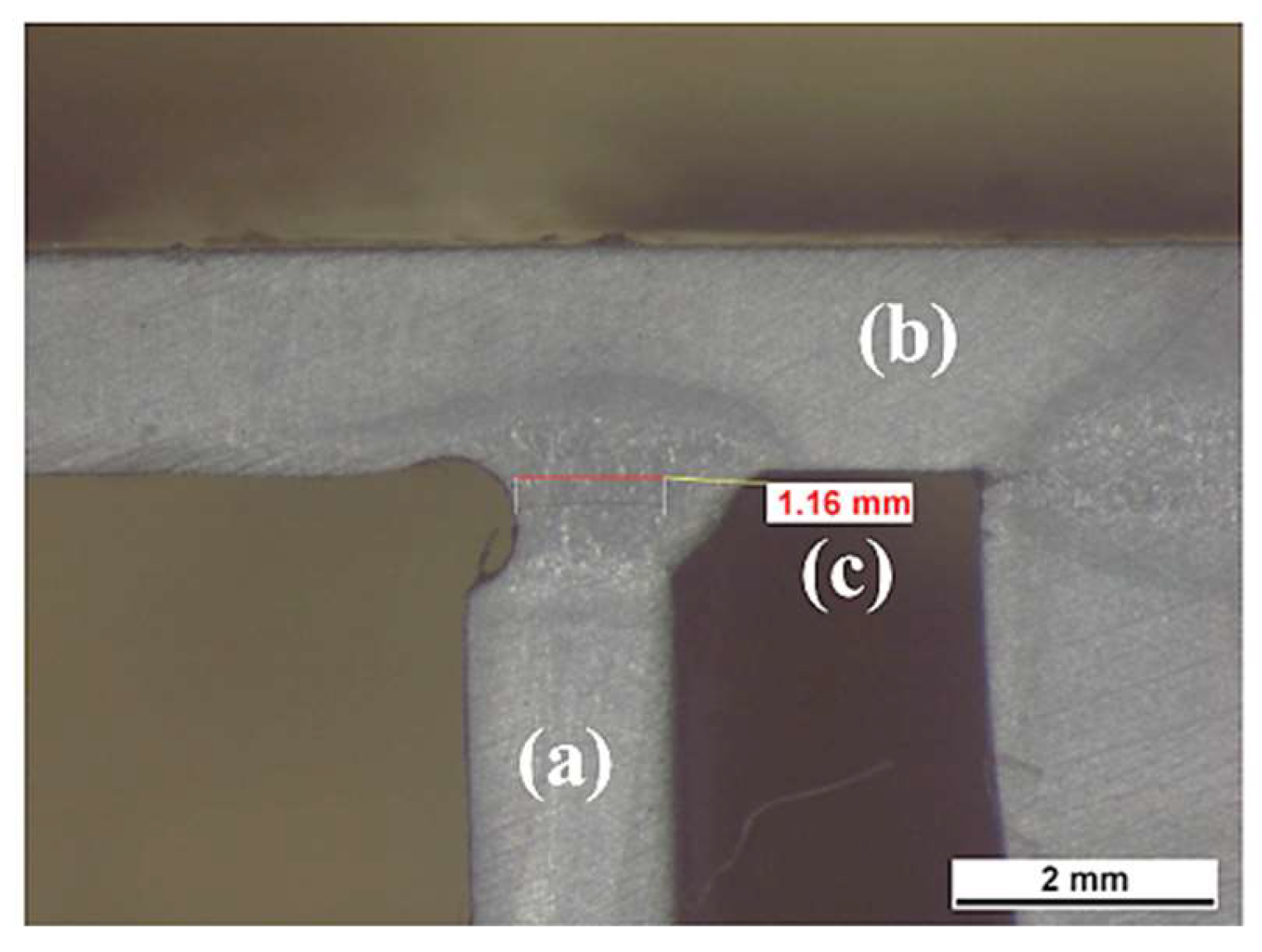
Figure 3.
PDCA framework application for the process improvement for the weld penetration depth (y).
Figure 3.
PDCA framework application for the process improvement for the weld penetration depth (y).
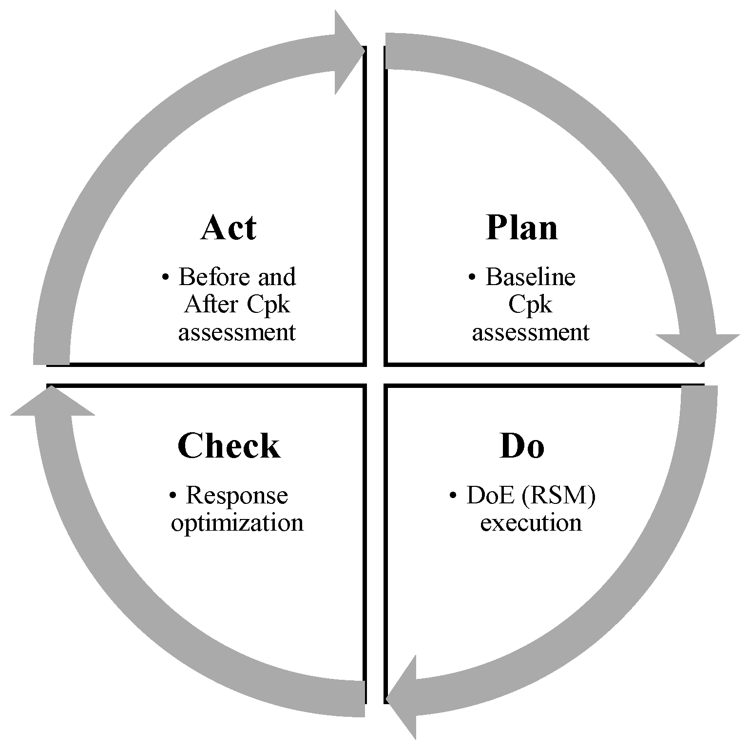
Figure 4.
Baseline process capability assessment for weld depth penetration (mm), where the penetration depth (y) specification is a minimum of 1.20 mm, the average depth is 1.246 mm with a standard deviation of 0.0306 mm, and Cpk = 0.50.
Figure 4.
Baseline process capability assessment for weld depth penetration (mm), where the penetration depth (y) specification is a minimum of 1.20 mm, the average depth is 1.246 mm with a standard deviation of 0.0306 mm, and Cpk = 0.50.
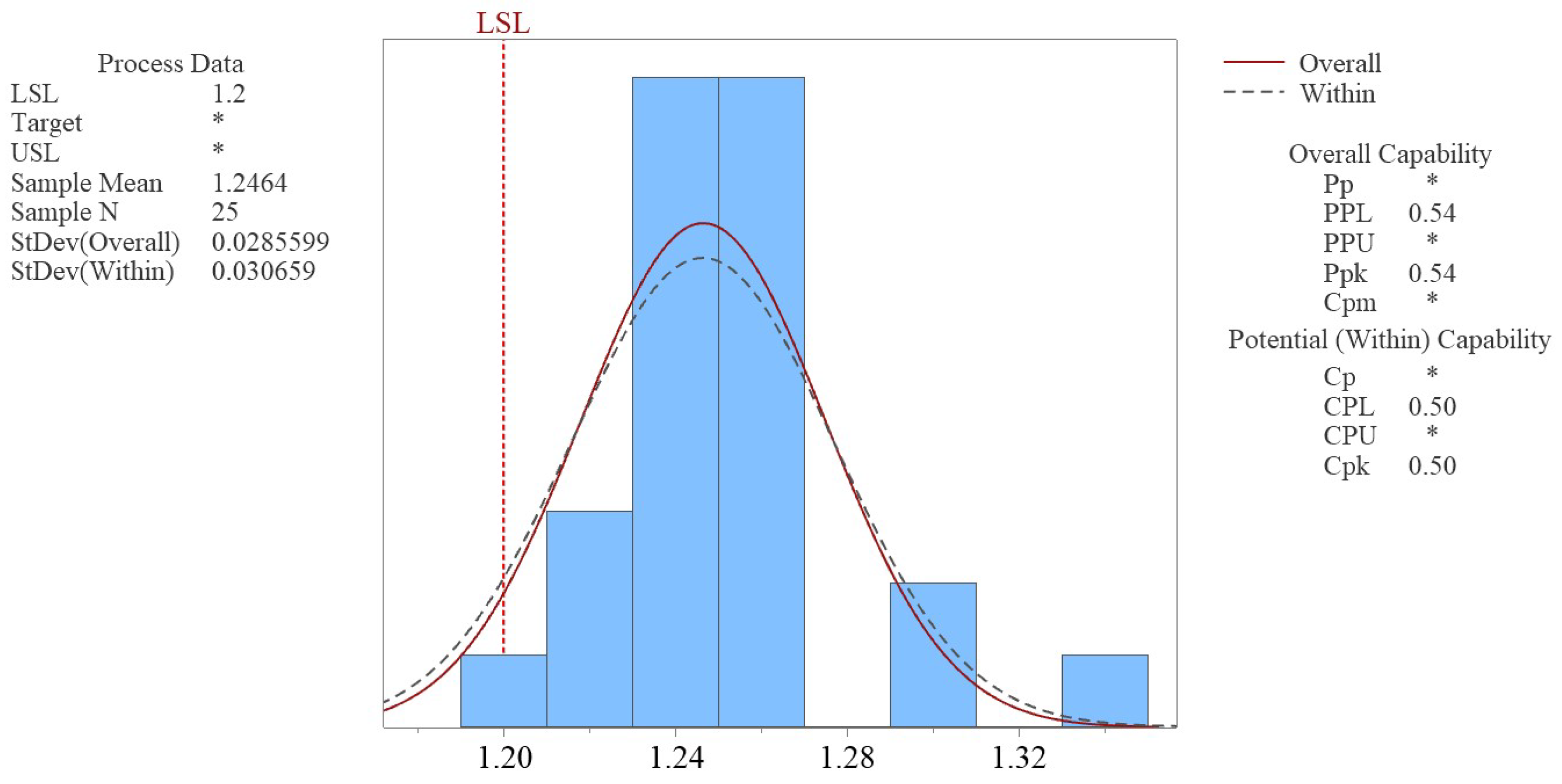
Figure 5.
Half-normal plot of standardized effects on weld penetration depth.

Figure 6.
Contour plots for weld penetration depth (y) in [mm], using Equation (2). a) B–A relationship when C = 0; b) C–A relationship when B = 0; c) C–B relationship when A = 0.
Figure 6.
Contour plots for weld penetration depth (y) in [mm], using Equation (2). a) B–A relationship when C = 0; b) C–A relationship when B = 0; c) C–B relationship when A = 0.
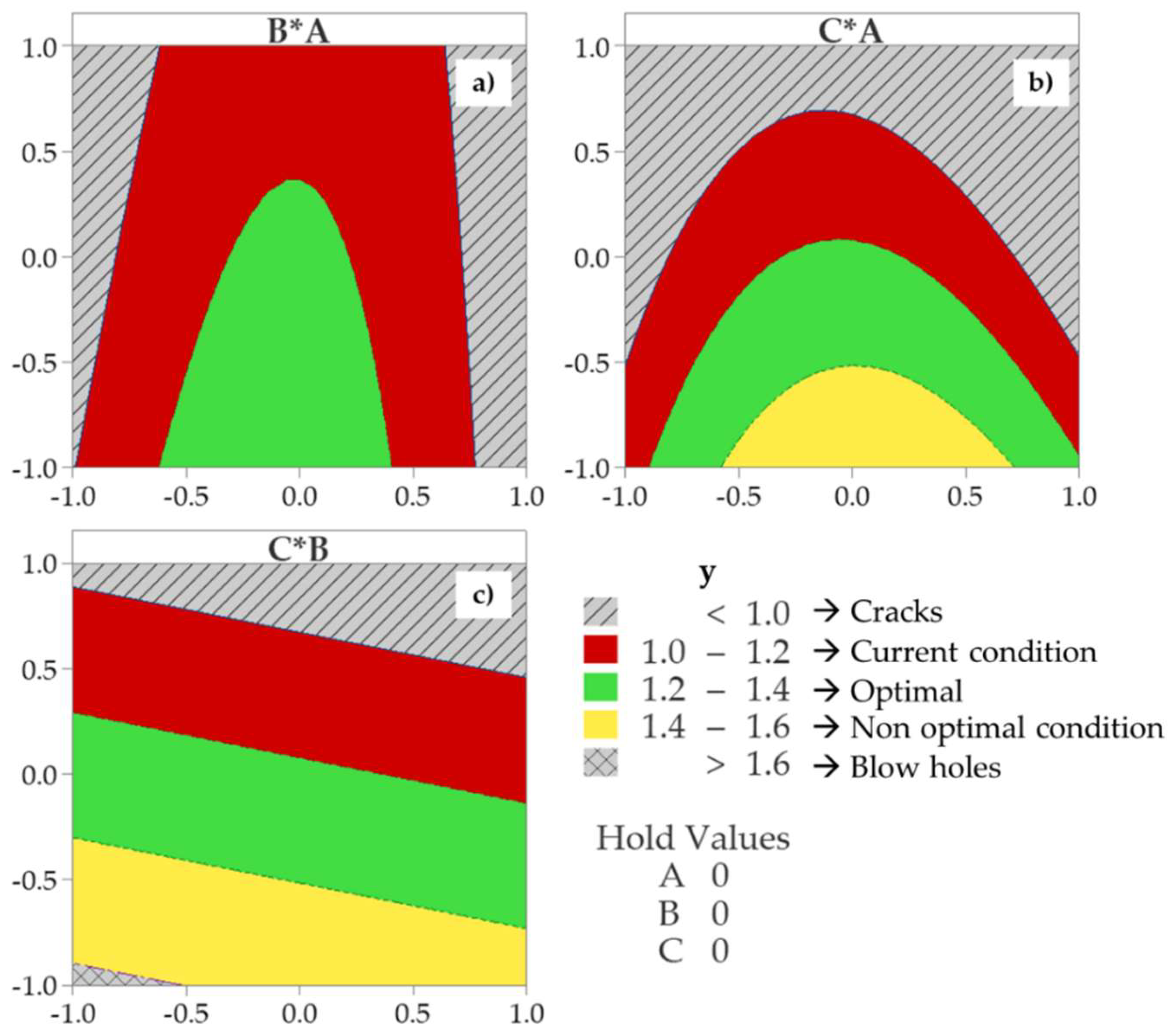
Figure 7.
Ground and polished macrograph of ZE 790 steel welded by LBW after proposed parameters, using RSM: (a) Side panel thickness, (b) upper rail thickness, and (c) weld depth penetration greater than minimum specification (1.2 mm).
Figure 7.
Ground and polished macrograph of ZE 790 steel welded by LBW after proposed parameters, using RSM: (a) Side panel thickness, (b) upper rail thickness, and (c) weld depth penetration greater than minimum specification (1.2 mm).
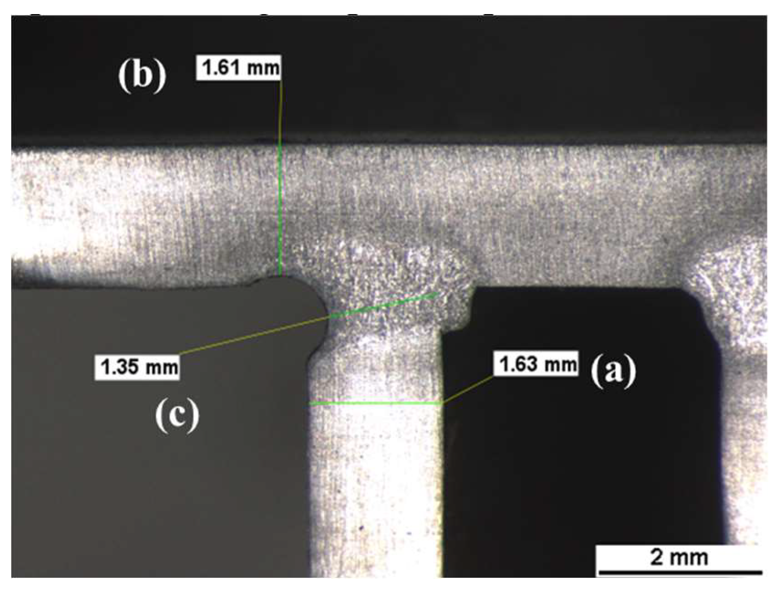
Figure 8.
Weld depth penetration (mm), process comparison before and after parameters adjustment; considering different batches of raw material and production shifts. *Minimum material thickness.
Figure 8.
Weld depth penetration (mm), process comparison before and after parameters adjustment; considering different batches of raw material and production shifts. *Minimum material thickness.

Table 1.
Comparison of proposed methods to control weld penetration using laser beam welding (LBW) machines.
Table 1.
Comparison of proposed methods to control weld penetration using laser beam welding (LBW) machines.
| Characteristics evaluated by authors | Madrid et al. [7] | Schmoeller et al. [9] | Dos-Santos-Paes et al. [27] | Pavlicek et al. [28] | Khorram et al. [29] | Yufeng et al. [30] | Krishna-Kumar et al. [31] | Khann et al. [32] | Our Proposed |
|---|---|---|---|---|---|---|---|---|---|
| Output variable(s): | |||||||||
| Weld penetration | ☒ | ☒ | ☒ | ☒ | ☒ | ☒ | ☒ | ☒ | ☒ |
| Input variable(s): | |||||||||
| Power | ☐ | ☒ | ☒ | ☒ | ☒ | ☒ | ☒ | ☒ | ☒ |
| Speed | ☒ | ☒ | ☒ | ☒ | ☒ | ☒ | ☒ | ☒ | ☒ |
| Focal position | ☒ | ☐ | ☐ | ☒ | ☒ | ☒ | ☒ | ☒ | ☒ |
| Joint thickness | ☒ | ☐ | ☐ | ☒ | ☒ | ☒ | ☒ | ☒ | ☒ |
| Proposed methodology for analysis: | |||||||||
| Empirical experimentation | ☐ | ☐ | ☒ | ☐ | ☐ | ☐ | ☐ | ☒ | ☐ |
| Analysis of one factor at a time | ☐ | ☐ | ☒ | ☐ | ☐ | ☐ | ☐ | ☐ | ☐ |
| Design of experiments | ☒ | ☐ | ☐ | ☐ | ☒ | ☒ | ☒ | ☒ | ☒ |
| Finite element analysis | ☐ | ☐ | ☐ | ☒ | ☐ | ☐ | ☐ | ☐ | ☐ |
| Artificial neural networks | ☐ | ☒ | ☐ | ☐ | ☐ | ☐ | ☐ | ☐ | ☒ |
| Solution model: | |||||||||
| Linear model | ☐ | ☒ | ☒ | ☐ | ☐ | ☒ | ☐ | ☒ | ☐ |
| Quadratic model | ☐ | ☐ | ☐ | ☒ | ☒ | ☐ | ☒ | ☐ | ☒ |
| Model with interactions | ☐ | ☐ | ☐ | ☐ | ☐ | ☐ | ☒ | ☒ | ☒ |
| Model validation | ☒ | ☒ | ☐ | ☒ | ☒ | ☐ | ☒ | ☒ | ☒ |
| Calculation of process capability | ☐ | ☐ | ☐ | ☐ | ☐ | ☐ | ☐ | ☐ | ☒ |
| Actual implementation: | |||||||||
| The improvement is implemented | ☐ | ☐ | ☐ | ☐ | ☐ | ☐ | ☐ | ☐ | ☒ |
Table 2.
Chemical composition of ZE 790 steel (wt. %).
| Material | C | Si | Mn | P | S | Cr | Mo | Ni | Cu | Al | V |
|---|---|---|---|---|---|---|---|---|---|---|---|
| ZE 790 | 0.060 | 0.030 | 0.540 | 0.007 | 0.000 | 0.070 | 0.020 | 0.050 | 0.140 | 0.037 | 0.008 |
Table 3.
Process parameters of the LBW machine for the DoE.
| Parameter 1 | Process Range |
|---|---|
| A – Welding speed (mm/s) | 22–30 |
| B – Laser power (W) | 2000–3000 |
| C – Focal position Z-axis (mm) | 223.80–224.50 |
1 Focal position (X-axis) = 115.00 mm; slope angle = −1.36°; beam angle = 8.48°.
Table 4.
Codification of input variables and experimental levels definition for the DoE.
| Code | Factor | -1 | 0 | +1 |
|---|---|---|---|---|
| A | Welding speed (mm/s) | 22 | 30 | 38 |
| B | Laser power (W) | 2,000 | 2,500 | 3,000 |
| C | Focal Position Z-axis (mm) | 223.80 | 224.15 | 224.50 |
Table 5.
Weld penetration depth (y) [mm] tally sheet from DoE.
| Treatment | A | B | C | Sample 1 | Sample 2 | Sample 3 |
|---|---|---|---|---|---|---|
| 1 | −1 | −1 | −1 | 1.25 | 1.26 | 1.25 |
| 2 | +1 | −1 | −1 | 1.08 | 1.29 | 1.18 |
| 3 | -1 | +1 | −1 | 1.08 | 0.95 | 0.91 |
| 4 | +1 | +1 | −1 | 1.30 | 1.24 | 1.25 |
| 5 | −1 | −1 | +1 | 0.64 | 0.69 | 0.85 |
| 6 | +1 | −1 | +1 | 0.58 | 0.44 | 0.37 |
| 7 | −1 | +1 | +1 | 0.42 | 0.55 | 0.60 |
| 8 | +1 | +1 | +1 | 0.22 | 0.44 | 0.18 |
| 9 | 0 | 0 | 0 | 1.24 | 1.23 | 1.21 |
Table 6.
ANOVA results.
| Source | DF | SS | MS | F-Value | P-Value |
|---|---|---|---|---|---|
| Model | 6 | 3.52272 | 0.58712 | 58.84 | 0.000 |
| Linear | 3 | 2.86523 | 0.95508 | 95.72 | 0.000 |
| A | 1 | 0.03227 | 0.03227 | 3.23 | 0.087 |
| B | 1 | 0.12615 | 0.12615 | 12.64 | 0.002 |
| C | 1 | 2.70682 | 2.70682 | 271.29 | 0.000 |
| Square | 1 | 0.41082 | 0.41082 | 41.17 | 0.000 |
| A*A | 1 | 0.41082 | 0.41082 | 41.17 | 0.000 |
| Two-way int. | 2 | 0.24667 | 0.12333 | 12.36 | 0.000 |
| A*B | 1 | 0.05227 | 0.05227 | 5.24 | 0.033 |
| A*C | 1 | 0.19440 | 0.19440 | 19.48 | 0.000 |
| Error | 20 | 0.19955 | 0.00998 | ||
| Lack of fit | 2 | 0.05568 | 0.02784 | 3.48 | 0.053 |
| Pure error | 18 | 0.14387 | 0.00799 | ||
| Total | 26 | 3.72227 |
Table 7.
Coefficients (coded) of the regression equation2.
| Term | Coef | SE Coef | T-Value | P-Value | VIF |
|---|---|---|---|---|---|
| Constant | 1.2267 | 0.0577 | 21.27 | 0.000 | |
| A | −0.0367 | 0.0204 | −1.80 | 0.087 | 1.00 |
| B | −0.0725 | 0.0204 | −3.56 | 0.002 | 1.00 |
| C | −0.3358 | 0.0204 | −16.47 | 0.000 | 1.00 |
| A*A | −0.3925 | 0.0612 | −6.42 | 0.000 | 1.00 |
| A*B | 0.0467 | 0.0204 | 2.29 | 0.033 | 1.00 |
| A*C | −0.0900 | 0.0204 | −4.41 | 0.000 | 1.00 |
2 R-sq = 0.94, Rs-q(adj) = 0.93, R-sq(pred) = 0.90.
Table 8.
Regulatory conditions for the operation of the welding process for y ≈ 1.35 mm3.
| Parameter | Coded | Non-Coded |
|---|---|---|
| A – Welding speed (mm/s) | 0 | 30 |
| B – Laser power (W) | 0 | 2500 |
| C – Focal position Z-axis (mm) | −0.3672 | 224.02 |
3 Optimal process parameters that ensure weld integrity without cracks or blow holes.
Table 9.
Process capability assessment for the specification of a minimum y of 1.20 mm.
| Process | N | Mean (mm) | StDev (mm) | Min (mm) | Max (mm) | Cpk | % Out of Spec | ppm |
|---|---|---|---|---|---|---|---|---|
| Before* | 25 | 1.2464 | 0.0307 | 1.1600 | 1.3100 | 0.50 | 6.51 | 65,086 |
| After * | 11 | 1.3536 | 0.0284 | 1.2700 | 1.4200 | 1.81 | 0.00 | 0 |
*Optimization.
Disclaimer/Publisher’s Note: The statements, opinions and data contained in all publications are solely those of the individual author(s) and contributor(s) and not of MDPI and/or the editor(s). MDPI and/or the editor(s) disclaim responsibility for any injury to people or property resulting from any ideas, methods, instructions or products referred to in the content. |
© 2024 by the authors. Licensee MDPI, Basel, Switzerland. This article is an open access article distributed under the terms and conditions of the Creative Commons Attribution (CC BY) license (http://creativecommons.org/licenses/by/4.0/).
Copyright: This open access article is published under a Creative Commons CC BY 4.0 license, which permit the free download, distribution, and reuse, provided that the author and preprint are cited in any reuse.


