
Submitted:
10 October 2024
Posted:
10 October 2024
You are already at the latest version
Abstract
Different researchers analyzed effective computational methods that maintain the precision of Allen-Chan (AC) equations and their constant security. This article presents a method known as reduced order model technique by utilizing kernel principle component analysis (KPCA), a nonlinear variation of traditional principal component analysis (PCA). KPCA is utilized on the data matrix created using discrete solution vectors of the AC equation. In order to achieve discrete solutions, small variations are applied for dividing up extraterrestrial elements, while Kahan’s method is used for temporal calculations. Handling the process of backmapping from small-scale space involves utilizing a non-iterative formula rooted in the concept of the multi-dimensional scaling (MDS) method. Using KPCA, we show that simplified sorting methods preserve dissipation of energy structure. The effectiveness of simplified solutions from linear PCA and KPCA, the retention of invariants, and computational speeds are shown through one-, two-, and three-dimensional AC equations.
Keywords:
Allen-Cahn equation
; kernel principle component analysis
; multi-dimensional scaling
; energy dissipation
MSC: 68T99; 65F55
1. Introduction
Differential equations, particularly partial differential equations (PDEs), are commonly used to mathematically represent most real-life problems in different scientific fields. Among them the Allen-Chan (AC) equation is a popular nonlinear PDE for modeling phase transition issues. The AC equation was firstly presented in [1] to simulate the movement of antiphase boundaries in crystalline solids. The AC equation is commonly applied to represent different natural phenomena and has become a fundamental equation for the diffuse interface method used to investigate phase transitions and interfacial dynamics in various fields such as materials science [2], image analysis [3], fluid dynamics [4] and mean curvature flow [5]. In materials science, it is used to simulate phase transformations in polymer, metal and ceramic materials [6]. AC equation is further used in multi-reconstruction [7] and predicting the evolution of microstructures in various materials and also in biophysics [8].
The AC equation define by
explains the movement of the anti-phase borders of a dual metal mixture at a set temperature. In equation (1), is used to denote the amount of one metal component in the alloy while the positive parameter represents the narrow inter-facial width that is smaller than the lab scale length. We examine the AC equation (1) on a domain , (), enforced with homogeneous Neumann or periodic boundary conditions, and with the double-well potential . The nonlinear functional in (1) is given as , and the free energy functional of the AC equation is defined by
In this form, the AC equation (1) is a dissipative gradient system
where represents the variational derivative of the free energy. In other words, the AC equation meets a non-linear stability condition, which means that the free energy functional decreases over time, i.e., for .
Dimensionality reduction for dynamical systems is a crucial process aimed at simplifying complex models while retaining the essential features of their behavior. In many real-world applications, such as fluid dynamics, climate modeling, and biological systems, the state space can be incredibly high-dimensional, making simulations computationally expensive and difficult to analyze. Intrusive and data-driven reduced order modeling (ROM) are two distinct approaches used for dimensionality reduction. Intrusive ROM relies on integrating reduced models directly into the numerical algorithms of the original system, often requiring detailed knowledge of the governing equations. In contrast, data-driven ROM leverages discrete data to construct models, utilizing techniques like machine learning and statistical analysis to capture system behavior without explicit knowledge of the underlying physics. Among them, principal component analysis (PCA) is a robust statistical method used for reducing dimensionality and visualizing data across fields like image processing, genetics, finance, and social sciences. It transforms original variables into principal components that maximize variance, aiming to create a lower-dimensional representation while retaining original variability [9,10]. PCA’s effectiveness diminishes when data distributions exhibit low variance, making it less suitable for linear subspace decomposition.
Recently, kernel principal component analysis (KPCA) has emerged as an advanced alternative, which is an extension of traditional PCA that enables the analysis of nonlinear relationships within high-dimensional data. By employing a kernel function, KPCA implicitly maps the original data into a higher-dimensional feature space where linear separability is often achieved, allowing for more effective dimensionality reduction and feature extraction. This method excels in capturing complex patterns that conventional PCA might overlook, making it particularly useful in fields such as exploratory data analysis, pattern recognition, face recognition, manifold learning across fields like computer vision, bio-informatics, broad learning systems, and signal processing [11,12,13,14,15,16,17,18]. However, KPCA faces challenges in interpreting results in the original input space and the computational cost associated with kernel evaluations, with multidimensional scaling (MDS) being a notable approach for this purpose [14,19,20]. MDS allows for the iterative computation of the pre-image by employing various distance metrics between the data vectors. Despite these challenges, KPCA remains a powerful tool for exploratory data analysis and is widely utilized in applications
This paper explores the application of KPCA to data that derived from discrete solution vectors of the AC equation, a novel approach in ROM that preserves solution accuracy and conservation of energy dissipation property of the AC equation. In the literature, there are rare papers dealing with the ROM for AC equation. An energy stable ROM using finite differences and convex splitting, is derived for AC equation in [21], and a non-linear POD/Galerkin ROM is applied in [22]. In [23], the authors derive an energy stable ROM for AC equation using discontinuous Galerkin and average vector field methods, utilizing proper orthogonal decomposition-greedy adaptive sampling and discrete empirical interpolation method.
In the sequel, the paper outlines the AC equation’s mathematical formulation with space/time discretization in Section 2, details the KPCA process in Section 3, showcases results related to reduced solution accuracy and computational efficiency for the one-, two- and three-dimensional AC equations in Section 4, and concluding with key findings.
2. Discrete Data from AC Equation
Here, we present the spatio-temporal (full) discrete representation of the AC equation based on its free energy (2), where the solution vectors are utilized to construct the data set for further analysis.
The AC equation is first discretized in space. With this goal in mind, we employ finite difference discretization to the second order differentiation (Laplace) operator in AC equation utilizing a tensor framework. Let the matrix denotes the discrete Laplace operator, where the number m stands for the total degrees of freedom on the d-dimensional spatial mesh (. Let also the matrix stands, under periodic boundary conditions, for the matrix corresponding to the discretization of the Laplace operator by finite differences on a one-dimensional spatial interval consisting of grid points with the mesh size , given by
Firstly, consider a one-dimensional domain that partitioned into uniform subintervals with the mesh size . On this grid, simply, we have that and . On a two-dimensional rectangular domain that partitioned into and uniform subintervals with the mesh sizes and in either and coordinates, respectively, we can take the matrix A of discrete Laplace operator as
On a three-dimensional cuboid , on the other hand, let the domain is partitioned into , and uniform subintervals with the mesh sizes , and in either , and coordinates, respectively. Then, the matrix A of discrete Laplace operator is of the form
In the above setting, ⊗ denotes the Kronecker product and is the identity matrix of size , . We note that the matrix , and hence the matrix A, can be easily formed under homogeneous Neumann boundary condition; all we need is setting the most upper-right and the most bottom-left corner entries of the matrix to zero, and take .
After, we establish time-varying semi-discrete solution vector as
with representing the approximate solution at time t and i-th grid node of the partitioned mesh of the domain , in an appropriate order. After spatial discretization, we obtained the m-dimensional semi-discrete (dynamical) system
where is the ordinary differentiation with respect to time variable t, and the m-dimensional vector is such that , .
The full discrete system for the AC equation is derived by applying a temporal integration technique to the semi-discrete system (3). Since the effective non-intrusive dimension reduction methods rely on an accurate and reliable data, and the data set used in this paper is composed of the discrete solution vectors of the full discrete system of the AC equation, it is crucial to use a temporal integration that is both accurate and preserves the energy dissipation property of the AC equation. An energy-stable scheme is a numerical method that maintains the energy dissipation/conservation of a gradient/Hamiltonian flow at the discrete level. Extensive literature exists on gradient stable schemes for the AC equation. In this instance, we utilize Kahan’s method [24], which is an advanced numerical method designed to enhance the accuracy of time integration for dynamic systems. Kahan time integrator achieves higher precision compared to traditional integration methods, such as the standard Runge-Kutta or Euler methods. It is a second order, time-reversal, and linearly implicit technique for ODEs [24].
For the full discrete system, we partition the time interval into equal parts with time step-size to create discrete time points , . The solution vector at time is denoted by . Then, the application of Kahan’s method leads to the full discrete problem: given by the initial condition, compute from the linear system
where is the right-hand side vector of the dynamical system (3), and is its diagonal Jacobian matrix. Under the given discretization, the discrete form of the energy reads as
where the matrix mimics the first order forward finite difference differentiation.
3. Reduced Order Model
In this part, we will cover the linear/nonlinear ROM formulation of the AC equation. First, we briefly outline the conventional PCA method, followed by an explanation of KPCA, the nonlinear counterpart of the PCA. The process involves two steps: starting with vectors from the column space of a data matrix, known as the input space, moving to the reduced space via projection, and then mapping back from the reduced space to the input space to get the reduced approximation. Because the ROM approach we are examining relies on a given data, we will focus in the following sections on the data matrix
where the column vectors represent the solution vectors of the AC equation derived from the full discrete system (4). We make a point to simplify notation by beginning the initial superscript of the snapshot vectors in equation (6) at 1 instead of 0. This means that the column vector in equation (6) corresponds to the solution vector , , of the AC equation derived from the system (4).
3.1. Linear Dimension Reduction (PCA)
In the case of a data matrix (6) containing the solution vectors for AC equation, PCA aims to find a linear model of a reduced dimension , which can accurately represent the variance in the vectors . We assume that the matrix U has zero column sum, otherwise, we can achieve this by subtracting the average column value from each column. The covariance matrix C of the matrix U is defined by
whose diagonalization is given by
where the column vectors of the orthogonal matrix represent the eigenvectors related to the (sorted) eigenvalues lined up on the diagonal entries of diagonal matrix . Next, the eigenvectors of the covariance matrix C with the k largest eigenvalues are considered as the basis of the k-dimensional linear subspace in a straightforward manner [17]. Ultimately, any random vector in the input space can be roughly expressed by the pre-image as a linear combination of the eigenvectors
with the matrix being composed of the initial k columns of the orthogonal matrix P. The reel coefficients represent the components of the projection vector , obtained by projecting onto the smaller linear subspace. The dimensional vector lies in the reduced space, which is the projection of the m-dimensional vector from the input space [25].
3.2. Nonlinear Dimension Reduction (KPCA)
PCA is restricted to reducing dimensionality in a linear manner. However, standard PCA may be inefficient when confronted with data featuring intricate structures that cannot be accurately represented within a linear subspace. Yet, KPCA provides a resolution by allowing us to expand the linear PCA for nonlinear dimensionality reduction [12,14,16].
By utilizing KPCA, one maps the vectors from the m-dimensional input space to a larger dimensional (potentially infinite-dimensional) space known as the feature space, through a nonlinear map . Then, the traditional PCA is subsequently implemented on the vectors within this feature space. In order to achieve this, we label as the converted data matrix created as
where the columns consist of the converted vectors corresponding to the input space vectors . In most cases, the matrix , associated with the arbitrary map , does not necessarily possess zero column sum for PCA. Subtracting the mean from each column results in a data matrix
with zero column sum, where the columns are , and H is the centering matrix defined by
where is the n-dimensional identity matrix and is the vector of ones. Next, we apply the standard PCA steps described earlier, to the data matrix which has columns that represent the feature space. This involves identifying the eigenvectors of the covariance matrix
Currently, the KPCA has two significant disadvantages. In the first place, the size M could be so large that it becomes nearly impossible to calculate the eigenvectors of the M-dimensional covariance matrix . Second, the random nonlinear function is often inaccessible. To tackle these problems, a kernel trick is utilized [16,17]. To comprehend this technique, let’s examine the eigenvalue problem
where represent the eigenpair of the covariance matrix . It is important to understand that, by definition, the eigenvectors cover the feature space, which is equivalent to the column space of the altered data matrix . Consequently, there are real coefficients for each eigenvector that satisfy the linear combination
By replacing the connection (11) and the identity (9) into the equation (10), we get that
All eigenvectors are within the range of the altered vectors , so for , we can examine the equivalent equations by projecting onto the vectors , resulting in
At this stage, a kernel function is defined so that
with the goal of depicting the Euclidean inner products of non-centered transformed vectors in the feature space using input space vectors. Different types of kernel functions are utilized in various studies, including linear, polynomial, and Gaussian kernels [16,25]. Here, we employ the Gaussian kernel defined for any vector by
where represents the Euclidean norm and being a parameter.
In addition, to depict the Euclidean inner products of transformed vectors that are centered in the feature space, we utilize the framework [14]
where the kernel matrix , and the vector are defined as
We note that it is not necessary to compute all the vectors , as they are simply the ith columns of the symmetric kernel matrix K. The use of the kernel function results in an equivalent equation to (12) being
The equation (13) can be represented in matrix-vector form as
for the coefficient vector , where and H is the centering matrix given in (8). Ultimately, for any vector in the input space, its transformed vector in the feature space is found. The projection vector represents the projection of onto the reduced k-dimensional space () spanned by the eigenvectors associated with the largest k eigenvalues . After calculating the coefficients from the eigenvalue problem (14) and utilizing the identity (11) of the eigenvectors , the projection vectors’ entries can be determined using the kernel function as the following
Reconstructing the original image of any random vector in the input space can be achieved by approximating its pre-image using standard PCA as shown in equation (7). Nonetheless, KPCA does not follow this pattern. Denote as the projection of onto the reduced space spanned by the eigenvectors , namely
Next, we can find an estimated pre-image such that the vector after transformation is the vector closest to the projected vector . This involves determining the minimum of the objective functional using a least-squares approach. By imposing , we obtain the following equation to be solved
where we set
The implicit equation (15) can be solved by fixed-point iteration or other Newton type nonlinear iterative solvers. But, the nonlinear iteration technique is unstable and depends highly on the initial estimation [14,25]. In the KPCA method presented in this study, the pre-image is calculated using a non-iterative approach [14], which relies on the correlation between the distance of vectors in the input space and the distance of the vectors in the transformed space, employing the Gaussian kernel function as a distance metric function . By utilizing MDS concept [14,19], we can roughly discover a pre-image where the differences in distances between and each input vector and between projected vector and each transformed feature vector remain constant, see Figure 1. To achieve this goal, let
represent the distance metrics between input space vectors and their transformed feature space vectors. After manipulating the Gaussian kernel function as , we can establish a relation between input space distance and feature space distance, and also its inverse map, as [14]
In addition, it can be demonstrated using the kernel matrix that the distance in feature space between the projected vector and a transformed vector is
for the matrix
Ultimately, by taking and utilizing the metric relation (16) within equation (15), we can derive the non-iterative solution formula [14]
where the distance in the formula is determined through relation (17). Furthermore, the k vectors mentioned in (18) are chosen from the n input space vectors that are closest to the given vector [14,25].
4. Numerical Results
In this section, we investigate how well the KPCA nonlinear dimensionality reduction method performs on one-, two- and three-dimensional AC equations. In either example, we construct the data matrix U whose columns are formed by the discrete solution vectors of the given AC equation, obtained by the full discrete system discussed in Section 2. In order to measure the accuracy of a reduced approximation to a fixed full solution , we use the relative absolute error defined by
4.1. One-Dimensional Problem
The AC equation (1) will be numerically modeled over the one-dimensional domain with periodic boundary conditions, and with the target time . The inter-facial width is set as , and the initial phase is
Data matrix U is created using discrete solutions at each time taken from the instant information of the system with space-time discretization, with the mesh sizes and [6]. The discretized data matrix for space and time coordinates is written as .
Figure 2 displays the plots of the precise solutions at , and also the solution trajectory for the time span . The AC equation with the potential function has one stable () and two unstable () equilibrium points. This phenomenon, known as phase separation, involves solutions transitioning between the equilibrium points. The boundaries separating the two unstable equilibrium zones shift across areas over extended periods, known as meta-stability. Figure 2, left, shows this state of meta-stability.
Table 1 compares PCA and KPCA methods in terms of accuracy and computational efficiency. For this comparison, the input space solution vector corresponding to the solution at time is used. Results are presented for reduced dimensions . The relative absolute errors between the full solution and the reduced approximate solution are shown when PCA and KPCA are used. When using the same number of reduced bases, more accurate results are obtained with KPCA.
On the other hand, in terms of computational efficiency, Table 2 shows the solution times required by the KPCA method using the formula (15), which is solved by fixed point iteration, and the method using the algebraic equation (18). The first two columns show the errors between the full and reduced solutions obtained with both formulae, while the last two columns show the processing time required to generate the preliminary images. It can be seen that the errors obtained with the solutions of the non-linear equation solved with iteration (2-3 iterations) with the formula (15) and without iteration with the formula (18) are almost the same, which shows that the solutions obtained without iteration are acceptable in terms of precision. It can be seen in the last two columns that the solution time required by the KPCA method without iteration is much less than the solution time required with iteration, i.e., the KPCA method is quite fast.
Figure 3 shows the reduced solutions together with the full solutions at times and . For the reduced dimension , it can be seen that the exact and reduced solutions coincide at both times. The full and reduced solution profiles are given in Figure 4. From the figures, it is observed that the full and reduced solutions coincide, and hence show the same phase transition behavior.
The energy graphs obtained with full solutions and preliminary images are given in Figure 5. It can be seen that the same energy reduction behavior is observed in both graphs.
4.2. Two-Dimensional Problem
The AC equation (1) will be numerically modeled over the two-dimensional domain with periodic boundary conditions, and with the target time . The inter-facial width is set as , and the initial condition is
Data matrix U is created using discrete solutions with the mesh sizes and [6]. The discretized data matrix for this setting is formed as .
Table 3 compares the PCA and KPCA methods in terms of accuracy and computational efficiency. For this comparison, the solution vector input space corresponding to the solution at time is used. Results are presented for reduced dimensions . The relative absolute errors between the exact solution and the reduced approximate solution are shown when PCA and KPCA are used. When using the same number of bases, more accurate results are obtained with KPCA.
In terms of computational efficiency, Table 4 shows the solution times required by the KPCA method using the formula (15) solved by fixed point iteration and the method using the algebraic equation (18). The first two columns show the errors between the full and reduced solutions obtained with both formulas, while the last two columns show the processing time required to generate the preliminary images. It can be seen that the errors obtained with the solutions of the non-linear equation solved with iteration (3 iterations) and without iteration are almost the same, which shows that the solutions obtained without iteration are acceptable in terms of precision. It can be seen in the last two columns that the solution time required by the KPCA method without iteration is considerably less than the solution time required with iteration.
Figure 6 shows the initial profile and profiles of the reduced solution together with the full solution at the final time . For the reduced dimension , the full and reduced solutions are similar. This means that the reduced solutions have the same behavior as the full one.
On the other hand, the energy plots obtained with full solutions and preliminary images are given in Figure 7. Here, it is clearly seen that the same energy reduction behavior occurs in both plots, similar to the one-dimensional AC equation.
4.3. Three-Dimensional Problem
In this last example, the scaled AC equation [6,26,27]
will be numerically modeled over the three-dimensional domain with homogenous Neumann boundary conditions, and with the target time . The inter-facial width is set as , and the initial condition is
Here, the given parameter represents the initial radius of the spherical zero isosurface, and at time t, the exact radius R of the sphere follows from the formula [26]. This indicates a decrease in the radius of the spherical zero isosurface over time. In the numerical simulation, we take the initial radius as .
For the discrete solution matrix U, we apply the mesh sizes and , i.e., the discretized data matrix is . Table 5 compares the PCA and KPCA methods in terms of accuracy and computational efficiency. For this comparison, the solution vector input space corresponding to the solution at time is used. Results are presented for reduced dimensions . The relative absolute errors between the full solution and the reduced approximate solution are shown when PCA and KPCA are used. When using the same number of bases, more accurate results are obtained with KPCA.
In terms of computational efficiency, Table 6 shows the solution times required by the KPCA method with and without iteration. It can be seen that the errors obtained with the solutions of the non-linear equation solved with iteration (2 iterations) and without iteration are almost the same, similar to the one- and two-dimensional cases, and that the KPCA method without iteration is fastest.
In Figure 8, left, the energy plots obtained with full and reduced solutions are given. Again, it is clearly seen that the same energy reduction behavior occurs by both full and reduced solutions. Figure 9 shows the profiles of the zero isosurface by full and reduced solutions at times . For the reduced dimension , the full and reduced profiles are highly similar, the radius of the spherical zero isosurface decrease as the time progresses. The decrease of the exact and numerical radii is also demonstrated in Figure 8, right.
5. Discussion
In this article, we suggest a nonlinear dimensionality reduction method that upholds precision and conserves the energy decay property of the one-, two-, and three-dimensional AC equations. The method for reducing dimensionality is non-intrusive and relies on the KPCA. The KPCA utilizes the MDS method and considers the input space and feature space distance metrics to develop a non-iterative algorithm for reconstructing pre-images. The numerical test examples show the accuracy of solutions and the preservation of energy dissipation structure. A comparison is made with traditional PCA and KPCA, as well as an iterative scheme with a non-iterative one. In our future research, we aim to explore various types of kernel functions that may offer more effective performance compared to the Gaussian kernel.
Author Contributions
Conceptualization, Y.Ç. and M.U.; methodology, Y.Ç. and M.U.; software, M.U.; validation, Y.Ç. and M.U.; formal analysis, Y.Ç. and M.U.; investigation, Y.Ç. and M.U.; resources, Y.Ç. and M.U.; data curation, M.U.; writing—original draft preparation, Y.Ç.; writing—review and editing, M.U.; visualization, Y.Ç. and M.U.; supervision, M.U.; project administration, Y.Ç. and M.U.; funding acquisition, Y.Ç. All authors have read and agreed to the published version of the manuscript.
Funding
This research received no external funding.
Data Availability Statement
Data sharing is not applicable.
Conflicts of Interest
The authors declare no conflicts of interest.
References
- Allen, S.M.; Cahn, J.W. A microscopic theory for antiphase boundary motion and its application to antiphase domain coarsening. Acta Metall 1979, 27, 1085–1095. [Google Scholar] [CrossRef]
- Chen, L.Q. Phase-field models for microstructure evolution. Annual Review of Materials Research 2002, 32, 113–140. [Google Scholar] [CrossRef]
- Benes̆, M.; Chalupecký, V.; Mikula, K. Geometrical image segmentation by the Allen-Cahn equation. Applied Numerical Mathematics 2004, 51, 187–205. [Google Scholar] [CrossRef]
- Yang, X.; Feng, J.J.; Liu, C.; Shen, J. Numerical simulations of jet pinching-off and drop formation using an energetic variational phase-field method. Journal of Computational Physics 2006, 218, 417–428. [Google Scholar] [CrossRef]
- Feng, X.; Prohl, A. Numerical analysis of the Allen-Cahn equation and approximation for mean curvature flows. Numerische Mathematik 2003, 94, 33–65. [Google Scholar] [CrossRef]
- Uzunca, M.; Karasözen, B. Linearly implicit methods for Allen-Cahn equation. Applied Mathematics and Computation 2023, 450. [Google Scholar] [CrossRef]
- Wang, J.; Shi, Z. Multi-Reconstruction from Points Cloud by Using a Modified Vector-Valued Allen–Cahn Equation. Mathematics 2021, 9, 1326. [Google Scholar] [CrossRef]
- Haq, M.U.; Haq, S.; Ali, I.; Ebadi, M.J. Approximate Solution of PHI-Four and Allen–Cahn Equations Using Non-Polynomial Spline Technique. Mathematics 2024, 12, 798. [Google Scholar] [CrossRef]
- Jackson, B.B.; Bund, B. Multivariate Data Analysis: An Introduction; From ThriftBooks-Atlanta (AUSTELL, GA, U.S.A., Richard D. Irwin, 1983.
- Johnson, R.; Wichern, D. Applied multivariate statistical analysis; New Jersey: Prentice-Hall, Michael Bell, 2007. [Google Scholar]
- Hached, M.; Jbilou, K.; Koukouvinos, C.; Mitrouli, M. A Multidimensional Principal Component Analysis via the C-Product Golub–Kahan–SVD for Classification and Face Recognition. Mathematics 2021, 9, 1249. [Google Scholar] [CrossRef]
- González, A.G.; Huerta, A.; Zlotnik, S.; Díez, P. A kernel Principal Component Analysis (kPCA) digest with a new backward mapping (pre-image reconstruction) strategy. Universitat Politecnica de Catalunya - Barcelona. [CrossRef]
- Mika, S.; Schölkopf, B.; Smola, A.; Müller, K.R.; Scholz, M.; Rätsch, G. Kernel PCA and De-Noising in Feature Spaces. Advances in Neural Information Processing Systems; Kearns, M.; Solla, S.; Cohn, D., Eds. MIT Press, 1998, Vol. 11.
- Rathi, Y.; Dambreville, S.; Tannenbaum, A. Statistical Shape Analysis using Kernel PCA. School of Electrical and Computer Engineering Georgia Institute of Technology 2006, 6064, 1–8. [Google Scholar] [CrossRef]
- Schölkopf, B.; Smola, A. Learning with kernels: support vector machines, regularization, optimization, and beyond; Adaptive computation and machine learning, MIT Press: Cambridge, Mass, 2002. [Google Scholar]
- Schölkopf, B.; Smola, A.; Müller, K.R. Nonlinear Component Analysis as a Kernel Eigenvalue Problem. Neural Computation 1998, 10, 1299–1319. [Google Scholar] [CrossRef]
- Wang, Q. Kernel Principal Component Analysis and its Applications in Face Recognition and Active Shape Models. Computer Vision and Pattern Recognition 2012, pp. 1–8. [CrossRef]
- Zhang, Q.; Ying, Z.; Zhou, J.; Sun, J.; Zhang, B. Broad Learning Model with a Dual Feature Extraction Strategy for Classification. Mathematics 2023, 11, 4087. [Google Scholar] [CrossRef]
- Cox, T.F.; Cox, M.A.A. Multidimensional Scaling; Monographs on Statistics and Applied Probability, Chapman & Hall: London, U.K., 2001. [Google Scholar]
- Williams, C.K.I. On a connection between kernel PCA and metric multidimensional scaling. Advances in Neural Information Processing Systems 13; Leen, T., Dietterich, T., Tresp, V., Eds.; MIT Press: Cambridge, MA, 2001. [Google Scholar]
- Song, H.; Jiang, L.; Li, Q. A reduced order method for Allen–Cahn equations. Journal of Computational and Applied Mathematics 2016, 292, 213–229. [Google Scholar] [CrossRef]
- Kalashnikova, I.; Barone, M.F. Efficient non-linear proper orthogonal decomposition/Galerkin reduced order models with stable penalty enforcement of boundary conditions. International Journal for Numerical Methods in Engineering 2012, 90, 1337–1362. [Google Scholar] [CrossRef]
- Uzunca, M.; Karasözen, B. Energy Stable Model Order Reduction for the Allen–Cahn Equation. In Model Reduction of Parametrized Systems; Benner, P., Ohlberger, M., Patera, A., Rozza, G., Urban, K., Eds.; Springer International Publishing: Cham, 2017; pp. 403–419. [Google Scholar] [CrossRef]
- Kahan, W.; Li, R.C. Unconventional Schemes for a Class of Ordinary Differential Equations. Journal of Computational Physics 1997, pp. 316–331. [CrossRef]
- Çakır, Y.; Uzunca, M. Nonlinear Reduced Order Modelling for Korteweg-de Vries Equation. International Journal of Informatics and Applied Mathematics 2024, 7, 57–72. [Google Scholar] [CrossRef]
- Li, Y.; Lee, H.G.; Jeong, D.; Kim, J. An unconditionally stable hybrid numerical method for solving the Allen-Cahn equation. Computers and Mathematics with Applications 2010, 60, 1591–1606. [Google Scholar] [CrossRef]
- Karasözen, B.; Uzunca, M.; Sariaydin-Filibelioğlu, A.; Yücel, H. Energy Stable Discontinuous Galerkin Finite Element Method for the Allen-Cahn Equation. International Journal of Computational Methods 2018, 15, 1850013 (26 pages). [Google Scholar] [CrossRef]
Figure 1.
Reconstruction with KPCA.
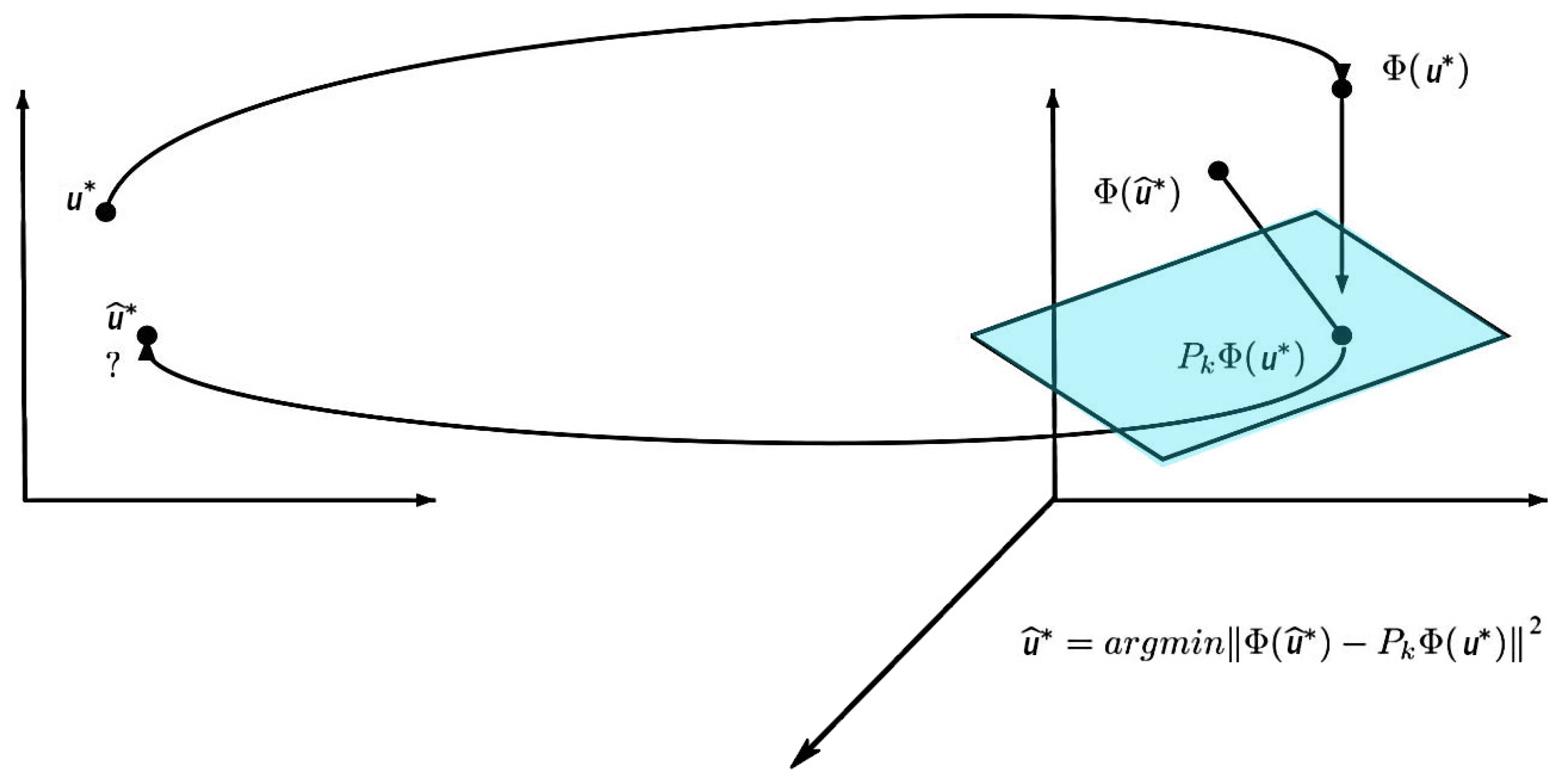
Figure 2.
1D AC: Phase trajectory (left) and phase plots (right) at times .
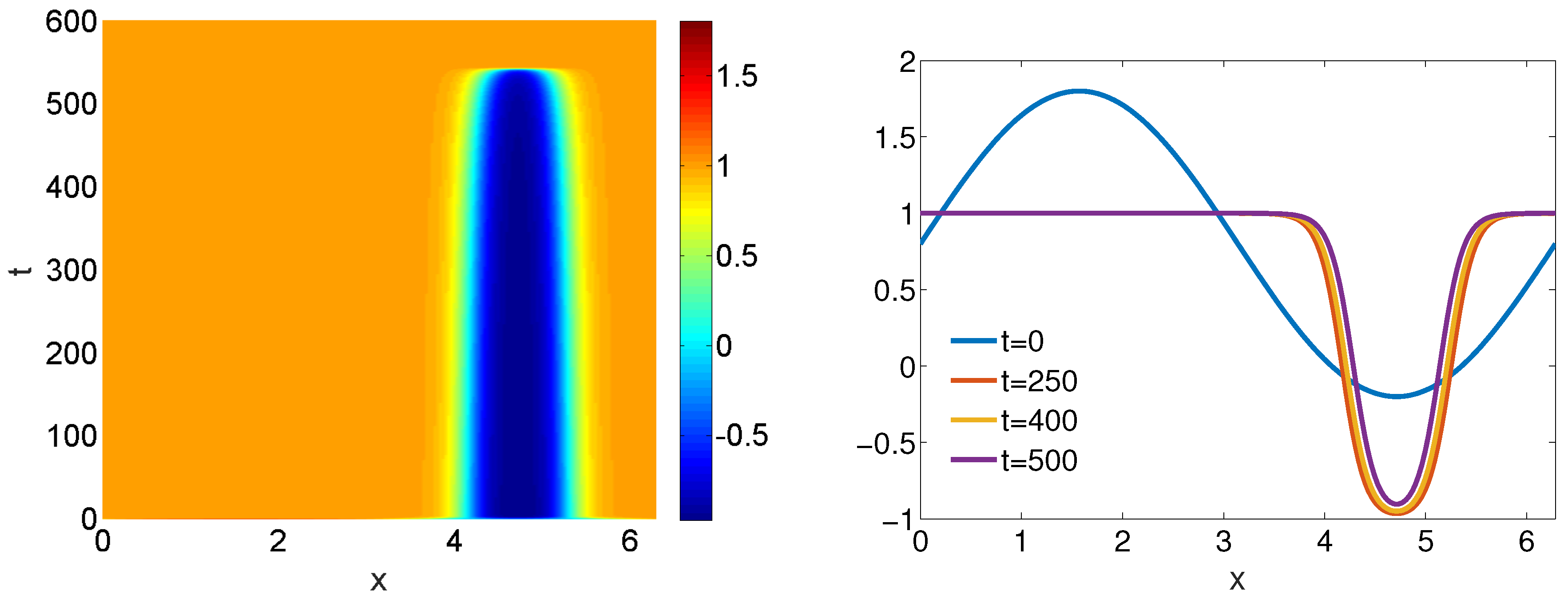
Figure 3.
1D AC: Full/reduced order solutions profiles at for .
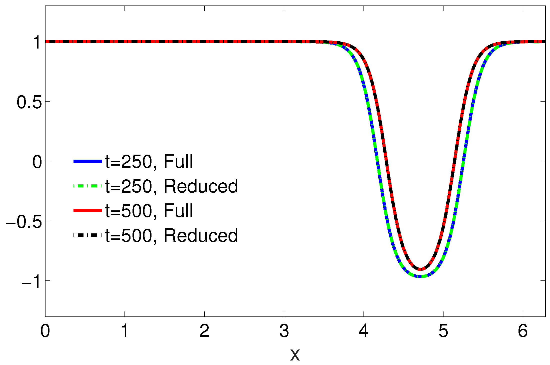
Figure 4.
1D AC: Full/reduced phase trajectories for .

Figure 5.
1D AC: Energy plots by full/reduced order solutions for .
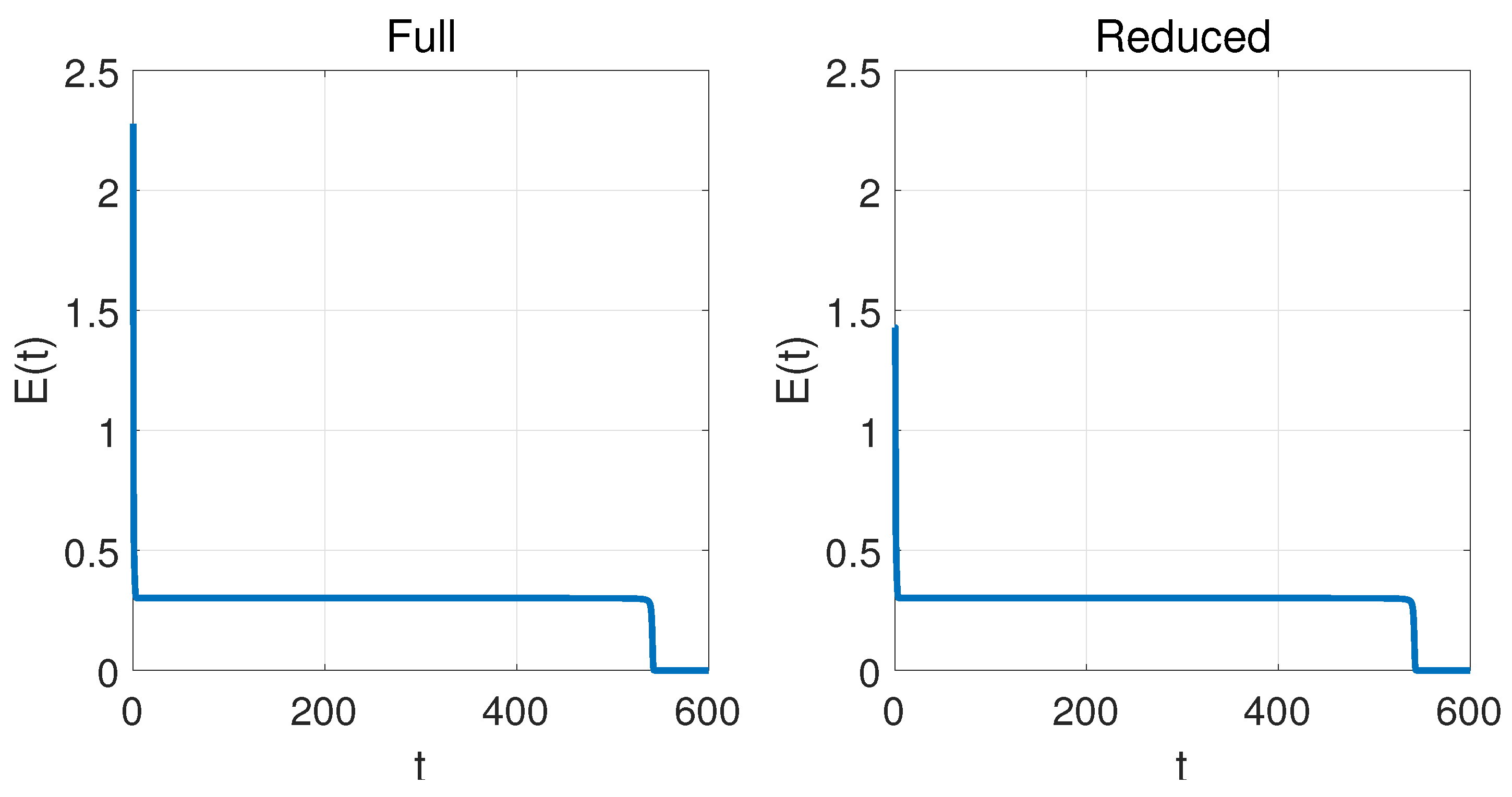
Figure 6.
2D AC: Full/reduced solution profiles for .
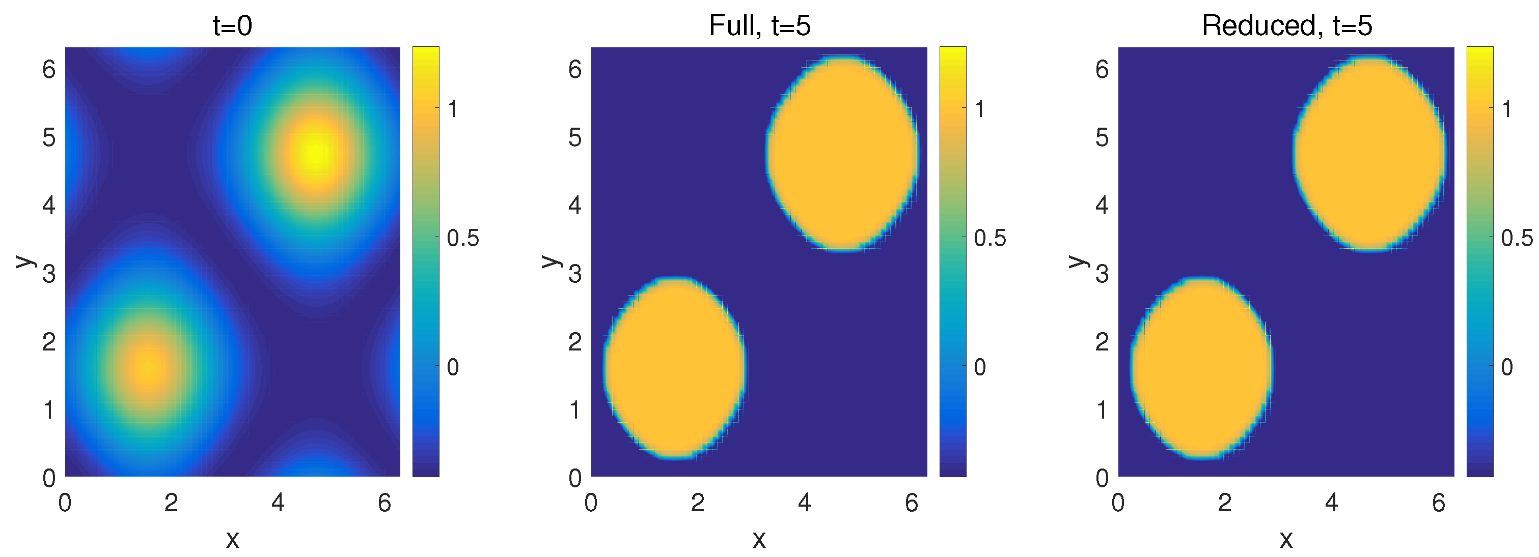
Figure 7.
2D AC: Energy plots by full/reduced order solutions for .
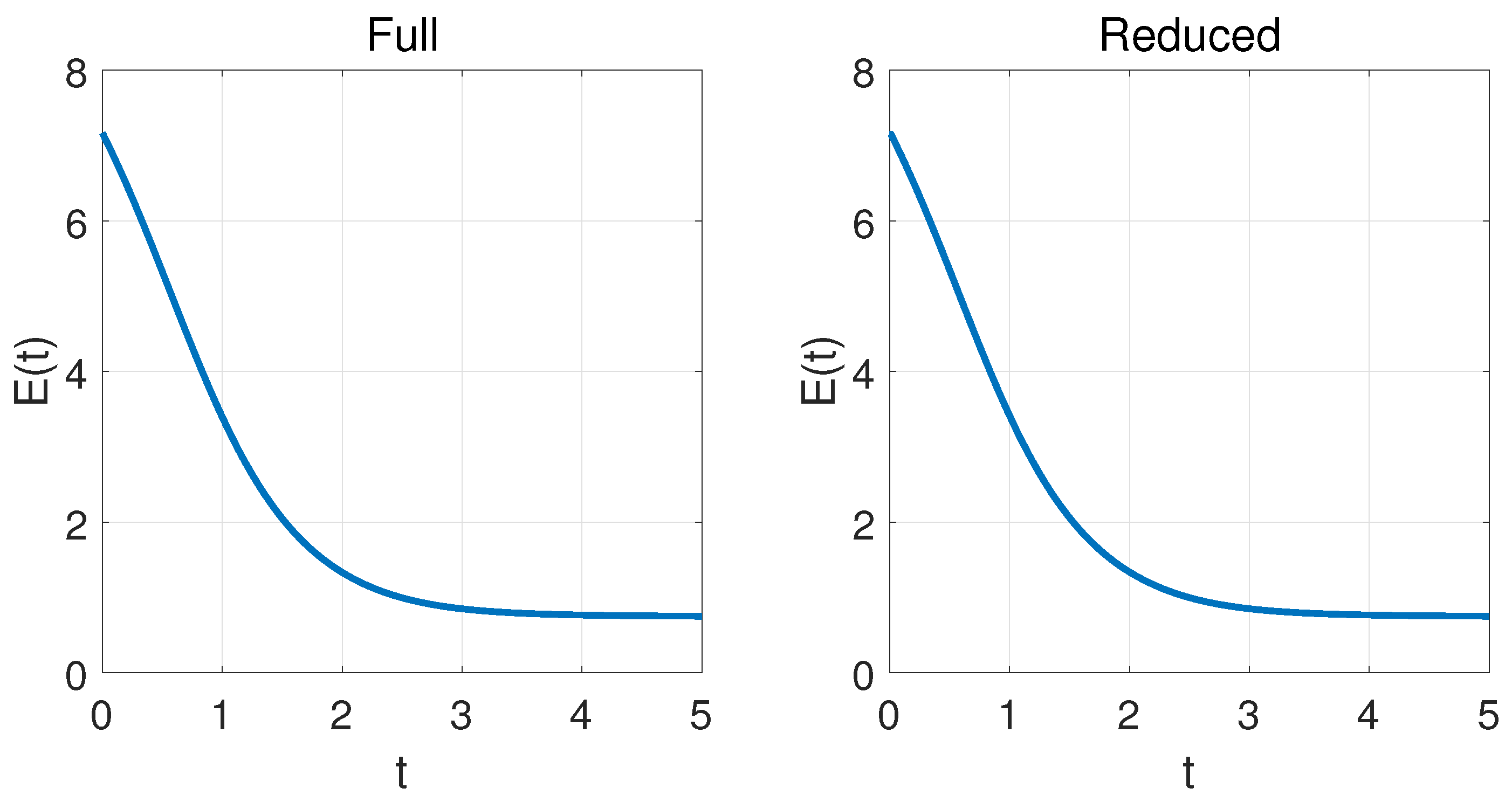
Figure 8.
3D AC: Energy plots (left) and radii of the spherical zero isosurface (right) by full/reduced solutions for .
Figure 8.
3D AC: Energy plots (left) and radii of the spherical zero isosurface (right) by full/reduced solutions for .
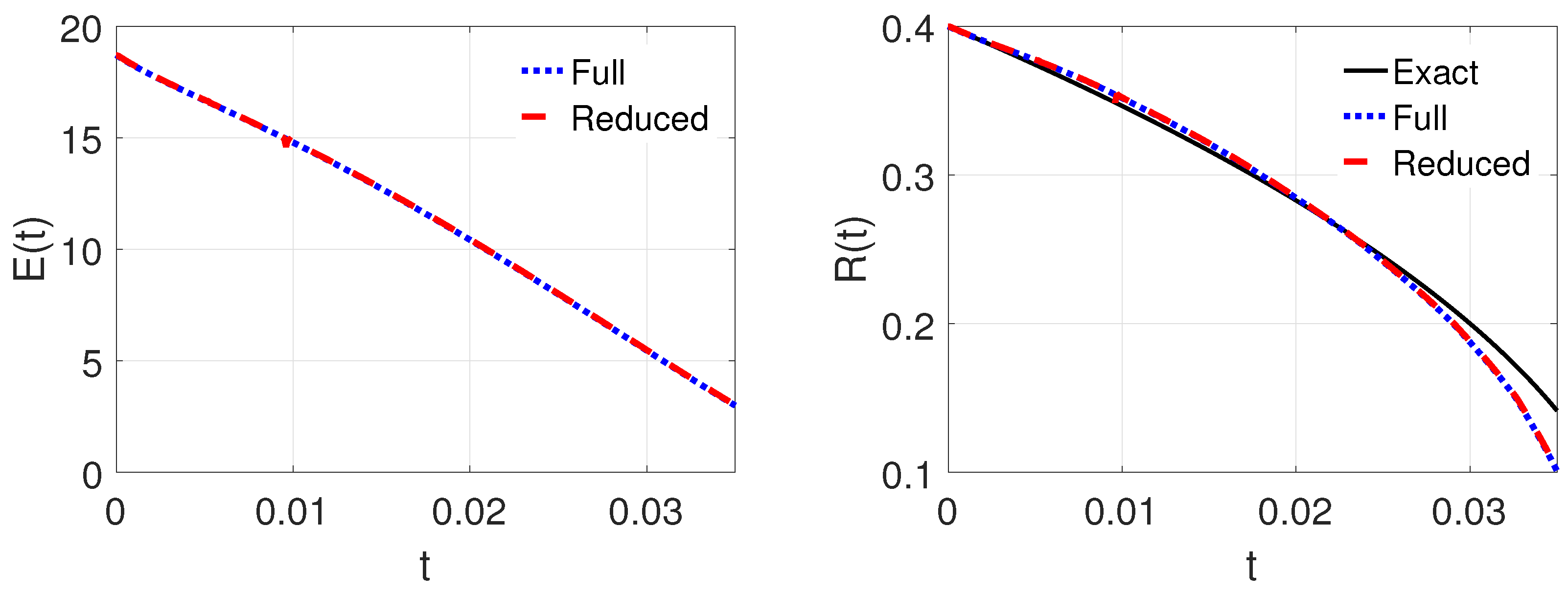
Figure 9.
3D AC: Snapshots of the zero isosurface of full (top) and reduced (bottom) solutions for .
Figure 9.
3D AC: Snapshots of the zero isosurface of full (top) and reduced (bottom) solutions for .
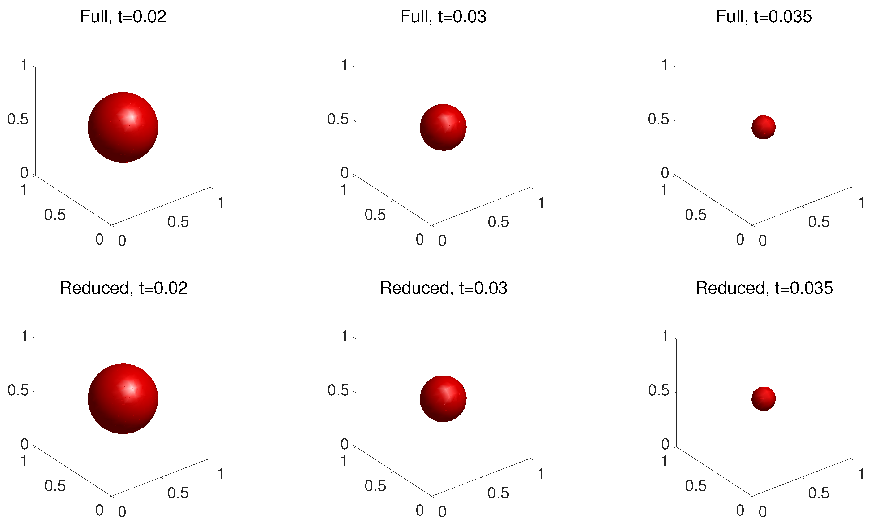

Table 1.
1D AC: Relative absolute errors for different values of k.
| k | 1 | 2 | 3 | 4 | 5 | 6 |
|---|---|---|---|---|---|---|
| PCA | 3.09e-01 | 1.28e-01 | 1.50e-02 | 1.55e-02 | 2.34e-03 | 2.41e-03 |
| KPCA | 2.56e-04 | 1.71e-05 | 1.88e-05 | 2.28e-04 | 2.71e-04 | 5.14e-04 |
Table 2.
1D AC: Relative absolute errors and CPU times for different values of k.
| Cpu Time (Sec.) | ||||
|---|---|---|---|---|
| With Iteration | Without Iteration | With Iteration | Without Iteration | |
| 1 | 2.56e-04 | 2.56e-04 | 3.7850 | 0.3690 |
| 2 | 1.71e-05 | 1.28e-04 | 3.9650 | 0.3800 |
| 3 | 1.88e-05 | 2.56e-04 | 4.2110 | 0.4115 |
| 4 | 2.28e-04 | 1.29e-04 | 4.0152 | 0.4025 |
| 5 | 2.71e-04 | 1.09e-03 | 4.6500 | 0.4780 |
| 6 | 5.14e-04 | 4.92e-03 | 4.7968 | 0.4975 |
Table 3.
2D AC: Relative absolute errors for different values of k.
| k | 1 | 2 | 3 | 4 | 5 | 6 |
|---|---|---|---|---|---|---|
| PCA | 2.80e-01 | 8.22e-02 | 4.78e-02 | 2.13e-02 | 6.53e-03 | 3.54e-03 |
| KPCA | 2.50e-03 | 1.49e-03 | 3.28e-03 | 1.92e-03 | 2.45e-03 | 1.37e-03 |
Table 4.
2D AC: Relative absolute errors and CPU times for different values of k.
| Cpu Time (Sec.) | ||||
|---|---|---|---|---|
| With Iteration | Without Iteration | With Iteration | Without Iteration | |
| 1 | 2.50e-03 | 3.80e-03 | 12.2090 | 1.4310 |
| 2 | 1.49e-03 | 1.89e-03 | 11.7000 | 1.6470 |
| 3 | 3.28e-03 | 3.77e-03 | 12.2340 | 1.5070 |
| 4 | 1.92e-03 | 1.82e-03 | 12.6700 | 1.7160 |
| 5 | 2.45e-03 | 3.66e-03 | 13.2030 | 1.8110 |
| 6 | 1.37e-03 | 1.68e-03 | 13.5700 | 1.8230 |
Table 5.
3D AC: Relative absolute errors for different values of k.
| k | 1 | 2 | 3 | 4 | 5 | 6 |
|---|---|---|---|---|---|---|
| PCA | 7.06e-02 | 8.55e-02 | 1.38e-02 | 1.16e-02 | 2.78e-03 | 4.85e-04 |
| KPCA | 4.57e-03 | 2.25e-03 | 4.83e-03 | 2.03e-03 | 6.68e-03 | 5.37e-03 |
Table 6.
3D AC: Relative absolute errors and CPU times for different values of k.
| Cpu Time (Sec.) | ||||
|---|---|---|---|---|
| With Iteration | Without Iteration | With Iteration | Without Iteration | |
| 1 | 4.57e-03 | 3.69e-03 | 12.2990 | 2.1780 |
| 2 | 2.25e-03 | 2.47e-03 | 13.4760 | 2.1510 |
| 3 | 4.83e-03 | 4.74e-03 | 14.1110 | 2.0270 |
| 4 | 2.03e-03 | 2.17e-03 | 14.1600 | 2.7510 |
| 5 | 6.68e-03 | 6.55e-03 | 15.2780 | 2.5950 |
| 6 | 5.37e-03 | 5.30e-03 | 15.1340 | 2.9640 |
Disclaimer/Publisher’s Note: The statements, opinions and data contained in all publications are solely those of the individual author(s) and contributor(s) and not of MDPI and/or the editor(s). MDPI and/or the editor(s) disclaim responsibility for any injury to people or property resulting from any ideas, methods, instructions or products referred to in the content. |
© 2024 by the authors. Licensee MDPI, Basel, Switzerland. This article is an open access article distributed under the terms and conditions of the Creative Commons Attribution (CC BY) license (http://creativecommons.org/licenses/by/4.0/).
Copyright: This open access article is published under a Creative Commons CC BY 4.0 license, which permit the free download, distribution, and reuse, provided that the author and preprint are cited in any reuse.


