
Submitted:
06 October 2024
Posted:
07 October 2024
You are already at the latest version
Abstract
The Lake Faro brackish basin (Sicily, Italy) was established Global Geosite as key locality of tectonic coastal lakes, but few were the research devoted this rare geological and ecological framework. To fill this gap, the main stratigraphical, sedimentological, ecological, morpho-bathymetric, and structural features were reported here first, linking geodiversity with biodiversity. In Lake Faro a shallow platform develops alongside a deep funnel–like shaped basin, reaching a maximum depth of 29 m. A NNW-SSE trending steep cliff, representing the abrupt transition from the platform to the basin, was interpreted as a dextral transtensive fault (Faro Lake Fault), presumably active since the late Pleistocene. The switches of the steep cliff NW-wards, acquiring a E-W trend, was interpreted as due to the occurrence of the Mortelle normal Fault, cut by the Faro Lake Fault. Abiotic bottom deposits consisted of coarse- to fine-grained quartzo–lithic rich sediments deriving from high grade metamorphic and igneous rocks, whereas the biotic component mainly consisted of bioclasts de-riving from clam farming actives for some centuries since today. The Quaternary shallow platform, from top to base includes: i) soft cover composed of coarse abiotic and prevalent biotic deposits; ii) hard conglomerates cemented by carbonates; iii) siliciclastic coarse deposits of the Messina Fm. In the deep basin, siliciclastic silty loams with minor amounts of biotic coarse deposits prevailed in the soft cover. The lake, exploited since the prehistoric age because of its high biodiversity and productivity, maintains some evidence of millennial relationships with the resident human cul-tures, there attracted by the favorable geomorphological and ecological peculiarities.
Keywords:
Coastal lakes
; Morpho-structures
; Geodiversity
; Biodiversity
1. Introduction
In the Cape Peloro coastal lagoon (CPCL, NE Sicily, Italy), two brackish basins, the Lake Faro (LF) and Lake Ganzirri (LG), fall down in two Global Geosites, denoted “Morpho–tectonic system of Cape Peloro–Lake Faro” and “Morpho–tectonic system of Cape Peloro–Lake Ganzirri”. Such sites also belong to a protected natural area, the oriented natural reserve of Cape Peloro, so that both geodiversity and biodiversity are protected. Recent geological and naturalistic investigations were carried out to provide their scientific inventory of the geoheritage and their quantitative assessment [1]. The research demonstrated that LF and LG are provided of high scores for the scientific value, the potential educational and the touristic uses (Figure 1). Indeed, the study morpho-structures resulted to be key localities, being developed on low-relief coasts because of Quaternary active faults [1].
Being these lakes key localities, showing indicators of representativeness, geological and biological diversity, and rarity, and considering the scarce literature devoted to this peculiar geological framework, the present research furtherly linked geodiversity with biodiversity, providing new insights on the LF shallow stratigraphy, sedimentology, and sedimentary petrography of the first meters of the soft cover bottom and substrate, and the related habitats, benthic biocenosis, and death assemblages, never analysed until now. Moreover, considering that the only existing data on the LF morpho-bathymetry go back to 1952 [2] an updated survey, using more advanced geophysical instrumentations, was also carried out. Structural investigations were finally realized, in order to detect macro- to mesoscale brittle deformation affecting the Cape Peloro peninsula to explain the origin of the LF morpho-structure.
2. Geological and Structural Framework
The CPCL is localized on the NE edge of the Peloritani Mountains, an Alpine Mountain chain, composed of a pile of seven thrust sheets and belonging to the Calabro-Peloritani Arc [3,4]. The basements consist of metamorphites affected by high– to low–grade Variscan metamorphism, locally intruded by late Variscan magmatic rocks, except for a few tectonic units [3,4,5,6,7]. Indeed, the Alì–Montagnareale Unit is formed only by a post–Varican succession affected by Alpine anchimetamorphism [8], whereas the Aspromonte and Mandanici Units are affected by an Alpine overprint [3,4]. Remnants of a Mesozoic-Cenozoic sedimentary covers cap some of these units [3,4] (Figure 2).
The Calabro-Peloritani Arc is localized in a seismically active region characterized by normal faults and raised Quaternary marine terraces recording the ongoing extension due to the southeastward rollback of the subduction zone [9].
Middle–upper Burdigalian thrust–top basins with siliciclastic sediments seal the tectonic units [3,4,10]. The post–orogenic uplift of the Peloritani Mountains improved a significative erosion of the basements and the sedimentation of siliciclastic successions [3,4,10] (Figure 2).
In particular, the Ionian slopes facing on the northern edge of the Messina Strait are made up of Pleistocene thick sequences [3]. These are constituted, from base to top, by: middle Pleistocene Messina Fm, upper Pleistocene Mortelle Fm, and upper Pleistocene Case Vento Fm [11,12]. The Messina Fm overlies in unconformity the high-grade crystalline basements and the Pliocene-Pleistocene deposits with thicknesses lower than about 250 m (Figure 2). It is composed of sands and gravels with well-rounded particles, deriving from metamorphic and igneous rocks, showing typical clinoforms with foresets dipping towards the central axis of the Strait of Messina [10,11,12]. The Fm, formed in fluvio-marine deltaic environment, shows at the base marine delta lithofacies (grey colored) overlain by continental-transitional deltaic lithofacies (red colored) [13,14,15]. On the base of the continental vertebrate contents, the age should not exceed 200±40 ky [14]. The Mortelle Fm. is formed by sands and silts with at the top intercalations of marls. The Fm is correlated with the Tyrrhenian terraces deposited in coastal lagoon environments connected with the sea, during a phase of incipient regression [10,11,12,13,14,15,16,17]. The Quaternary siliciclastic sequence ends with the Case Vento Fm that consists of sands and gravels of fluvio-marine Gilbert-type fan deltas followed by alluvial plain deposits [10,11,12,13,14,15].
Different orders of marine terraces, overlain by continental silts, sands, and gravels ranging between 236 and 60 ka, lie in unconformity on the siliciclastic Quaternary deposits. The origin of these terraces must be searched in tectonic phenomena and post- Würmian eustatic variations [3,10,11,12,13,14,15,16,17].
The most recent deposits of the CPCL are represented by Holocene coastal and alluvial siliciclastic deposits [18,19]. These sediments are mainly made up of sands and silts with intercalations of gravels, evolving downwards to gravels [20]. Peat intercalations may be present. Stratigraphic data on drilling cores indicate thicknesses ranging between 50-70 m in the Ganzirri-Torre Faro plain [3,17].
Along the shoreline, Holocene hard rocks are extensively exposed along a belt cropping out for tens of kms, from Mortelle (Tyrrhenian coast) throughout Cape Peloro up to Cape Ranieri (Port of Messina in the Ionian coast) [1,18,19,21,22]. These rocks, exposed when not covered by modern beach sands and gravels, are formed by very hard conglomerates with pebbles, cobbles, and boulders in a sandy matrix, cemented by carbonates [21,22]. These particles are composed of granitoids, porphyroids, and in general of high–grade metamorphic rocks, dating back to 6 ka B.P. [21]. Evidence of these hard rocks in the drilling cores carried out along the coast is lacking. On the base of the above, they are interpreted as beachrocks [21,22].
In the NE edge of the Peloritani Mountains, the Pleistocene-Holocene sediments developed in depocenters controlled by extensional structures connected both to the Tyrrhenian Sea opening and the collapse of the Ionian Sea [17]. The source area of the Fm, in the initial stages, was in the Tyrrhenian Sea, before its collapse because of the activity of E-W trending normal faults. Normal and strike-slip faults sometimes may also cut the actual deposits on the sea bottom [17,20,23].
The landscape was shaped by a complex network of faults responsible for the origin of tilted blocks, horst and demi–horst morpho–structures (as the Ganzirri horst [11,12]) onshore, and graben and demi-graben morpho–structures offshore, as revealed by seismic reflection profiles carried out in the Messina Strait Sea bottom [23]. In particular, the main complex array of macroscale faults affecting the Sicilian slope of the Messina Strait may be brought back to the following main fault systems [24]:
- The E-W trending fault system, denoted Mortelle Fault System [24].
- The NNE–SSW trending fault system (about 15 main macroscale faults denoted n. 45-60 in [24]), denoted Messina or Messina-Taormina Fault System.
- The NW-SE to NNW-SSE trending fault system (about eight main macroscale faults denoted n. 61, 62, 64, 65, 66 or without number [24], denoted Faro Superiore or Curcuraci Fault System.
- The ENE–WSW trending fault system [about two main macroscale faults denoted n. 63, 66 in [24], denoted Scilla Ganzirri or Ganzirri Fault System.
The fault systems were ascribed to extensional tectonics, except the NW-SE to NNW-SSE trending faults (FSFS) characterized by an oblique transtensive displacement with a right lateral component, as reported in several structural and seismotectonic maps of the NE Sicily [11,12,24,25,26]. These latter were considered right lateral transtensional faults. A transtensional displacement was also confirmed by structural mesoscale data recorded by the authors in the Tindari area (unpublished data) (Figure 3). Physical evidence for the ENE–WSW trending macroscale normal faults is reported on onshore seismic profiles [27,28,29].
The valuable results of a geomorphological and structural research on the modification of the hydrographic network of the Ionian Sicilian slope of the Messina Strait suggested that the WSW-trending drainage system developed in the Late Pleistocene (90–100 ky), as a consequence of the activity of the Faro Superiore or Curcuraci Fault System, whereas the successive drainage system shifted to NNW-SSE trends, developed in the Tyrrhenian as a consequence of the activity of the Scilla-Ganzirri Fault System, actually controlling the present-day trend of the Ionian coast in the northern edge of the Messina Strait [18], being Quaternary active faults.
3. The Cape Peloro Coastal Lagoon (CPCL)
The CPCL extends in the north-eastern edge of the Peloritani Mountains, in an area covering about 68.12 hectares comprised among the Torre Faro and Ganzirri fisher villages (Messina, Figure 4), in the Cape Peloro peninsula. The lagoon faces both in the Tyrrhenian and Ionian Sea and hosts two brackish basins, denoted Lake Ganzirri (LG) and Lake Faro (LF).
Both basins are located in a crucial protected area, the oriented natural reserve of Cape Peloro (Figure 5a,b), established since 2015. The lagoon was also declared Site of Community Importance and Special Protection Zone, according to the European Directives, for its important bioheritage, being a unique brackish environment where the vegetation represents a sanctuary for migratory birds. The lagoon was also stated as "Heritage of ethnic–anthropological interest", because of traditional mussels, clams, and cockles farming [1].
Moreover, the protected area hosts two geosites, known as "Morpho–tectonic system of Cape Peloro – Lake Faro" and "Morpho–tectonic system of Cape Peloro – Lake Ganzirri" (Figure 5b). These two geosites were introduced in April 2015 in the list of the about one hundred geosites established by the Sicilian Region. The geodiversity preserved in the lakes is provided of high scientific value for its peculiar morpho-tectonic origin at the global scale [1].
4. The Lake Faro (LF)
The LF is a small brackish coastal lake showing a peculiar sub–circular shape, covering an area of about 263,600 m2 (Figure 6). The maximum length (ENE–WSW) and width (N–S) are 600 m and 562 m, respectively. The boundary of the lake is entirely anthropized, being mostly delimited by cemented ramps, streets, and small buildings facing directly to the lake. The lake is lightly connected to the Ionian Sea through an artificial canal (Canal Faro), about 8 m wide and 425 m long, opening in the Strait of Messina. During the summer, an artificial connection with the Tyrrhenian Sea (Canal degli Inglesi, about 8–10 m wide and 182 m long) is occasionally opened for receiving marine waters, to improve the water chemical–physical quality of the lagoon, thus indirectly favoring the local mussel farming activities. Other indirect connections with the sea occur through the Canal Margi (about 8–12 m wide and 904 m long), connecting the SW side of LF with the close LG, on its turn connected with the Ionian Sea through the Canal Due Torri (about 10 m wide and 302 m long) [1].
4.1. Origin of the Lagoon
Two main contrasting hypotheses were proposed in the past for interpreting the origin of the lagoon.
Segre et al. [21] explained the origin of the deep-seated funnel–shape of LF, as depending exclusively on geomorphological phenomena, occurred during the Late Pleistocene –Holocene time span, related to cold currents causing a deep whirl excavation (Figure 7a) of the sea bottom in front of the Faro–Pelorus headland. The E–wards littoral warm currents (Figure 7b), occurring after the previous cold paleocurrents, after the Pleistocene–Holocene transition, determined the formation of a littoral sand bar shoal external to the paleo Lake Faro (Figure 7b), lying on flat sea floor made up of pebbles and conglomerates. Finally, this littoral warm current circulation became stable about 11,000–9,000 years B.P. [21] (Figure 7c).
It is noteworthy that the depressions hosting the lagoon with its costal lakes developed because of the post-orogenic strong extensional tectonics [1] and the subsequent post–Würmian sea–level rise. First authors to infer a tectonic origin to the LF were, in 1953, Abbruzzese and Genovese [2]. Half a century later, Bottari et al. [22] confirmed a tectonic evolution for both CPCL lakes. In particular, the authors showed the results of geological and geophysical surveys. Indeed, an ENE-WSW trending normal fault, the Ganzirri fault, at the base of the hills and bordering the NNW side of LG, was identified in high resolution seismic profile SM-02 and SM-07 and interpreted as the responsible for the formation of the LG [22,27,28]. The fault system was responsible for creating a horst like morpho-structure, onshore in the hills of Cape Peloro, contraposed to down thrown fault hanging walls in the Ionian coast and the Messina Strait. After the above-mentioned research and the study of Bottari and Carveni [29], describing the occurrence of an ancient port and depicting a morphological reconstruction of the lagoon, no further structural or geophysical investigations were devoted to the CPCL lakes.
Analyzing the main trends of structural data reported in the major CPCL geological-structural sketch maps [11,12,24,25,26,30] at least three main fault systems may be recognized. The main macroscale fault systems shaping this landscape are:
- i.
- The E-W trending (N-dipping) normal faults, denoted Mortelle fault system.
- ii.
- The NNW-SSE to NW-SE trending (ENE–to NE-dipping) extensional faults with a dextral strike-slip component.
- iii.
- The ENE–WSW trending (SSE–dipping) normal faults.
4.2. Ecological Framework
Literature data indicated LF as a limno–lagoonar basin [21] with a peculiar meromictic regime that has drawn the attention of specialists at an international level. The above cited peculiarity is tied to the funnel–shaped floor that, hindering the water mixing, separate an upper oxygenated mixolimnion layer, rarely exceeding 15 m depth, from an equally thick sulfide rich anoxic monimolimnion. The remaining shallow lake floors, affected only by the mixolimnion layer, generally does not suffer of oxygen depletion, except for the 3.5 m depth small depression, not shown in the historical maps, that is characterized by persistent hypoxic conditions [31].
Surface waters are mesotrophic, and seasonal blooms generally do not cause dystrophic crises [32,33]. However, in the past, wider than now seasonal changes in the monimolimnion extent occasionally affected the surface waters, causing water acidification and anoxic crises [34]. As expected in a brackish basin, environmental parameters are subject to marked seasonal and interannual variability. Surface water temperatures range from 13.80 to 29.43°C, with the lowest temperature of 10°C in February and the highest of 29°C in August. Salinity values range from 26.5 to 38.6, and the oxygen concentration in surface waters ranges from 73.82 ± 3.40 % to 92.55 ± 7.53 % [35,36].
Despite the weak connection with the sea, the mixolimnion is remarkably influenced by the Messina Strait tidal regime and related upwelling, as proved by Saccà et al. [35] which found evidence of sporadic inputs of Levantine Intermediate Waters (LIW) in LF picoplankton communities. Due to the meromictic regime and close biological implications, microbiological investigations have been carried out since Genovese [37], and LF proposed as model under several aspects (e.g. [38,39]). Similarly, the plankton communities have provided case studies at different levels of investigations (e.g. [40,41,42,43]).
The high urbanization of the surrounding area did not hamper that most original features have been preserved, although requiring continuous protection and enhancement. Among the irremediably lost habitats, the disappearance of a vast area used as salt pans, in relatively recent times (early 20th century), is emblematic. The salt pans reclamation, depriving the brackish area of a relevant and peculiar portion, notably impoverished the whole lagoon system, both in structural, ecological, ethnoanthropological and cultural heritage.
Tied to the notable anthropogenic pressure, some evidence of chemical (e.g. [44]) and biological contamination (e.g. [45]) have been reported in the past. Mussel and oyster farming (e.g. [46]) are major responsible of frequent introductions of not indigenous species (e.g. [46,47]).
Although the high naturalistic and ecological value of this brackish area is evident, it has been scarcely documented in the past, by few scientific papers, concerning avifauna (e.g. [48]) and macrophytes (e.g. [49,50]). Aquatic invertebrates have been mostly reported in recent years, revealing high biodiversity (e.g. [51,52]), but also a long-term decline of relevant taxa, as the mollusks [53]. Some poorly known (e.g. [54]) and endemic species (e.g. [55]) have been also reported. By contrast, the role of LF as steppingstone facilitating the spreading of marine alien species has been underlined [46,47].
Currently, the most relevant aspect is given by the persistence of a residual population of the threatened bivalve Pinna nobilis (Figure), which makes the LF one of the latest sanctuaries of this habitat forming species at risk of extinction (e.g. [31,56]).
As far as concerns the characterization of the main benthic habitats, preliminary data on the occurrence of rhodolith beds were given in [57].
5. Materials and Methods
Investigations aimed to reconstruct the morpho-bathymetry of the bottom, as well as investigate the brittle deformation, texture, and petrographic composition of the sediments, and the main habitat typologies of the LF, were carried out. The bathymetric instruments and surveying equipment belong to Metralab srl (Padova), whereas the laboratory instrumentations and sampling equipment used for geological and biological investigations belong to the laboratories of geology, forensic geology, and benthic ecology of the University of Messina.
5.1. Sampling Activities and Laboratory Analyses
The soft lacustrine cover and the hard substrate of LF were investigated. Six samples of shallow and deep soft deposits were collected by means of manual sediment core sampler used during snorkeling and SCUBA activities and of a van Veen grab sampler (400 cm2 surface) used from a traditional fisher boat, respectively. The thickness of the shallow lacustrine cover was measured by means of a graduated metal T–bar. Two samples of hard substrate were also collected.
5.2. Morpho–Bathymetric Reconstruction
In the LF environmental context, bathymetric measurement with a single–beam ultrasound device was considered the most efficient approach. The employment of more expensive tools, as multi–beam echo sonar or laser sonar for measurement, in fact, would not have been significantly compensated for by higher resolution, due to the high disturbance caused by the patchy distributed shallowest lake floors, and by the numerous sources of lateral reflection, especially scattered anthropic structures. To comply with the recommendations of the International Hydrographic Organization (IHO) [58] regarding frontal waves, a traditional fishing boat was selected. The boat was chosen for its compact dimensions, cost–effective engine, and ease installation of surveying equipment and instruments.
The bathymetric measurement was carried out using an integrated measuring system. The installed equipment comprised a HydroStar 4300 sonar and GNSS devices Topcon HyPer Pro, enabling real–time connection and data registration. This setup facilitated the recording of sonar coordinates and corresponding depth. The software Surfer automatically converted the GPS coordinates into the local projection coordinates, with the chosen projection being WGS84DD.
The bathymetric survey adhered to pre–established profiles on a geo–referenced cartographic surface. The planned survey profiles ensured comprehensive coverage and high resolution in the research area. Additionally, some transversal profiles were incorporated to intersect with the main profiles, enabling comparison and control of the measured depths. A total of forthy measure transects, oriented N-S and E-W, with a spacing of about 15 m, were carried out.
5.3. Habitat
A visual monitoring of the whole shallow lake bottom (< 2 m depth) was carried out by snorkeling. Moreover, SCUBA observations were carried out deeper than 2 m depth, up to 15 m depth in the deepest portion of the lake. Main abiotic and biotic features of the lake floor were directly reported on field-tablets and photo and/or video documented.
Samples of biogenic bottom deposits, as well as specimens of living benthic fauna were manually collected. All main habitat typologies were localized by using a GPS.
5.4. Textural Features
Particle size analyses (PSA) of the modern lake sediments were conducted in soft samples.
The analyses of the coarse grain sizes (gravels and sands) were performed using a mechanical siever (AS 200 control model, Retsch, Düsseldorf, Germany) with sieves provided of the following opens: -1, 0, 1, 2, 3, 4 phi [-log 2 d(mm)]. Additional sieves were used for the analysis of gravelly sands (-4.2, -3.6, -3.2, -2.7, -2.2, -2.0 phi). Due to the significative presence of mud, samples were sieved in wet conditions.
The analyses of the fine grain sizes (silts and clays) [< 4 phi (62.5 µm)], after treatment with sodium hexametaphosphate, were performed by means of a diffraction particle size analyser in wet conditions. The instrument was a laser diffraction particle size analyser (Mastersizer 2000, Malvern Panalytical Ltd, Malvern, UK) able to measure particle in the size range 0.02–2,000 µm. PSA data were expressed in frequency and cumulative per cent curves. The statistical parameters (mode, inclusive mean, kurtosis, skewness, sorting) were automatically provided by the system Mastersizer 2000.
PSA data of coarse to fine particles were finally expressed in cumulative per cent curves and the statistical parameters automatically calculated by means of the software Gradisat.
The texture of the hard rocks was analysed at mesoscale and in polished surfaces realized by precision rock cutting.
5.5. Petrographic Composition
The petrofacies were analysed by means of optical microscopy (OM) under stereomicroscope and petrographic microscope. Thin sections of sands with very coarse grains, aggregated in epoxy resin were carried out.
The instruments used for OM were a motorized stereomicroscope with reflected and transmitted polarized light (Zeiss Stereo Discovery.V20, magnification from 3.8x to 530x with optical zoom) and a motorized petrographic optical microscope with reflected and transmitted polarized light (Zeiss Imager.M2m model, magnifications from 25x to 500x). Both microscopes were coupled to telecamera and workstation using image analysis software (Axiovision, Carl Zeiss AG, Feldbach, Switzerland).
Preliminary mesoscale petrographic observations were carried out also in the underlying hard substrate. A visual mesoscale inspection was devoted to pebbles and cobbles in order to characterize their mesoscale petrographic features by means of eye lens. Due to their evident compositions, textures, and structures, most of these materials were easily classifiable.
5.6. Structural Geology Analysis
In zones at high seismic risk (zone one, INGV), as the Calabria-Peloritani Arc, seismogenic faults and fault zones may be detected identifying the related earthquake sources or acquiring data from geological-structural surveys and geophysical prospections.
Field and satellite imagery observations at macroscale and mesoscale structural investigations were carried out for establishing the presence of active faults at different scale in the most recent deposits. Each workstation was localized by GPS.
6. Results
6.1. Morpho–Bathymetric Reconstruction of LF
The morpho–bathymetric survey allowed depicting two main landforms, consisting of a shallow platform at west and a peculiar deep funnel–like shaped floor at east. This depression shows a maximum depth at - 29 m isobath and its shape is mostly N-S switching, in its NW edge, in a E–W orientation. The shallow platform is sub–horizontal and gently dipping E-wards with depths not exceeding the - 2 m isobath, except in a weak NNW–SSE trending small depression, reaching - 3.5 m depth (Figure 8). The slope bounding the eastern side of the platform is provided of steep inclination.
6.2. Sampling Activity
Six samples of the lacustrine soft cover were collected at few cm of depth on the lake bottom, along an E-W trending transect crossing the platform and the deep funnel–like shaped floor, from West to East, respectively (Figure 9, Table 1). The samples F45-44-46 were collected on the platform. The samples F138-149 were taken on the deep depression. The sample F41 was collected on the western slope of the lake. Two samples of hard conglomerates were collected along the cliff border (Figure 9, Table 1).
6.3. Stratigraphical and Sedimentological Data on the LF
A modern lacustrine soft cover was identified on the lake bottom from the platform to the deep funnel–like shaped floor. The typical blackish color of most of these deposits suggested high amounts of organic matter. The thickness of the lacustrine cover is about 1.5-2 m on the LF shallow platform, whereas along the cliff border it is only a few centimeters thick or absent due to occasional gravitative slumps.
On the plattform, these deposits appear artificially and intensively reworked on the lake bottom, being their composition altered by all sorts of anthropogenic materials. Indeed, the lake bottom underwent remarkable anthropogenic alterations due to clam farming activity. The anthropogenic origin of most of the lacustrine cover is testified by the presence of coarse material composed of entire or fragmentated shells (bivalves and gastropods), due to the shellfish farming activities.
The biotic coarse material prevails on the platform, being very low the amount of fine siliciclastic sediments, whereas the fine fractions prevail on the deep funnel–like shaped floor, being low the amounts of biogenic particles.
The lacustrine soft cover overlies a natural hard substrate present along the scarp bounding the eastern side of the platform. The substrate, at least 2 m thick, is well observable along the scarp at about 4 m of depth. It consists of conglomerates deeply cemented by carbonates.
The cemented conglomerates overly the gravels and sands of the Middle Pleistocene Messina Fm exposed along the steep cliff, when not overlain by shallow deposits. The Messina Fm is also the substrate of the deep funnel–like shaped floor, on turn covered by a layer of various thickness and consistency. A thick nepheloid layer, moreover, widely occurs.
The survey of the stratigraphic boundaries among the soft cover, the hard conglomerates and the Messina Fm is still in progress, due to the complexity associated with SCUBA activities in identifying them.
6.4. Habitats and Ecosystem Asset
The shell-rich soft cover is colonized by encrusting red algae, frequently forming rhodolith beds (Figure 10a).
Stable patches of the seagrass Cymodocea nodosa, colonizing both the shell-rich soft cover and the siliciclastic sands, have been first reported in the north-western lake borderline and inner part of the canal Faro, respectively (Figure 10b). Similarly, a wide natural hard rocky substrate (made up of conglomerates) with relevant sessile communities, rising througout the shallow platform and the boundary of the steep cliff, has been first reported (Figure 10c).
As an effect of long-time anthropogenic modification of the native habitat, the artificial “sandy mounds” used for clam farming, need to be mentioned. Mostly mounds, whose distribution agrees with the cadastral parcels given under concession (Figure 6), are abandoned, and highly colonized by a rich soft bottom fauna (Figure 10d). Moreover, where the wave action removed the mound covering, remnants of artificial hard bases of the mounds, made up of bricks and blocks, emerged, providing an available substrate for flourishing hard-bottom communities (Figure 10e).
However, the most peculiar and large habitat in the LF, extending approximately from -12 m to the maximum depth of the basin, at -29 m, is characterized by anoxic and H2S rich waters. Due to the anoxic conditions, only microbial communities occur but producing a so high biomass that the resulting bacterial mats are responsible for a varied and impressive underwater landscape (Figure 10f).
6.5. Benthic Biocenosis and Death Assemblages
According to the Pérès & Picard model, a generic “Euryhaline and Eurythermal Lagoon biocenosis” can be recognized in the innermost areas, while most lake-floors are characterized by the “Superficial Muddy Sand in Sheltered Areas biocenosis”. Instead, according to the Barcelona Convention classification, updated to 2013 [60], the following associations belonging to the “habitats of transitional waters” have been detected:
MB1.541 Association with marine angiosperms or other halophytes;
- i.
- MB1.542 Association with Fucales;
- ii.
- MB5.543 Association with photophilic algae (except Fucales);
- iii.
- MB5.544 Facies with Polychaeta;
- iv.
- MB5.545 Facies with Bivalvia.
Inside such associations, a combination of marine and brakish species occurred, resulting in a high grade of biodiversity.
Several non-native species have been also recorded, generally tied to the non-intentional introduction of opportunistic colonizers, througout the inport, stabling and farming of shelled edible molluscs. Between such non-native species, the ascidian Styela plicata Lesueur, 1823 and some annelids as Branchiomma luctuosum Grube, 1870 and Branchiomma boholense Grube, 1878 need to be cited for their extreme invasiveness. By contrast, the settlement of non-indigenous molluscs, as the mussel Brachidontes pharaonis Fischer, 1870 and the arc clam Anadara transversa Say, 1822, did not determine evident ecosystem imbalance.
By contrast, the persistence of some exclusive endemic taxa, as the annelid Myxicola cosentini [56], and the gastropod Tritia tinei Maravigna, 1840, is underlined, as a prove of an ancient genesis of the LF basin.
Death assemblages from the six surface-subsurface soft cover samples provided a high amount of data about the actual and subactual mollusc fauna, with evidence of changes occurred in hystorical times. Most recent deposits, indeed, are characterized by large amount of shells resulting from the stabling of non-native bivalves, as the “cock”, Callista chione Linnaeus, 1758, and the “portuguese oyster, Magallana gigas Thunberg, 1793. Due to the disomogeneous anthropogenic impact, patch distributed deposits of less recent age have also recognized, being characterized by some species no more found as living nowadays in LF. Some of these, as flat sunsetclam, Gari depressa Pennant, 1777, are characteristic of coarse deposits and well oxygenated waters. Other species, as the brittle cockleshell, Gastrana fragilis Linnaeus, 1758, are generally associated with marine angiosperms or other halophytes in sheltered environments. Moreover, the gastropod Pirenella conica Blainville, 1829, known from extreme brachisk basins, as the salt pans, has been sporadically recorded. Notably, all the P. conica specimens showed the peculiar smoth ornamentation and brown colour reported for the alleged endemic Cerithium peloritanum Cantraine, 1835, now synonimized with P. conica. Rarely, partially diagenized shells of the flat oyster, Ostrea edulis Linnaeus, 1758, testified about the ancient occurrence of this important edible species.
At last, sediment samples collected in the deepest anoxic zone (F138-149) provided a fraction of coarse bioclasts mostly recognizable as shell remains of both species of farmed mussels, Mytilus edulis Linnaeus, 1758 and M. galloprovincialis Lamarck, 1819, related with the overlying long-lines cultures. The same tools are responsible of the release of the abundant sponge silicatic spicoles found in the silty fraction at -28 m depth (sample F138).
6.6. Textural Data
Six samples of soft coarse- to fine-grain cover (F45-44-46-138-149-41) were analysed, as it was, by means of mechanical sieving (in wet conditions; Table 2).
The soft cover, collected on the platform, consisted of coarse abiotic and biotic deposits with very low percentages of mud. Sample F44 was mainly formed by siliciclastic sandy gravels with a minor amount of clam farming bioclasts in the size fraction < 125 µm (observed under stereomicroscope). Differently, samples F45-46 were made up of clam farming bioclasts in the range between gravelly sands and gravels with sands, prevailing on the abiotic component in the size fraction < 63 µm. Samples F45-46 may be classified as “shell-rich coarse deposits” on the base of the size of the biotic remains (Table 2).
The soft cover, collected on the deep funnel–like shaped floor (F138-149), consisted of siliciclastic muds pevailing on a biotic sand/gravel component of clam farming bioclasts in the size fraction > 63 µm (observed under stereomicroscope).
The soft cover, collected on the western slope of the lake, consisted of abiotic deposits with very low mud. Indeed, sample F41 was mainly formed by siliciclastic gravelly sands with a minor amount of clam farming bioclasts.
Biotic carbonatic traces were found togheter with the finest mineral matrix in all the samples.
PSA data by laser diffraction on the fraction with size < 63 µm of the soft cover indicated that the fine material mainly consisted of silty loams (F45-44-46-138-149-41). The texture was characterized by low sorting (poorly sorted), fine skewness (rarely symmetrical), and mesokurtic values (rarely platykurtic) (Table 3, Figure 11).
The mesoscopic observations on the polished sections of the two samples of hard conglomerates (FHC01, FHC02; Table1, Figure 9), made also under stereomicroscope, allowed to identify clast-supported conglomerates with very well rounded pebbles with minor cobbles in a sandy matrix, deeply cemented by carbonates (Figure 12).
6.7. Petrographic Data
The mineral sandy to silty particles present in the soft cover (samples: F41, F44, F45A, F46, F138, F149) were observed by visual inspections and analysed by OM observations under stereomicroscope and petrographic microscope. Stereoscopic observations indicated that particles were mainly composed of monomineral siliciclastic grains showing typical features compatible with hyaline quartz, white feldspars, and micas (biotite prevailing), with polycristalline grains mostly composed of quartz+biotite, quartz+muscovite, and quartz+feldspar paragenesis (lithoclasts of gneiss and granitoids). The same samples, analysed under petrographic microscope resulted to be quartzo–lithic rich sediments, being composed of metamorphic monomineral quartz, plagioclase, biotite grains (50%, Figure 13) and metamorphic lithics (50%) mainly made up of quartz+plagioclase, quartz+biotite, quartz+muscovite mineral paragenesis (Figure 13). Peculiar microstructures were recognized in the quartz grains, being pervasively deformed with different joint systems (Figure 13).
The hard conglomerates resulted to be composed of particles of cristalline rocks (high grade metamorphic and igneous rocks) in a quartz prevailing sandy matrix, deeply cemented by carbonates (Figure 12).
6.8. Structural Geology Data
Macroscale field and remote sensing observations were carried out in the study area.
In the Torre Faro-Granatari area, a macroscale fault scarp, bounding the LF and still reported in the literature (normal fault n. 62 in [25]) at the base of the hill, appears with NNW-SSE/NW-SE trend and ENE dip (Figure 14).
Parallel to this fault, eastwards, another macroscale structural element was detected underwater in the lake. Indeed, analogously, it resulted to be mostly NNW-SSE trending and with ENE dip, and NW-wards E-W oriented. This surface was better observed during the morpho-bathymetric survey and subaqueous snorkeling and SCUBA activities. This fault appeared along the lake platform steep cliff, developing among -2 m and -29 m isobaths, mostly overlain by the soft cover (Figure 14).
Mesoscale deformation was also searched in the sands and gravels of the middle Pleistocene Messina Formation, representing these deposits the substrate of the LF, the CPCP in general, and the main formation exposed in the hills surrounding the plain affected by macroscale faults. Tens of mesoscale faults, notwithstanding the difficulty to detect deformations in incoherent sediments, were identified (Figure 15). These structures, never detected until now, were characterized on the base of the fault kinematic indicators and the stratigraphic features showed by the fault hanging walls and footwalls. The main indicators consisted in small cm-sized drag folds allowing to recognize normal type faults. The entity of the displacement was at cm-scale, reaching about 15 cm. The main structural trends of the study mesoscale faults were ENE–WSW, from NNW-SSE to NW-SE, and E-W. The faults resulted to be normal faults except the NNW-SSE faults being characterized by dextral transtensive displacements (Figure 15).
The mesoscale data on the NNW-SSE trending faults allow to better characterize the macrofaults recognized on the LF area. These are the evidence of the tectonic origin of the funnel-shaped depression. The morpho-tectonic structure identified on the LF could represent a tilted block, dominated by transtensive dextral displacements (Figure 16a). Figure 16 illustrates in sketch maps the main macroscale faults affecting the Cape Peloro peninsula, reporting them on topographic surfaces elaborated in [29] with different elevations on the sea level (Figure 16a,b; [29] modified).
7. Discussion and Concluding Remarks
7.1. Geological Evidence in the Framework of the Northernmost end of the Messina Strait
7.1.1. Stratigraphic Framework
The general Quaternary stratigraphic framework, here first described, was characterized by two different successions.
The lithostratigraphic succession reconstructed in the shallow platform consisted, from top to base, of:
- i.
- Soft cover formed by coarse abiotic (siliciclastic sandy gravels) and shell-rich deposits (gravelly sands to gravels with sands), the latter prevailing on the first ones (about 1.5-2 m thick).
- ii.
- Hard conglomerates cemented by carbonates (at least a few meter thicks).
- iii.
- Sands and gravels of the Messina Fm (middle Pleistocene).
The coarse abiotic and biotic deposits of the soft cover present in the platform showed a very low percentages of mud (silty loams) with biotic carbonatic traces, ranging from 0.06 to 5% (Table 2). The shell-rich deposits, found from coarse to the fine materials, derived from the ancient clam farming tradition present still today.
In the slopes and deep funnel–like shaped floor, it was only possible to characterize the first soft cover, presumably lying on the Messina Fm (middle Pleistocene), due to the elevated risks for the SCUBA divers operating in dark waters with numerous obstacles of anthropogenic orygin. Deep samples consisted of muds (silty loams) with minor amounts of shell-rich gravelly sands and gravels with sands.
The silty loams, found on the shallow and deep environments, were mainly provided of low sorting, fine skewness, and mesokurtic values (Table 3, Figure 11).
In most of the study samples, the percentage of sands made up of clam farming bioclasts appeared to decrease from west to east, along a transect realized from the platform to the deep funnel–like shaped floor (Table 2, Figure 9). Indeed, the percentage of shell remains of the soft cover decreased from 82% in the platform up to the 19% on the deepest areas. Conversely, the amounts of silty loams appeared to increase from the platform to the deep funnel–like shaped floor (Table 2, Figure 9).
The abiotic component of the soft cover resulted to be formed of pebbles of high grade metamorphic and igneous rocks. Analogously, the siliciclastic sandy to silty particles resulted to be quartzo–lithic rich sediments (particles of metamorphic quartz, plagioclase, biotite, quartz+plagioclase, quartz+biotite, quartz+muscovite, Figure 13). Source rocks of these sediments have been recognized in the granitoids and high–grade metamorphic basements of the Aspromonte Unit and the underlying Messina Fm. responsible for nourishing the alluvial and coastal plain of the Cape Peloro peninsula. Indeed, the composition of the LF deposits resulted to be similar to that recently analysed in the Tyrrhenian and Ionian beaches of the peninsula [19].
The hard conglomerates resulted to be clast-supported and composed of pebbles with cobbles in a sandy matrix, deeply cemented by carbonates (Figure 12). The particles were formed of high grade metamorphic and igneous rocks. The results of a research devoted to composition, texture, and structure and structural investigations on these conglomerates, together with comparison with the analogous Holocene beachrocks bounding the Tyrrhenian and Ionian marine coast of the Cape Peloro peninsula, are still in progress and will provide in the next future.
7.1.2. Morpho–Bathymetric and Structural Geology Framework
The recent morpho–bathymetric survey, carried out by means of a single–beam ultrasound system, here first described, allowed to define the shape and aspect of the LF bottom at high resolution. Indeed, the survey data, further to depict a deep funnel–like shaped floor (maximum depth at - 29 m), bouded along a steep cliff, by a shallow platform at west (maximum depth at - 2 m), as previously recognized by Genovese and Abbruzzese [2] allowed to better investigate the platform shape, evidencing the occurrence of a depression parallel to the cliff, in the SW side (Figure 8c,d). The steep cliff showed a NNW-SSE trend switching NW-wards in a E-W trend.
In the Torre Faro-Granatari-LF area, macroscale fault scarps were detected. A fault with NNW-SSE/NW-SE trend and ENE dip (Figure 14) bounds the LF at the base of the hill. Parallel to this scarp, eastwards, another fault scarp may be identified in the steep cliff bounding the eastern side of the LF platform. The fault, mostly NNW-SSE trending, NW-wards switches to E-W. The NNW-SSE surface was better observed during the morpho-bathymetric survey and subaqueous snorkeling and SCUBA activities, developing among -2 m and -29 m isobaths, mostly overlain by the soft cover (Figure 14). Mesoscale structural investigations carried out in the middle Pleistocene Messina Fm, being these deposits the substrate of the LF, revealed for the first time the presence of tens of mesoscale faults, parallel to the main macroscale fault system affecting the northern edge of the Messina Strait area (Figure 3). Kinematic indicators were typical of normal type faults, except along the NNW-SSE faults, being characterized by dextral transtensive displacements as in the Faro superiore or Curcuraci fault system.
Considering the previous hypotheses for interpreting the origin of the LF [21,22], the data here reported should suggest a tectonic genesis for the LF, dominated by en-echelon system of NNW-SSE dextral transtensive faults (Faro Superiore or Curcuraci fault system; Figure 16). These Quaternary faults, presumably active since the late Pleistocene, may belong to an active conjugate relay zone where the displacements on the strike-slip faults are transferred to the Messina-Taormina normal fault system within the Messina Strait framework [9].
In the northernmost edge of the Messina Strait, about 11,000–9,000 years B.P., stable E-wards littoral warm currents dominated in the Tyrrhenian Sea and the paleolake Faro was presumably linked to the sea [21-29-61].
Archaeological and historiographical data seem also corroborate this hypothesis, existing evidence of a natural ancient port in the paleolake, denoted portus Pelori [29], since the 2,200-2,000 B.C. On the other hands, palaeotopographic investigation on the Peloro peninsula allowed to reconstruct a regional uplift of 1.5 ÷ 2.0 meters in the last 2500 years (1.7-2.6 mm/year) [29] (Figure 16b,c).
7.2. Biological Evidence in the Framework of the Northernmost end of the Messina Strait
Literature all agrees in considering bathymetry as the main responsible for the peculiar LF ecosystem asset. In this respect, biological investigation has been especially focused on the deep, funnel-shaped portion, due to the sulfide-rich anoxic monimolimnion and related microbial communities [62]. Despite such evidence, however, the knowledge on the effective bathy-morphology of LF, and related habitats, was still that in [2], never verified and updated by modern technique employments. The present investigation, although confirming the known general outline, provided a most detailed picture of the lake floors. A structure not shown in [2], for example, is the 3 m depth depression located in the SW area of the shallow platform, whose origin and ecological implications needs further investigation. Moreover, being the bathymetric survey coupled with visive recognitions, for the first-time documented information on the main LF habitats has been provided. In this respect, most impressive structure is the rocky cliff separating the shallow platform from the funnel shaped area, representing a rare example of natural hard bottom in brackish environment. Such structure, coupled with other ones of anthropogenic origin (exposed hard basements of “sand mounds”), determines a peculiar, patch distributed, and highly biodiverse habitat, not yet adequately explored. In general, the whole lake-floor shows a high human footprint, mainly due to the secular shell farming activity, involving sediment moving and reworking. The same activity, producing large amount of biological waste, especially shell remains, was responsible for bioclastic deposits on its turn colonized by calcareous red algae. Such secondary substrates show notable affinities with the shallow water rhodolith beds recently described for the Taranto Gulf [63]. As far as concerns the nepheloid layer and related microbial mats, here first described (Figure 10f), it is presumable that their role in the organic matter recycling in the deep anoxic is relevant, as pointed out in other localities worldwide [64,65,66].
About the times and circumstances responsible for the present-day hydrological structure of LF, its primary origin presumably may date back since the Late Pleistocene - Early Holocene, but subsequent transformations are not sufficiently documented. Nothing is known, for example, about the origin and evolution of the anoxic deep-water layer, whose explication in terms of hydrogen sulfide pollution [67] is disputable.
A biological heritage of events occurred during the Late Pleistocene to Holocene time span in the Messina Strait framework is provided by those marine species whose occurrence in the LF actual biotope can be explained in terms of long-time segregation. In this respect, at least the endemic gastropod Amyclina tinei Aradas 1846 should be cited [68]. Similar indication concerned crustacean, as Siriella clausi SARS, Diamysis bahirensis SARS and Mnisidyacea spp. [69,70], whose interpretation as remnants of species developed during the younger Dryas chronozone, nevertheless, needs further investigation. Really, the biological evolution of this lacustrine system, from its orygin to today, is unknown. It can be assumed that many transformations have occurred over time, mainly related to the different degree of isolation from the Tyrrhenian Sea, which in turn has been influenced by human interventions [71].
In this respect, the human exploitation of natural resources had a relevant and contrasting role in their maintaining or depleting, with notable implication also in terms of cultural heritage. Unfortunately, seafood remains of prehistoric age are lacking in the LF area, but the exploitation as food of cochles and clams has been documented from the Bronze Age [72], in close Messina Strait area. On a multi-millennial scale, moreover, some clues suggested the possible long-term persistence of a Pinna nobilis population, or at least recurrent recolonisation phases. Greeck coins dating back to 5th-4th century B.C., indeed, testifies as the “noble fanshell” was the object of a local cult, probably coupled with its exploitation for the “sea silk” lucrative production [73]. Historical sources also testified about the existence of a dedicated place of veneration, located on the edge of the steep cliff, in the center of the lake "to divide the shallow waters from the deep waters" (74). Just in the 19th century, moreover, verifiable informations on some edible species were reported [75], testifying of a different abundance and availability in respect to the present age [76]. Noteworthy, present-day death assemblages have provided evidences of such events, involving strict relationships of natural and human-mediated changes with the persistence or decline of the local cultural heritage.
In conclusion, geological peculiarity due to its complex origin and formation, made LF very actractive for ancient and recent human settlements. The lake, exploited since the prehistoric age because of high biodiversity and productivity, nowaday maintains some evidence of millennial relationships with the resident human cultures. In this respect, the human footprint is strong, having profoundly altered the recent sedimentary structure of the soft cover and caused the disappearance of some relevant habitats. The most relevant geological peculiarity, nevertheless, permains, explaining the role of LF as Mondial Geosite coupling geological, biological, and cultural heritages.
Author Contributions
“Conceptualization, R.S. and S.G.; methodology, R.S. and S.G.; software, E.G. and S.A.; validation, R.S., E.G., and S.G.; formal analysis, R.S. and S.G.; investigation, R.S., E.G., S.A., S.E.S., A.G., and S.G.; resources, R.S., E.G., S.E.S., and S.G.; data curation, R.S. E.G., S.E.S., A.G., and S.G.; writing original draft preparation, R.S. and S.G.; writing review and editing, R.S., S.E.S., and S.G.; visualization R.S., S.E.S., and S.G.; supervision, R.S. and S.G. All authors have read and agreed to the published version of the manuscript.”
Funding
This research received no external funding.
Acknowledgments
The authors are grateful to the reviewers and editors for strongly improving the paper. The authors want to reserve a special and deep acknowledgement to Maria Molino (director of the oriented reserve of Cape Peloro, Metropolitan city of Messina) for allowing the authors to accomplish the sampling activities related to the scientific research on the Lake Faro.
Conflicts of Interest
The authors declare no conflict of interest.
References
- Somma, R.; Spoto, S.E.; Giacobbe, S. Geological and Structural Framework, Inventory, and Quantitative Assessment of Geodiversity: The Case Study of the Lake Faro and Lake Ganzirri Global Geosites (Italy). Geosciences 2024, 14, 236. [Google Scholar] [CrossRef]
- Abbruzzese, D.; Genovese, S. Osservazioni geomorfologiche e fisico-chimiche sui laghi di Ganzirri e di Faro. Boll. Pesca Piscic. Idrobiol. 1952, 28, 75–92. [Google Scholar]
- Lentini, F.; Catalano, S.; Carbone, S. Note Illustrative della Carta Geologica della Provincia di Messina Scala 1: 50.000; S.EL.CA.: Firenze, Italy, 2000; pp. 1–70. [Google Scholar]
- Messina, A.; Somma, R.; Macaione, E.; Carbone, G.; Careri, G. Peloritani continental crust composition (southern Italy): Geological and petrochemical evidence. Boll. Soc. Geol. Ital. 2004, 123, 405–441. [Google Scholar]
- Appel, P.; Cirrincione, R.; Fiannacca, P.; Pezzino, A. Age constraints on Late Paleozoic evolution of continental crust from electron microprobe dating of monazite in the Peloritani Mountains (southern Italy): Another example of resetting of monazite ages in high-grade rocks. Int. J. Earth Sci. 2011, 100, 107–123. [Google Scholar] [CrossRef]
- Cirrincione, R.; Fazio, E.; Fiannacca, P.; Ortolano, G.; Pezzino, A.; Punturo, R. The Calabria-Peloritani Orogen, a composite terrane in Central Mediterranean; Its overall architecture and geodynamic significance for a pre-Alpine scenario around the Tethyan basin. Period. Mineral. 2015, 84, 701–749. [Google Scholar] [CrossRef]
- Navas-Parejo, P.; Somma, R.; Martín-Algarra, A.; Perrone, V.; Rodríguez-Cañero, R. First record of Devonian orthoceratid-bearing limestones in southern Calabria (Italy). Comptes Rendus—Palevol. 2009, 8, 365–373. [Google Scholar] [CrossRef]
- Somma, R.; Martin Rojas, I.; Perrone, V. The stratigraphic record of the Alì-Montagnareale Unit (Peloritani Mountains, NE Sicily). Rend. Online Soc. Geol. Ital. 2013, 25, 106–115. [Google Scholar] [CrossRef]
- Dorsey, R.J.; Longhitano, S.G.; Chiarella, D. Structure and morphology of an active conjugate relay zone, Messina Strait, southern Italy. Basin Research 2023, 1–21. [Google Scholar] [CrossRef]
- Barrier, P. Stratigraphie des dépots pliocènes et quaternaires du Détroit de Messine. In Le Détroit de Messine (Italie) évolution tectono-sédimentaire récente (Pliocéne et quaternaire) et environnement actuel; Barrier, P., Di Geronimo, I., Montenat, C., Eds.; Doc. et trav. IGAL: Paris, France, 1987; Volume 11, pp. 59–81. [Google Scholar]
- Guarnieri, P.; Pirrotta, C. The response of drainage basins to the late Quaternary tectonics in the Sicilian side of the Messina Strait (NE Sicily). Geomorphology 2008, 95, 260–273. [Google Scholar] [CrossRef]
- Guarnieri, P.; Pirrotta, C. Superficial faulting, landslides and fluvial catchments associated to active structures in the Messina Strait area (Italy). In Proceedings of the EGU, Vienna, Austria, 2 April 2006. [Google Scholar]
- Bonfiglio, L.; Violanti, D. Prima segnalazione di Tirreniano ed evoluzione pleistocenica di Capo Peloro (Sicilia nord-orientale). Geogr. Fis. Din. Quat. 1983, 6, 3–15. [Google Scholar]
- Bada, J.L.; Belluomini, G.; Bonfiglio, L.; Branca, M.; Burgio, E.; Delitalia, L. Isoleucine epimerization ages of quaternary Mammals from Sicily. Il Quaternario 1991, 4, 49–54. [Google Scholar]
- Bonfiglio, L.; Violanti, D.; Marchetti, M. Il substrato neogenico della Formazione delle Ghiaie di Messina sulla sponda siciliana dello Stretto. Mem. Soc. Geol. Ital. 1991, 47, 27–37. [Google Scholar]
- Antonioli, F.; Kershaw, S.; Renda, P.; Rust, D.; Belluomini, G.; Cerasoli, M.; Radtke, U.; Silenzi, S. Elevation of the last interglacial highstand in Sicily (Italy): a benchmark of coastal tectonics. Quat. Int. 2005, 145, 3–18. [Google Scholar] [CrossRef]
- Guarnieri, P.; Di Stefano, A.; Carbone, S.; Lentini, F.; Del Ben, A. A multidisciplinary approach to the reconstruction of the Quaternary evolution of the Messina Strait (with Geological Map of the Messina Strait 1:25.000 scale). In Mapping Geology in Italy; Pasquarè, G., Venturini, C., Eds.; APAT: Roma, Italy, 2005; pp. 45–50. [Google Scholar]
- Somma, R.; Giacobbe, S.; La Monica, F.P.; Molino, M.L.; Morabito, M.; Spoto, S.E.; Zaccaro, S.; Zaffino, G. Defense and Protection of the Marine Coastal Areas and Human Health: A Case Study of Asbestos Cement Contamination (Italy). Geosciences 2024, 14, 98. [Google Scholar] [CrossRef]
- Somma, R. Petrographic and Textural Characterization of Beach Sands Contaminated by Asbestos Cement Materials (Cape Peloro, Messina, Italy): Hazardous Human-Environmental Relationships. Geosciences 2024, 14, 167. [Google Scholar] [CrossRef]
- Società Stretto di Messina. Progetto definitivo del Ponte sullo Stretto di Messina; Società Stretto di Messina: Roma, Italy, 2011. [Google Scholar]
- Segre, A.G.; Bagnala, R.; Sylos Labini, S. Holocene evolution of the Pelorus headland, Sicily. Quat. Nova 2004, 8, 69–78. [Google Scholar]
- Bottari, A.; Bottari, C.; Carveni, P. Tectonic genesis of the salt marshes on the Sicilian coast of the Straits of Messina (Sicily). Il Quaternario Italian Journal of Quaternary Sciences 2005, 18, 113–122. [Google Scholar]
- Doglioni, C.; Ligi, M.; Scrocca, D.; Bigi, S.; Bortoluzzi, G.; Carminati, E.; Cuffaro, M.; D’Oriano, F.; Forleo, V.; Muccini, F.; Riguzzi, F. The tectonic puzzle of the Messina area (southern Italy): Insights from new seismic reflection data. Sci. Rep. 2012, 2, 970. [Google Scholar] [CrossRef]
- Ghisetti, F. Fault Parameters in the Messina Strait (Southern Italy) and Relations with the Seismogenic Source. Tectonophysics 1992, 210, 117–133. [Google Scholar] [CrossRef]
- Monaco, C.; Tortorici, L. Active Faulting in the Calabrian Arc and Eastern Sicily. J. Geodyn. 2000, 29, 407–424. [Google Scholar] [CrossRef]
- del Ben, A.; Barnaba, C.; Taboga, A. Strike-slip systems as the main tectonic features in the Plio-quaternary kinematics of the Calabrian arc. Mar. Geophys. Res. 2008, 29, 1–12. [Google Scholar] [CrossRef]
- del Ben, A. Technical report n. 85001; Stretto di Messina S.p.A.: Roma, Italy, 1985. [Google Scholar]
- del Ben, A.; Finetti, I. Technical Report n. 850016; Stretto di Messina S.p.A.: Roma, Italy, 1985. [Google Scholar]
- Bottari, C.; Carveni, P. Archaeological and historiographical implications of recent uplift of the Peloro Peninsula, NE Sicily. Archaeoseismology in Sicily: Past Earthquakes and Effects on ancient Society. Quat. Res. 2009, 72, 38–46. [Google Scholar] [CrossRef]
- Pino, P.; Scolaro, S.; Torre, A.; D'Amico, S.; Neri, G.; Presti, D. Geophysical and geological signatures of an unknown fault in the historic center of Messina (Sicily, south Italy). Ann. Geophys. 2023, 66. [Google Scholar] [CrossRef]
- Donato, G.; Vázquez-Luis, M.; Nebot-Colomer, E.; Lunetta, A.; Giacobbe, S. Noble fan-shell, Pinna nobilis, in Lake Faro (Sicily, Italy): Ineluctable decline or extreme opportunity. Estuar. Coast. Shelf Sci. 2021, 261, 107536. [Google Scholar] [CrossRef]
- Maugeri, T.L.; Caccamo, D.; Gugliandolo, C. Potentially pathogenic vibrios in brackish waters and mussels. J. Appl. Microbiol. 2000, 89, 261–266. [Google Scholar] [CrossRef] [PubMed]
- Leonardi, M.; Azzaro, F.; Azzaro, M.; Caruso, G.; Mancuso, M.; Monticelli, L. S.; Zaccone, R. A multidisciplinary study of the Cape Peloro brackish area (Messina, Italy): characterisation of trophic conditions, microbial abundances and activities. Mar. Ecol. 2009, 30, 33–42. [Google Scholar] [CrossRef]
- Saccà, A.; Guglielmo, L.; Bruni, V. Vertical and temporal microbial community patterns in a meromictic coastal lake influenced by the Straits of Messina upwelling system. Hydrobiologia 2008, 600, 89–104. [Google Scholar] [CrossRef]
- Pansera, M.; Granata, A.; Guglielmo, L.; Minutoli, R.; Zagami, G.; Brugnano, C. How does mesh-size selection reshape the description of zooplankton community structure in coastal lakes? Estuar. Coast. Shelf Sci. 2014, 151, 221–235. [Google Scholar] [CrossRef]
- Zagami, G.; Brugnano, C.; Granata, A.; Guglielmo, L.; Minutoli, R.; Aloise, A. Biogeographical distribution and ecology of the planktonic copepod Oithona davisae: Rapid invasion in Lakes Faro and Ganzirri (Central Mediterranean Sea). In Trends in Copepod Studies-Distribution, Biology and Ecology; Uttieri, M., Ed.; Nova Science Publishers: New York, USA, 2015; pp. 59–82. [Google Scholar]
- Genovese, S. Sur la présence d’“eau rouge” dans le lac de Faro (Messine). Rapp. p.-v. réun. - Conm. int. Explor. sci. Mer CIESM 1961, 16, 255–256. [Google Scholar]
- Gugliandolo, C.; Lentini, V.; Maugeri, T.L. Distribution and diversity of bacteria in a saline meromictic lake as determined by PCR-DGGE of 16S rRNA gene fragments. Curr. Microbiol. 2011, 62, 159–166. [Google Scholar] [CrossRef]
- La Cono, V.; La Spada, G.; Arcadi, E.; Placenti, F.; Smedile, F.; Ruggeri, G.; Yakimov, M.M. Partaking of Archaea to biogeochemical cycling in oxygen-deficient zones of meromictic saline Lake Faro (Messina, Italy). Environ. Microbiol. 2013, 15, 1717–1733. [Google Scholar] [CrossRef]
- Acosta Pomar, L.; Bruni, V.; Decembrini, F.; Giuffre, G.; Maugeri, T.L. Distribution and activity of picophytoplankton in a brackish environment. Prog. Oceanogr. 1988, 21, 129–138. [Google Scholar] [CrossRef]
- Brugnano, C.; Guglielmo, L.; Ianora, A.; Zagami, G. Temperature effects on fecundity, development and survival of the benthopelagic calanoid copepod, Pseudocyclops xiphophorus. Mar. Biol. 2009, 156, 331–340. [Google Scholar] [CrossRef]
- Saccà, A.; Strüder-Kypke, M.C.; Lynn, D.H. Redescription of Rhizodomus tagatzi (Ciliophora: Spirotrichea: Tintinnida), Based on Morphology and Small Subunit Ribosomal RNA Gene Sequence. J. Eukaryot. Microbiol. 2012, 59, 218–231. [Google Scholar] [CrossRef]
- Uttieri, M.; Anadoli, O.; Banchi, E.; Battuello, M.; Beşiktepe, Ş.; Carotenuto, Y.; Wootton, M. The distribution of Pseudodiaptomus marinus in European and neighbouring waters—A rolling review. J. Mar. Sci. Eng. 2023, 11, 1238. [Google Scholar] [CrossRef]
- Licata, P.; Trombetta, D.; Cristani, M.; Martino, D.; Naccari, F. Organochlorine compounds and heavy metals in the soft tissue of the mussel Mytilus galloprovincialis collected from Lake Faro (Sicily, Italy). Environ. Int. 2004, 30, 805–810. [Google Scholar] [CrossRef]
- Sorgi, C.; Ferlazzo, M.; Giannetto, S. Cryptosporidium and Giardia in mussels (Mytilus galloprovincialis) from Faro salt–lake, Sicily. Parassitologia 2006, 48, 296. [Google Scholar]
- Cosentino, A.; Giacobbe, S.; Potoschi, Jr. A. The CSI of Faro coastal lake (Messina): a natural observatory for the incoming of marine alien species. Biol. Mar. Mediterr. 2009, 16, 132–133. [Google Scholar]
- Furfaro, G.; De Matteo, S.; Mariottini, P.; Giacobbe, S. Ecological notes of the alien species Godiva quadricolor (Gastropoda: Nudibranchia) occurring in Faro Lake (Italy). J. Nat. Hist. 2018, 52, 645–657. [Google Scholar] [CrossRef]
- Ferrarini, A.; Celada, C.; Gustin, M. Anthropogenic Pressure and Climate Change Could Severely Hamper the Avian Metacommunity of the Sicilian Wetlands. Diversity 2022, 14, 696. [Google Scholar] [CrossRef]
- Marcenò, C.; Romano, S. La vegetazione psammofila della Sicilia settentrionale. Inform. Bot. Ital. 2010, 42, 91–98. [Google Scholar]
- Roma-Marzio, F.; Liguori, P.; Meneguzzo, E.; Banfi, E.; Busnardo, G.; Galasso, G.; Giardini, M. Nuove segnalazioni floristiche italiane 6. Flora vascolare (47–53). Notiziario S.B.I. 2019, 3, 77–80. [Google Scholar]
- Vitale, D.; Giacobbe, S.; Spinelli, A.; De Matteo, S.; Cervera, J.L. “Opisthobranch” (mollusks) inventory of the Faro Lake: a Sicilian biodiversity hot spot. Ital. J. Zool. 2016, 83, 524–530. [Google Scholar] [CrossRef]
- Furfaro, G.; Renda, W.; Nardi, G.; Giacobbe, S. Integrative taxonomy of the bubble snails (Cephalaspidea, Heterobranchia) inhabiting a promising study area: The coastal sicilian Faro Lake (Southern Italy). Water 2023, 15, 2504. [Google Scholar] [CrossRef]
- Giacobbe, S. Biodiversity loss in Sicilian transitional waters: the molluscs of Faro Lake. Biodivers. J. 2012, 3, 501–510. [Google Scholar]
- Giacobbe, S.; Spinelli, A.; De Matteo, S.; Kovačić, M. First record of the large-headed goby, Millerigobius macrocephalus (Actinopterygii: Perciformes: Gobiidae), from Italy. AleP 2016, 46, 49–52. [Google Scholar] [CrossRef]
- Putignano, M.; Gravili, C.; Giangrande, A. The peculiar case of Myxicola infundibulum (Polychaeta: Sabellidae): echo from a science 200 years old and description of four new taxa in the Mediterranean Sea. Eur. Zool. J. 2023, 90, 506–546. [Google Scholar] [CrossRef]
- Donato, G.; Lunetta, A.; Spinelli, A.; Catanese, G.; Giacobbe, S. Sanctuaries are not inviolable: Haplosporidium pinnae as responsible for the collapse of the Pinna nobilis population in Lake Faro (central Mediterranean). J. Invertebr. Pathol. 2023, 201, 108014. [Google Scholar] [CrossRef]
- Spagnuolo, D.; Gatì, I.; Manghisi, A.; Morabito, M.; Giacobbe, S. Shallow rhodolith beds in Capo Peloro Lagoon. Biol. Mar. Mediterr. 2024, 28, 145–148. [Google Scholar]
- International Hydrographic Bureau IHO. Manual of Hydrography, Publication M–13, 1st ed.; International Hydrographic Bureau: Monaco, Germany, 2005; pp. 1–46. [Google Scholar]
- Pérès, J.M.; Picard, J. Nouveau manuel de bionomie benthique de la mer Méditerranée. Nouveau manuel de bionomie benthique. Recueil des Travaux de la Station marine d'Endoume 1964, 31, 5–137. [Google Scholar]
- Montefalcone, M.; Tunesi, L.; Ouerghi, A. A review of the classification systems for marine benthic habitats and the new updated Barcelona Convention classification for the Mediterranean. Mar. Environ. Res. 2021, 169, 105387. [Google Scholar] [CrossRef]
- Chillemi, F. Capo Peloro e la spiaggia di Tono. In I Casali di Messina. Strutture urbane e patrimonio artistico; EDAS Ed: Messina, Italia, 1995; pp. 63–68. [Google Scholar]
- Raffa, C.; Rizzo, C.; Strous, M.; de Domenico, E.; Sanfilippo, M.; Michaud, L.; lo Giudice, A. Prokaryotic dynamics in the meromictic coastal Lake Faro (Sicily, Italy). Diversity 2019, 11, 37. [Google Scholar] [CrossRef]
- Pierri, C.; Longo, C.; Falace, A.; Gravina, M.F.; Gristina, M.; Kaleb, S.; Albano, P. G. Invertebrate diversity associated with a shallow rhodolith bed in the Mediterranean Sea (Mar Piccolo of Taranto, south-east Italy). Aquat. Conserv. Mar. Freshw. 2024, 34, e4054. [Google Scholar] [CrossRef]
- Simon, M.; Grossart, H. P.; Schweitzer, B.; Ploug, H. Microbial ecology of organic aggregates in aquatic ecosystems. AME 2002, 28, 175–211. [Google Scholar] [CrossRef]
- Kim, J.H.; Park, M.H.; Tsunogai, U.; Cheong, T.J.; Ryu, B.J.; Lee, Y.J.; Chang, H.W. Geochemical characterization of the organic matter, pore water constituents and shallow methane gas in the eastern part of the Ulleung Basin, East Sea (Japan Sea). Isl. Arc 2007, 16, 93–104. [Google Scholar] [CrossRef]
- Engel, A.; Meyerhöfer, M.; von Bröckel, K. Chemical and biological composition of suspended particles and aggregates in the Baltic Sea in summer (1999). Estuar. Coast. Shelf Sci. 2002, 55, 729–741. [Google Scholar] [CrossRef]
- Crisafi, P. Un anno di ricerche fisico-chimiche continuative sui laghi di Ganzirri e Faro. Boll. Pesca, Piscic. Idrobiol. 1954, 30, 89–115. [Google Scholar]
- Sabelli, B.; Taviani, M. The Making of the Mediterranean Molluscan Biodiversity. In The Mediterranean Sea; Goffredo, S., Dubinsky, Z., Eds.; Springer: Dordrecht, Netherlands, 2014; pp. 285–306. [Google Scholar] [CrossRef]
- Genovese, S. Su due Misidacei dei laghi di Ganzirri e di Faro (Messina). Ital. J. Zool. 1956, 23, 177–197. [Google Scholar] [CrossRef]
- Ariani, A.P.; Wittmann, K. J.; Franco, E. A comparative study of static bodies in mysid crustaceans: evolutionary implications of crystallographic characteristics. Biol. Bull. 1993, 185, 393–404. [Google Scholar] [CrossRef]
- Manganaro, A.; Pulicanò, G.; Sanfilippo, M. Temporal evolution of the area of Capo Peloro (Sicily, Italy) from pristine site into urbanized area. T.W.B. 2012, 5, 23–31. [Google Scholar] [CrossRef]
- Ingoglia, C.; Triscari, M.; Sabatino, G. Archaeometallurgy in Messina: iron slag from a dig at block P, laboratory analyses and interpretation. M.A.A. 2008, 8, 49–60. [Google Scholar]
- Giacobbe, S.; Caltabiano, M.; Puglisi, M. The Pelorias shell in the ancient coins: taxonomic attribution and implication in the management of Capo Peloro and Laghi di Ganzirri CSI. Biol. Mar. Mediterr. 2009, 16, 134–135. [Google Scholar]
- Solino, G. Delle cose maravigliose del mondo-Giovan Vincenzo Belprato. Appresso Gabriel Giolito Dè Ferrari Vinegia 1559, 47-50.
- Power, J. Guida per la Sicilia. In Guida Per la Sicilia. Ristampa anastatica; D’Angelo, M., Power, J., Eds.; Stabilimento poligrafico di Filippo Cirelli: Napoli, Italy, 1842; pp. 1–381. [Google Scholar]
- Giacobbe, S. Il contributo di Jannette Power alla malacologia marina. Naturalista sicil. S. IV 2012, 36, 329–340. [Google Scholar]
Figure 1.
Suggestive scenery of the LF during the summer sunset (photo taken SW-looking).
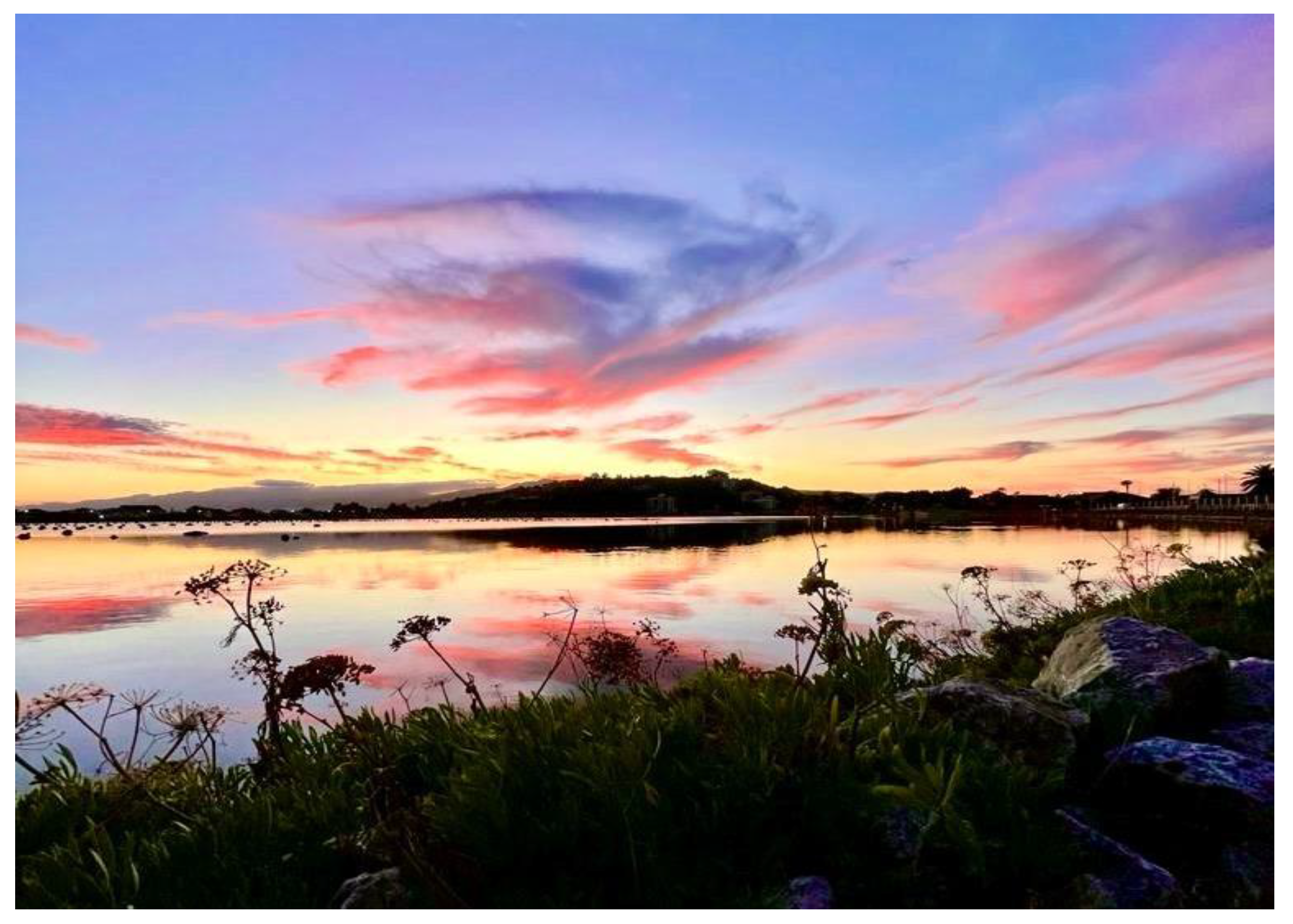
Figure 2.
(a) Geological sketch map of the north-eastern sector of Sicily, in the Peloritani Mountains (Messina). The study area (LF) in Cape Peloro is evidenced by a black rectangle. Legend: Sedimentary covers - 1) Alluvial and coastal deposits (Holocene). 2) Miocene to upper Pleistocene deposits (including the Quaternary sands and gravels of the Messina Fm). 3) Floresta calcarenites (Langhian–late Burdigalian) and Antisicilide Complex (early Miocene-late Cretaceous). 4) Stilo–Capo d’Orlando Fm (Burdigalian). Tectonic units - 5) Aspromonte Unit (a: Variscan metamorphic basement; b: Plutonic basement). 6) Mela Unit (Variscan metamorphic basement). 7) Mandanici–Piraino Unit (Variscan metamorphic basement and Mesozoic cover). (b) The black square represents the areal extension of the geological sketch map (a). The map was modified after [1].
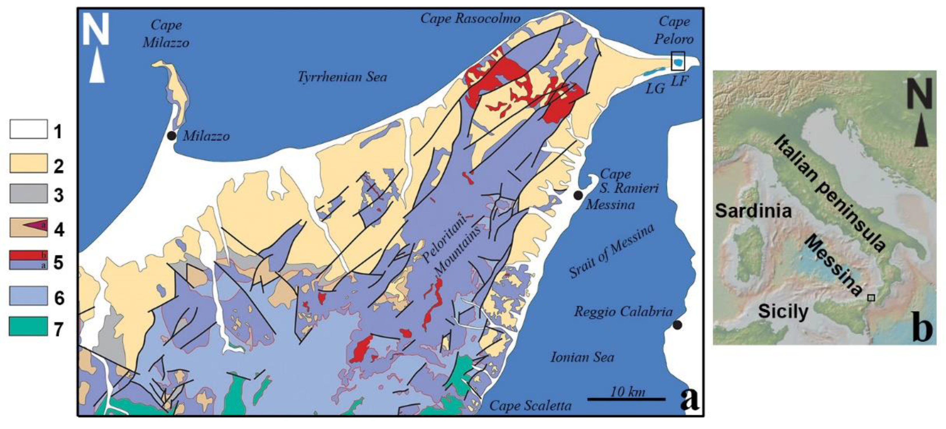
Figure 3.
Sketch structural map of the north-easternmost end of the Peloritani chain showing the main fault systems affecting the Sicilian end of the Messina Strait area (E-W trending Mortelle normal fault, NNE-SSW trending Messina normal fault system, ENE-WSW trending Scilla-Ganzirri normal fault system, NNW-SSE trending right lateral transtensive faults Faro Superiore or Curcuraci fault system). Symbols: Dashes are on the hangingwall of the normal and oblique faults; arrows indicate the right lateral strike slip component of the movement in transtensive faults. The onshore faults reported with dotted lines are uncertain. Onshore faults are as in [11,12,24,25,26] and unpublished data of the authors. The offshore faults individuated by means of seismic profiles, reported with dotted lines, are as in [17].
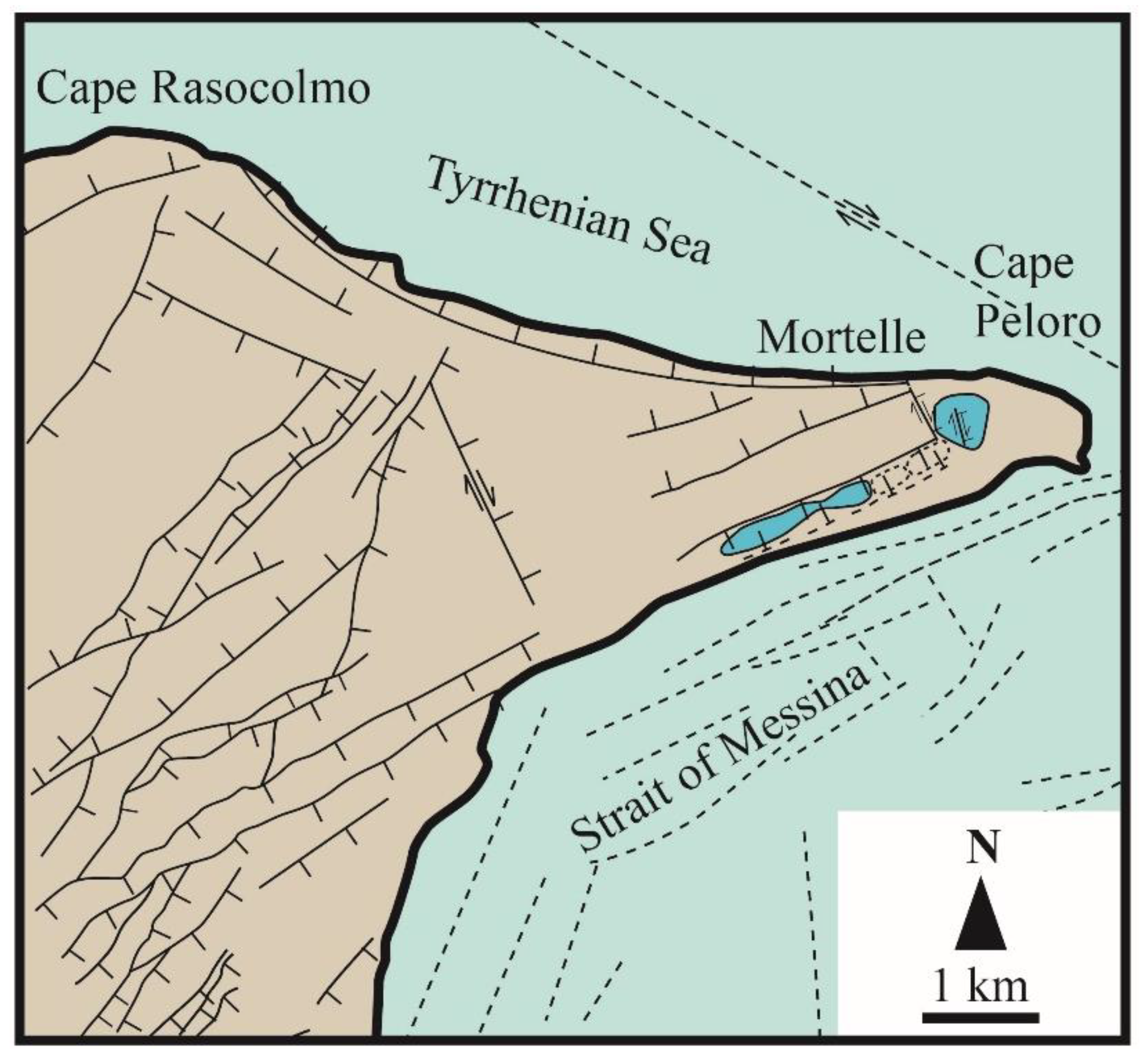
Figure 4.
Oblique aerial photo looking NNE (courtesy of Daniele Passaro) of the Cape Peloro peninsula showing the coastal lagoon with the LF to the north and the LG to the south.
Figure 4.
Oblique aerial photo looking NNE (courtesy of Daniele Passaro) of the Cape Peloro peninsula showing the coastal lagoon with the LF to the north and the LG to the south.
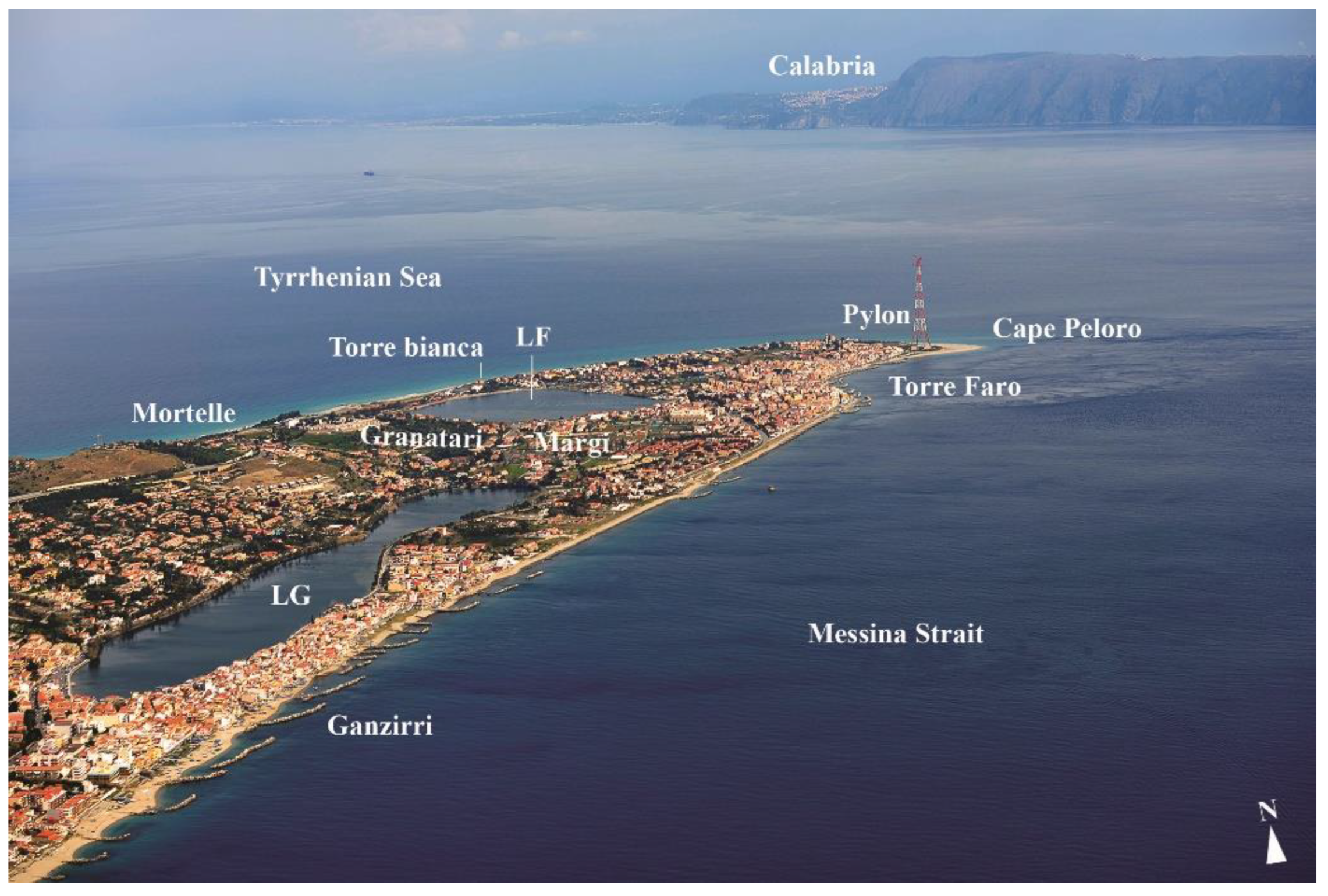
Figure 5.
Cape Peloro. (a) View from NE of the Cape Peloro peninsula and the coastal lagoon (Google Earth pro, satellite imagery). (b) Topographic map of the Cape Peloro peninsula showing the extension of the oriented natural reserve of Cape Peloro (pre-reserve in yellow color, reserve in sky blue color).
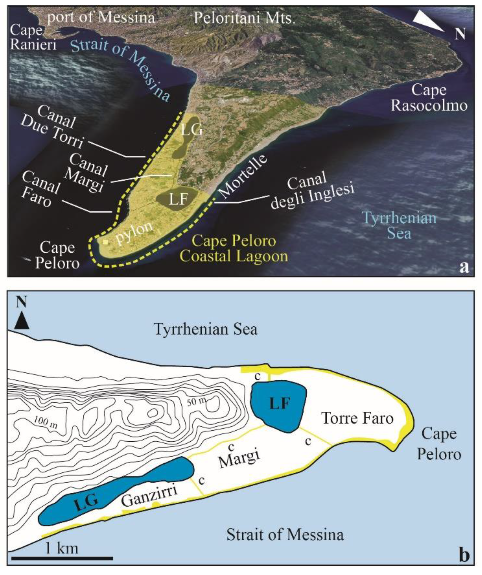
Figure 6.
Map of the LF showing the private properties’ extension and the actual area of the lake covered by farming structures. It is possible to observe the lack of correspondence among the actual area extension of farming structures (2) and the original authorized limits (3). Legend: 1) - Private properties; 2) Actual areal extension of farming structures; 3) Original authorized limits.
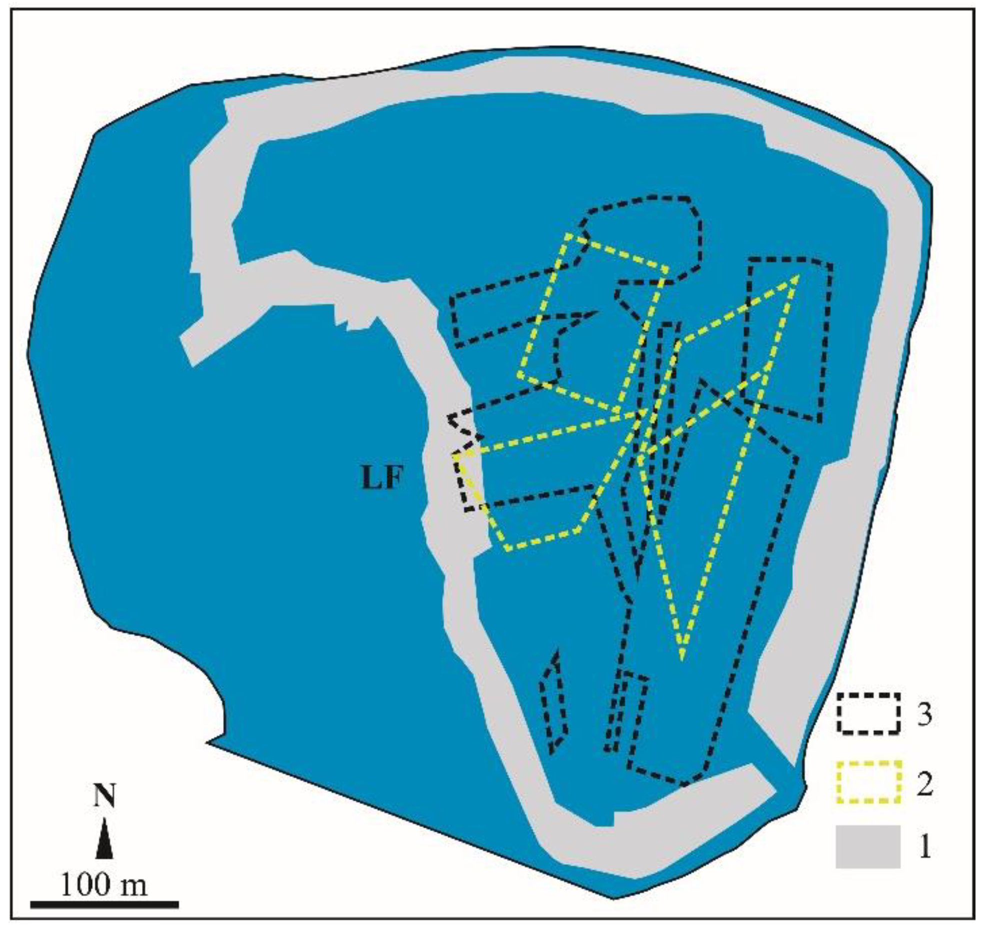
Figure 7.
Geomorphological phenomena and evolution responsible for shaping the edge of the peninsula of Cape Peloro, during the Late Pleistocene –Holocene time span [21]. (a) Deep whirl excavation because of cold currents (arrows) (Late Pleistocene). (b) Littoral sand bar shoal external to the paleo LF (Pleistocene–Holocene transition). (c) Littoral warm current circulation about 11,000–9,000 years B.P. (Holocene). Legend: 1) Middle Pleistocene substrate. 2) Palao LF. 3) Coastal deposits. 4) Marine deposits. 5) LF.
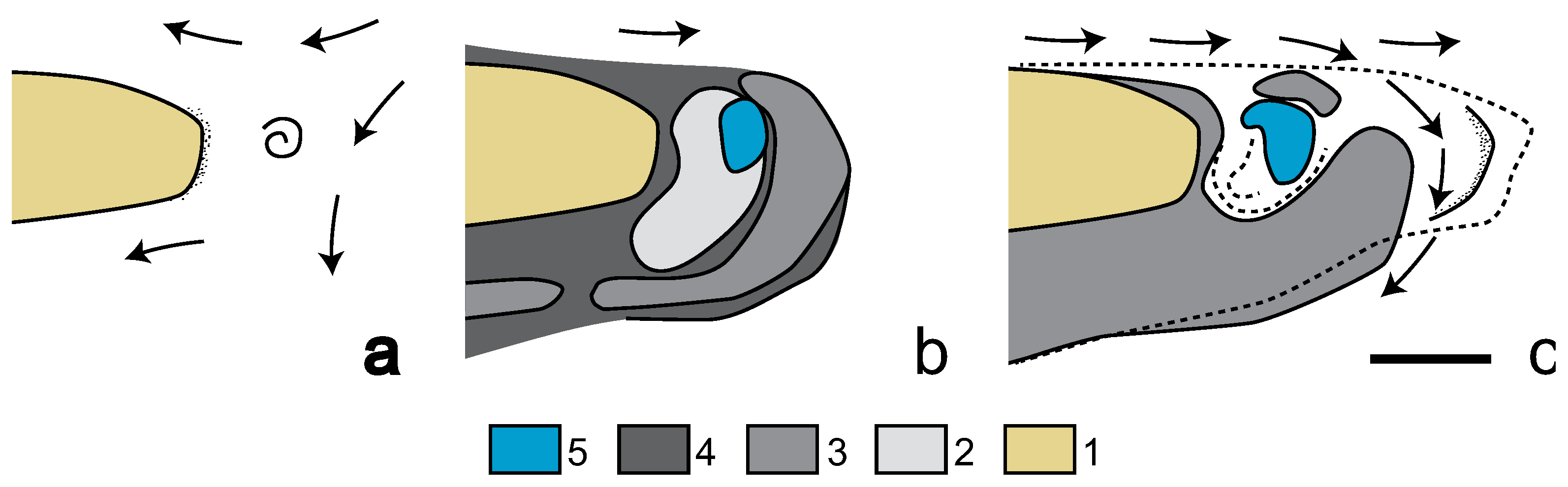
Figure 8.
Morpho–bathymetric survey of LF carried out using a single–beam ultrasound device. (a) Boat with instruments and surveying equipment. (b) 2D morpho-bathymetric colour map showing the orientation of the different measure transects. (c) Prospective satellite image of the LF (Google Earth Pro, image date: 11 July 2023). (d) 3D morpho-bathymetric colour map showing a weakly E-dipping shallow platform on the western side of the lake (plain in red colour) and a basin with a funnel-shape (blue to red colours) on the eastern side of the lake.
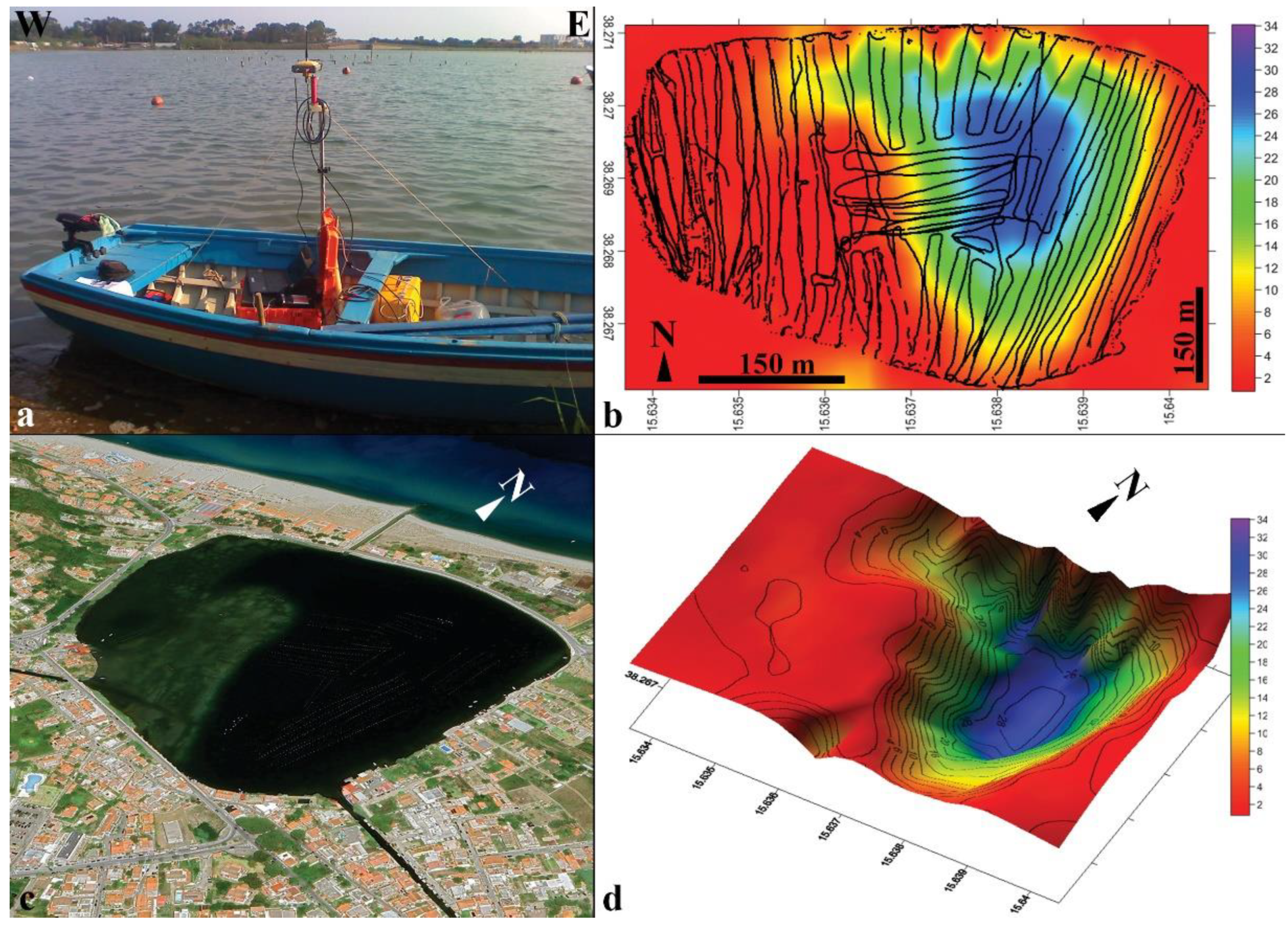
Figure 9.
Map of the samples collected along a transect E-W in the LF.
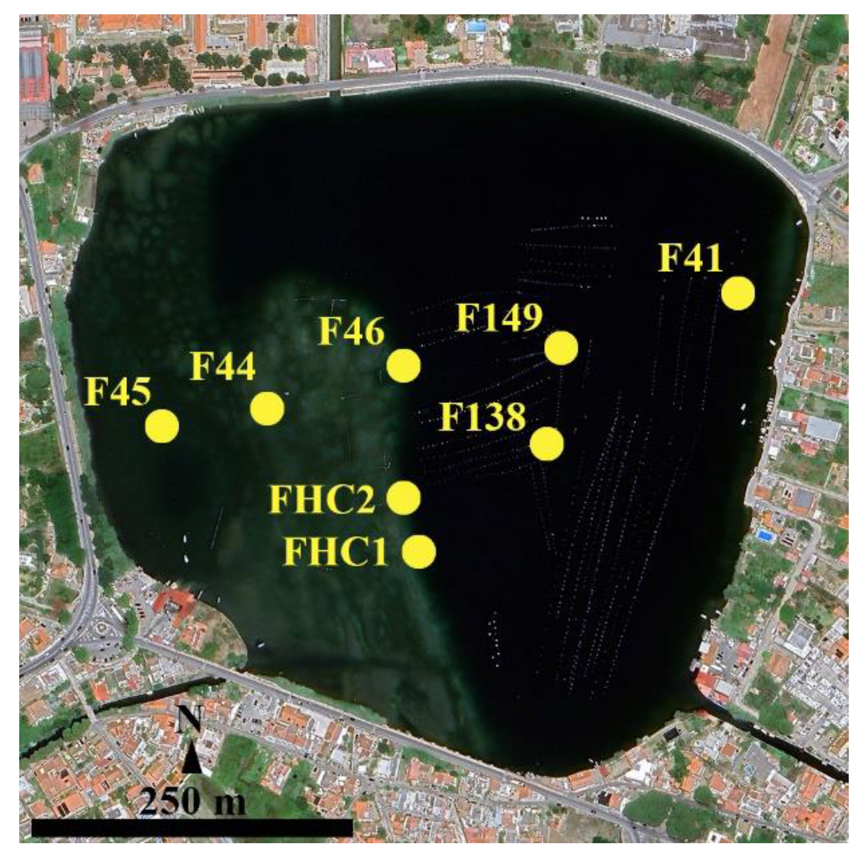
Figure 10.
Natural and anthropogenic habitats in the LF. (a-e) Shallow platform: (a) Poriferans on rhodolith beds developed on soft shell deposits, 2.5 m depth (38°16'4.27"N; 15°38'11.22"E). (b) Cymodocea nodosa beds developed on soft shell deposits and sands, 1 m depth (38°15'59.43"N; 15°38'22.96"E). (c) Natural rocky substrate rising througout the shallow lake platform, colonized by poriferans, 1 m depth (38°16'2.72"N; 15°38'13.28"E). (d) Artificial sandy mounds showing high concentration of epifaunal and infaunal organisms, 1 m depth (38°16'5.03"N; 15°38'09.84"E) (e) Highly colonized remains of an artificial substrate for clam farming, 1.5 m depth (38°16'10.94"N; 15°38'5.27"E). (f) Anoxic zone on the western slope of the deep depression, showing microbial matt, 15 m depth (38°16'4.60"N; 15°38'13.49"E).
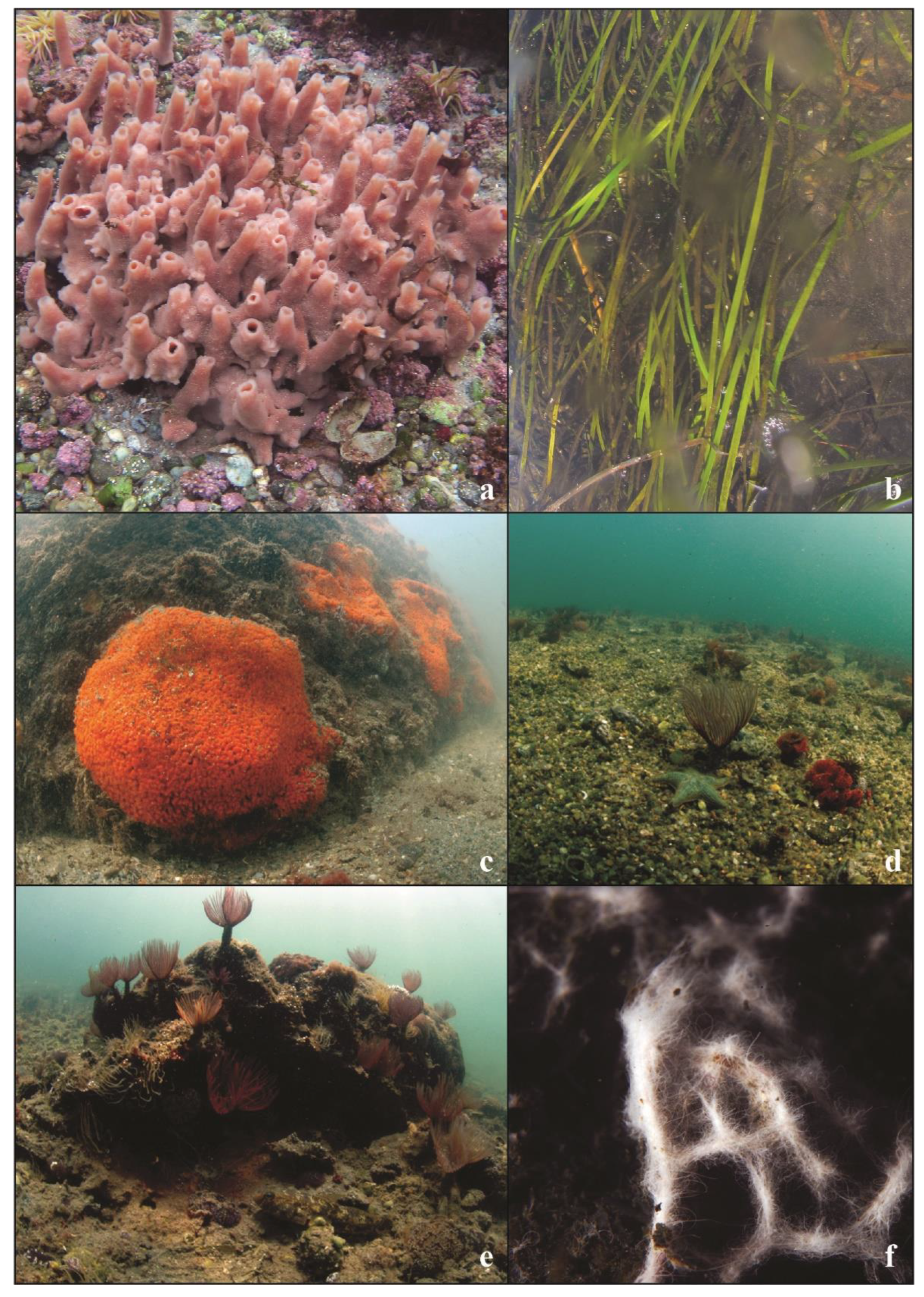
Figure 11.
PSA by laser diffraction of lacustrine sediments (samples: F45, F44, F46, F138, F149, F41). (a) Frequency curves. (b) Cumulative curves. (c) Box diagram reporting the main statistical data. Acronyms – IM: Inclusive Mean, IKs: Inclusive Kurtosis, ISk: Inclusive Skewness, ISD: Inclusive Standard Deviation.
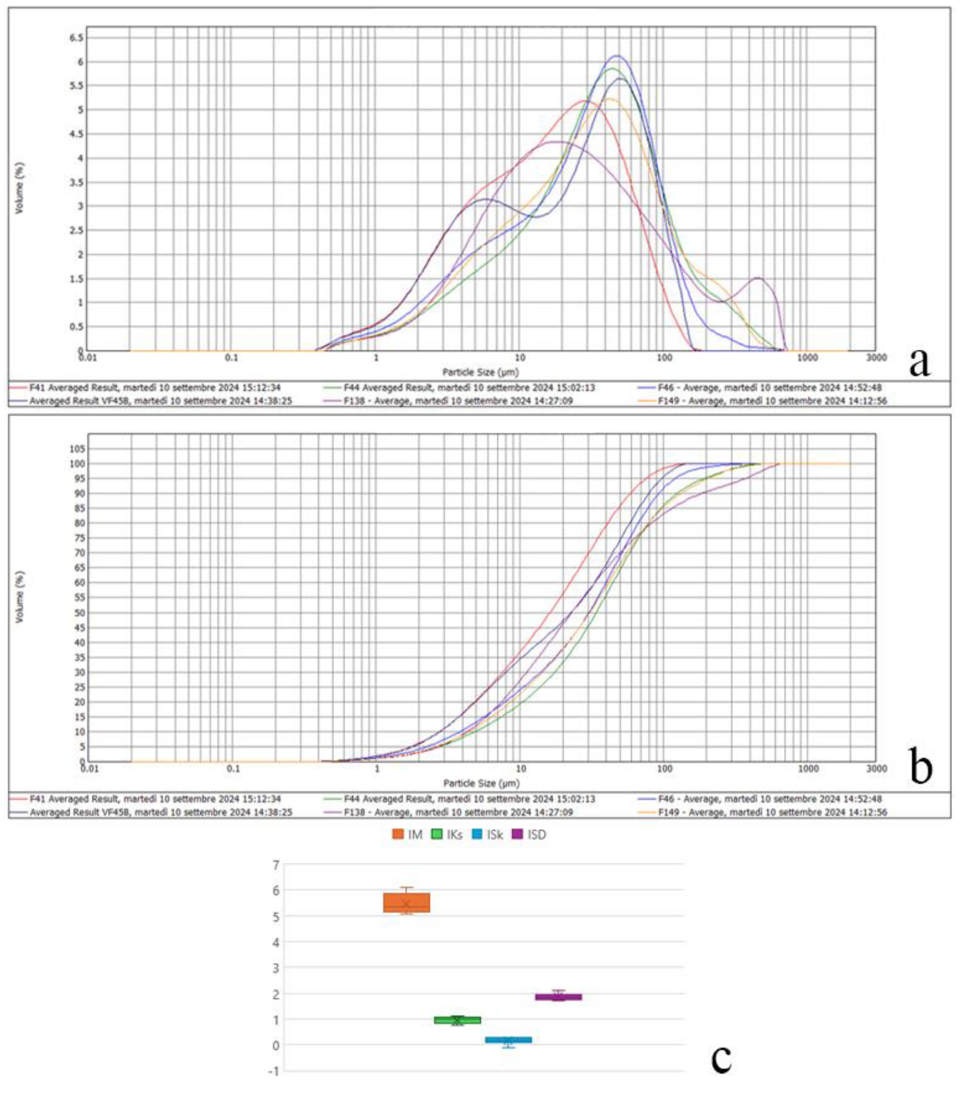
Figure 12.
(a-b). Polished sections of hard clast-supported conglomerates in sandy matrix (sample FHC01) collected along the steep cliff bounding the shallow platform.
Figure 12.
(a-b). Polished sections of hard clast-supported conglomerates in sandy matrix (sample FHC01) collected along the steep cliff bounding the shallow platform.
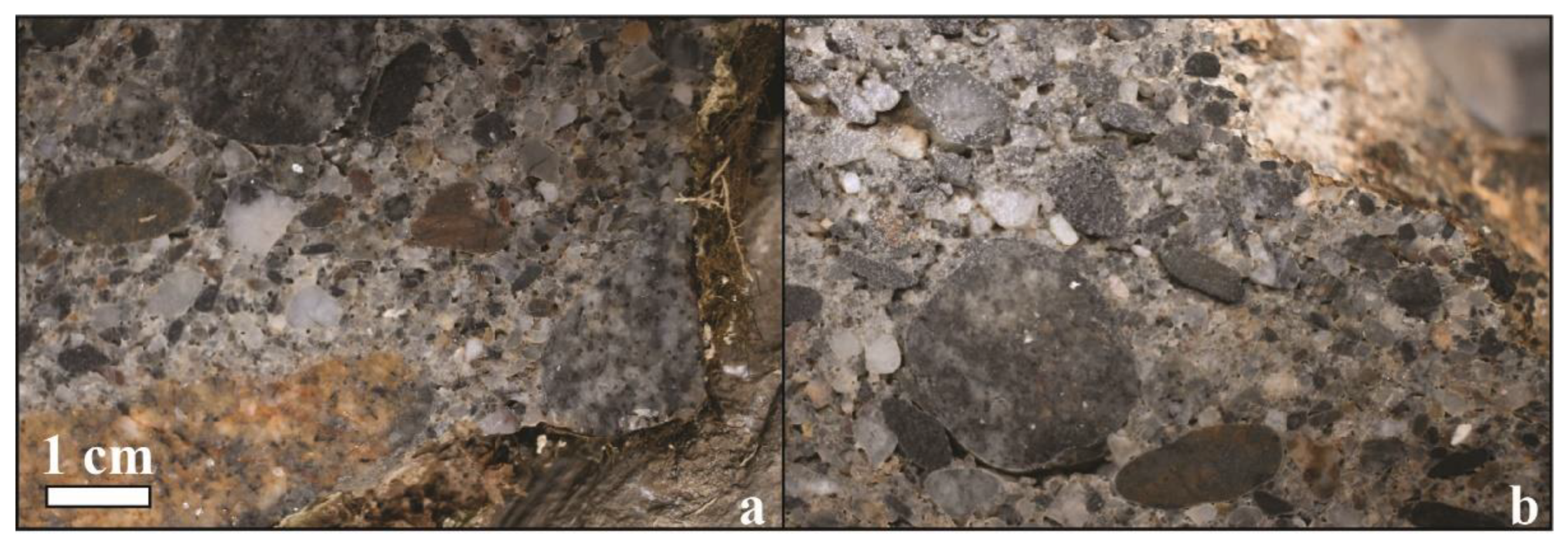
Figure 13.
Petrography of modern mineral grains from the LF soft cover, analysed in thin sections of aggregated grains in epoxy resin (sample F44). Siliciclastic grains mostly derive from erosion of metamorphic rocks and mostly appear sub–rounded. The main minerals composing the mono- and polymineral grains, in order of abundance, are: pervasively fractured quartz, plagioclase, biotite, and muscovite. Remnants of modern bioclasts (mollusks and gastropods) deriving from the mollusk farm are abundant in the sediments. (a-b) Metamorphic polymineral lithoclast, composed of quartz and plagioclase, observed under microscope, PPL (a), XPL (b). (c-d) Metamorphic polymineral lithoclast, composed of quartz and biotite, observed under microscope, PPL (c), XPL (d). (e-f) Metamorphic monomineral lithoclast composed of plagioclase preserving tabular habitus, observed under microscope, PPL (e), XPL (f). (g-h) Metamorphic polymineral lithoclast, composed of quartz and muscovite, observed under microscope, PPL (g), XPL (h). Acronyms: PPL: plane polarized light. XPL: crossed polarized light. Scale bar is the same in all the images.
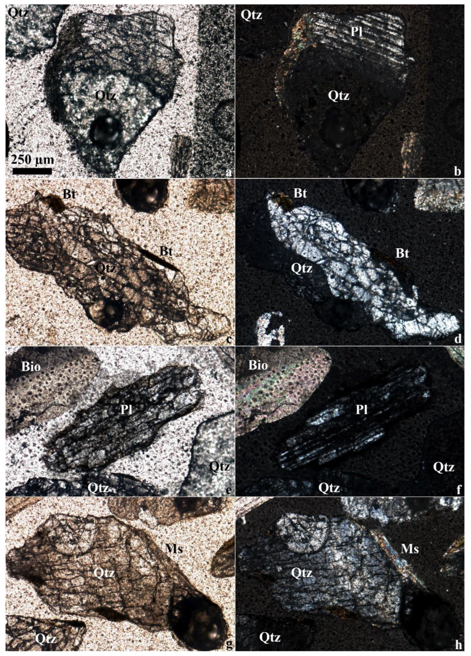
Figure 14.
Main macroscopic faults present on the study area. (a) Lake Faro transtensive Fault (LFF) observed on an oblique aerial photo of the LF looking ENE-wards. Other faults are also present (Mortelle normal Fault (MF), Ganzirri normal Fault (GF), Faro transtensive Fault (FF). (b) LFF observed on an oblique aerial photograph of the LF looking NW–wards. (c) Subaqueous photograph of the LFF scarp. The fault bounds the shallow platform (on the left) and appears overlain by soft cover.
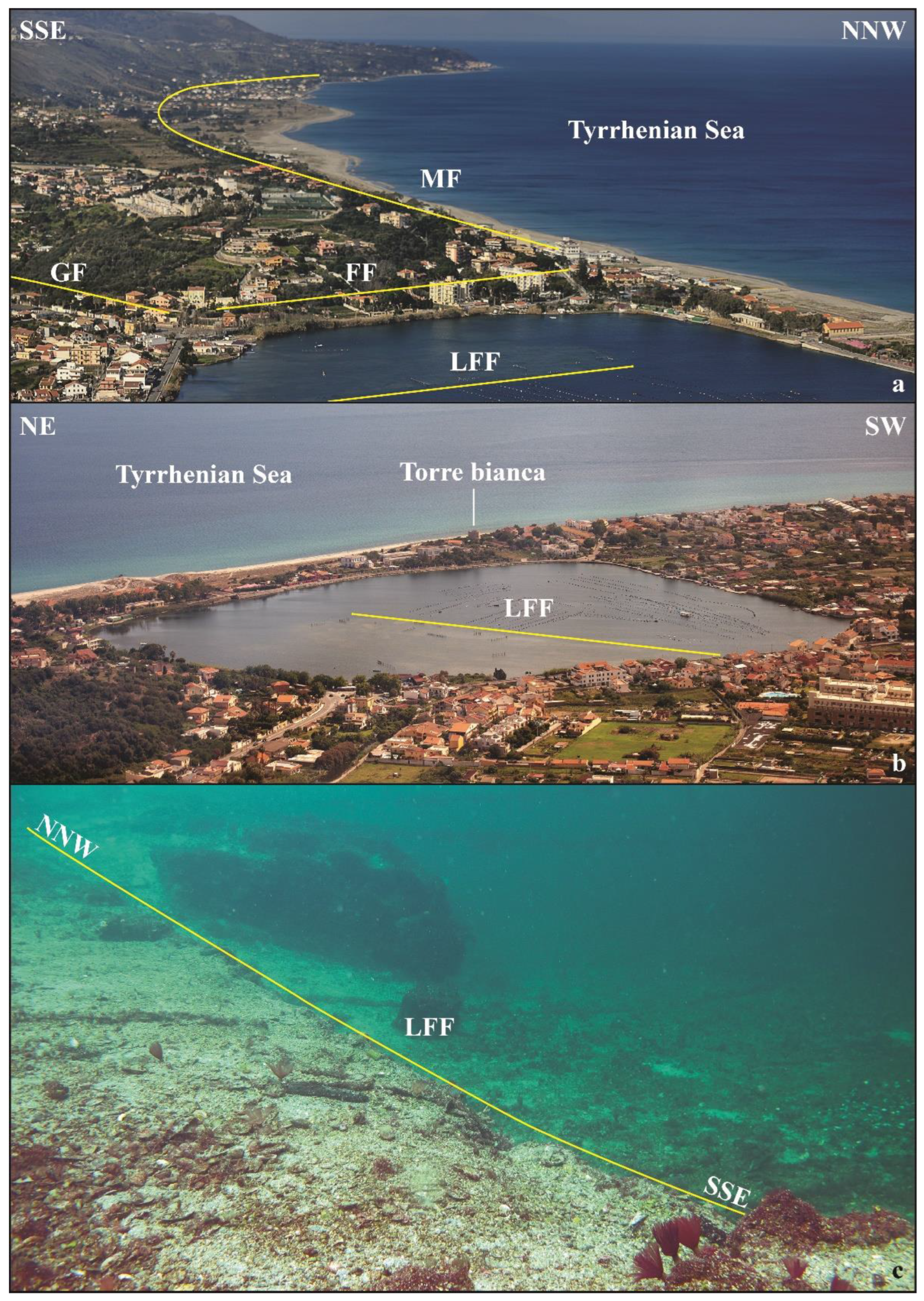
Figure 15.
Photographs (letter) and line drawings (letter ‘) of the mesoscale faults affecting the Quaternary deposits. (a-a’, b-b’, c-c’, d-d’, e-e’): ENE-WSE trending normal faults of the Scilla Ganzirri fault system (faults reported in orange color). (f-f’, g-g’): NNE-SSE dextral transtensive faults of the Faro Superiore fault system (faults reported in blue color). Coordinates of the faults: (a-a’): 38°24’0.47”N; 15°55’49.16”E. (b-b’): 38°24’0.568”N; 15°55’47.25”E. (c-c’): 38°26’4.835”N; 15°60’92.66”E. (d-d’): 38°24’0.568”N; 15°55’47.25”E. (e-e’): 38°24’0.802”N; 15°55’46.19”E. (f-f’): 38°26’4.86”N; 15°61’08.25”E. (g-g’): 38°26’4.86”N; 15°61’08.25”E.
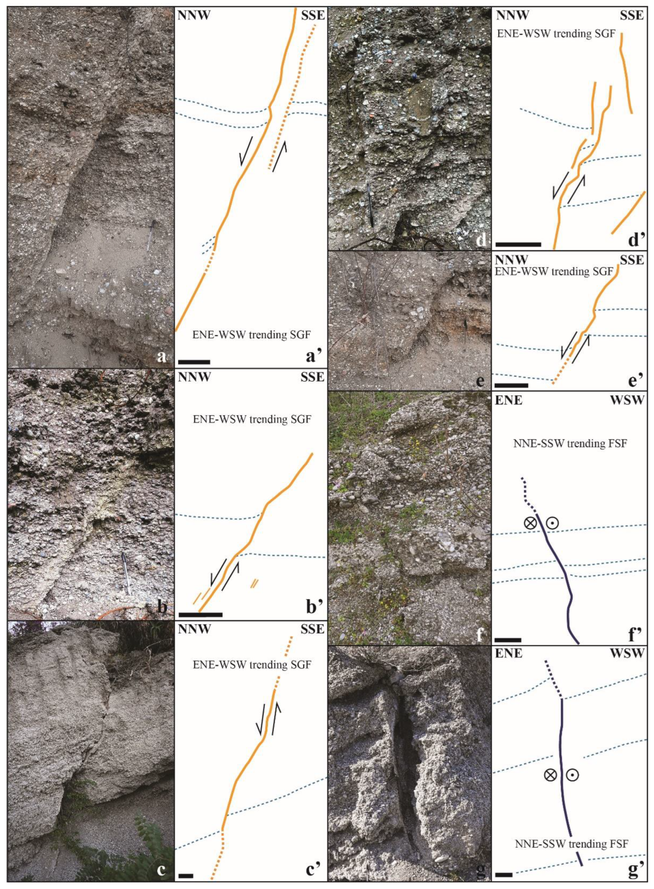
Figure 16.
Interpretative sketch maps showing the main macroscale faults affecting the Cape Peloro peninsula in the late Pleistocene-Holocene time span. Faults are reported on a topographic surface showing different elevations on the sea level (according to [29] modified). (a) Present day topographical surface. (b) Holocene topographical surface with Δh variation of sea-level of +1.00. (c) Holocene topographical surface with Δh variations of sea-level of +2.00 m. Reference point: Torre bianca (black circle). Acronyms: LFF - Lake Faro Fault; FF – Faro Fault; MF – Mortelle Fault; GF – Ganzirri Fault; GAF – Ganzirri Antithetic Fault.
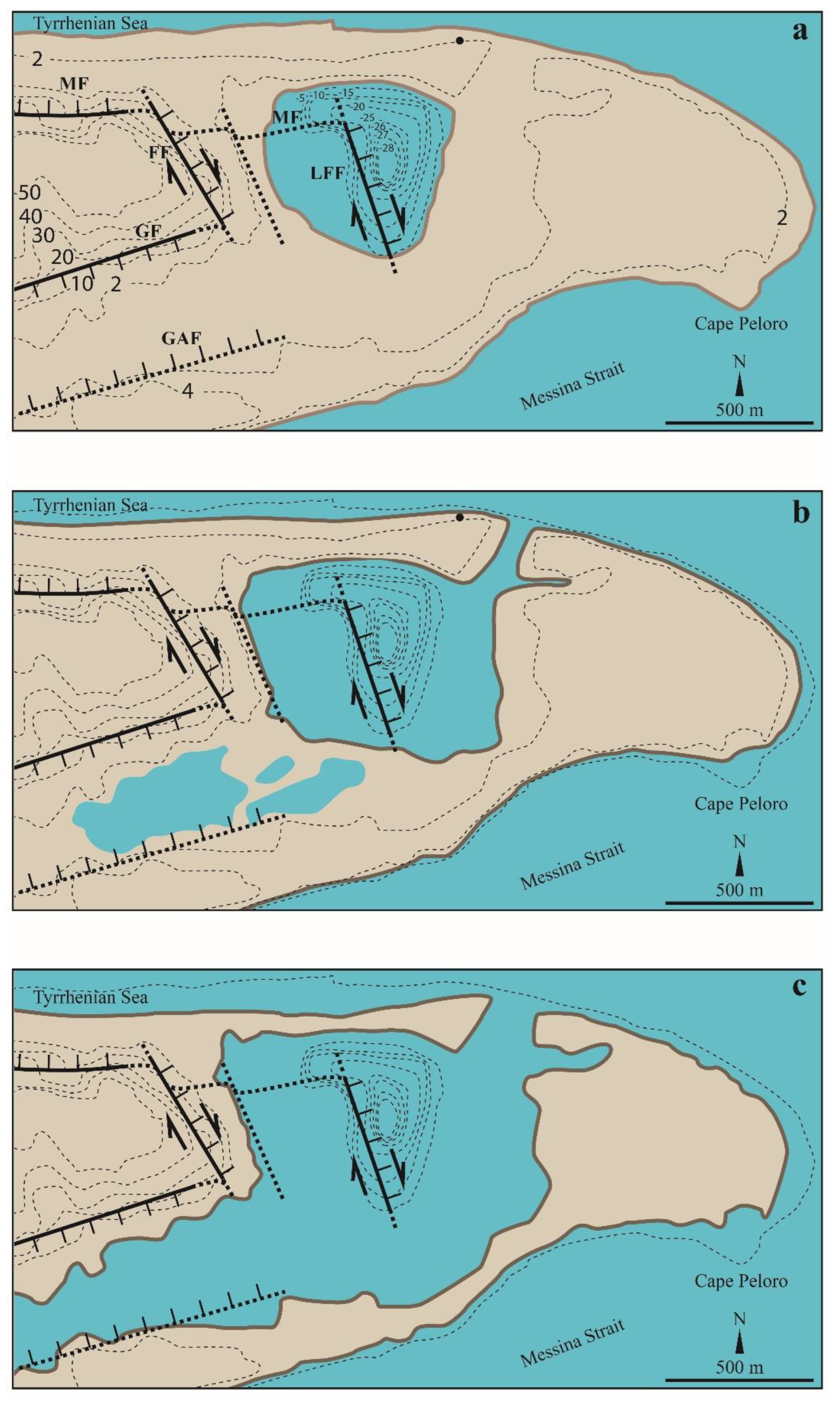

Table 1.
Geographic coordinates and depths of the samples collected along a transect E-W in the LF, from West to East.
Table 1.
Geographic coordinates and depths of the samples collected along a transect E-W in the LF, from West to East.
| ID Sample | Deposits | Latitude | Longitude | Depth (-m) |
|---|---|---|---|---|
| F45 | Soft cover | 38° 16' 06.840" N | 15° 38' 04.368" E | 2.50 |
| F44 | Soft cover | 38° 16' 07.092" N | 15° 38' 07.938" E | 2.50 |
| F46 | Soft cover | 38° 16' 08.280" N | 15° 38' 12.408" E | 8.00 |
| F138 | Soft cover | 38° 16' 06.258" N | 15° 38' 17.028" E | 27.00 |
| F149 | Soft cover | 38° 16' 08.712" N | 15° 38' 17.640" E | 28.00 |
| F41 | Soft cover | 38° 16' 10.290" N | 15° 38' 23.540" E | 7.00 |
| FHC1 | Hard conglomerate | 38° 16' 03.080" N | 15° 38' 12.094" E | 4.00 |
| FHC2 | Hard conglomerate | 38° 16' 04.710" N | 15° 38' 12.054" E | 4.00 |
Table 2.
Classification of the soft cover samples, as it was (bioclasts and sediments), on the base of mechanical sieving.
Table 2.
Classification of the soft cover samples, as it was (bioclasts and sediments), on the base of mechanical sieving.
| ID Sample | Gravel (%) | Sand (%) | Mud (%) | Classification |
|---|---|---|---|---|
| F45 | 13.22 | 81.72 | 0.060 | “Shell-rich gravelly sand" |
| F44 | 51.66 | 47.69 | 0.640 | Sandy gravel |
| F46 | 65.3o | 29.64 | 5.060 | “Shell-rich gravel with sand” |
| F138 | 29.00 | 19.20 | 51.90 | Mud with sandy gravel |
| F149 | 27.60 | 19.30 | 53.10 | Mud with sandy gravel |
| F41 | 46.05 | 53.50 | 0.430 | Gravelly sand |
Table 3.
Statistical data on the LF sediments obtained by means of PSA laser diffraction. Acronyms – Percentiles d(0.1), d(0.5), d(0.9): size below which 10%, 50% or 90% of all particles. IM: Inclusive Mean, IKs: Inclusive Kurtosis, ISk: Inclusive Skewness, ISD: Inclusive Standard Deviation.
Table 3.
Statistical data on the LF sediments obtained by means of PSA laser diffraction. Acronyms – Percentiles d(0.1), d(0.5), d(0.9): size below which 10%, 50% or 90% of all particles. IM: Inclusive Mean, IKs: Inclusive Kurtosis, ISk: Inclusive Skewness, ISD: Inclusive Standard Deviation.
| ID Sample | d(0.1) | d(0.5) | d(0.9) | Mode | IM | IKs | ISk | ISD |
|---|---|---|---|---|---|---|---|---|
| µm | phi | |||||||
| 45 | 2.84 | 23.09 | 80.02 | 53.09 | 5.77 | 0.78 | 0.26 | 1.88 |
| 44 | 5.01 | 34.50 | 126.36 | 44.98 | 5.07 | 1.11 | 0.18 | 1.80 |
| 46 | 3.93 | 30.70 | 94.04 | 48.40 | 5.36 | 0.96 | 0.29 | 1.77 |
| 138 | 6.47 | 40.44 | 184.11 | 47.35 | 4.73 | 1.02 | 0.10 | 1.86 |
| 149 | 4.53 | 30.99 | 134.74 | 43.29 | 5.20 | 1.02 | 0.13 | 1.89 |
| 41 | 2.82 | 16.48 | 59.52 | 29.34 | 6.09 | 0.88 | 0.16 | 1.71 |
Disclaimer/Publisher’s Note: The statements, opinions and data contained in all publications are solely those of the individual author(s) and contributor(s) and not of MDPI and/or the editor(s). MDPI and/or the editor(s) disclaim responsibility for any injury to people or property resulting from any ideas, methods, instructions or products referred to in the content. |
© 2024 by the authors. Licensee MDPI, Basel, Switzerland. This article is an open access article distributed under the terms and conditions of the Creative Commons Attribution (CC BY) license (http://creativecommons.org/licenses/by/4.0/).
Copyright: This open access article is published under a Creative Commons CC BY 4.0 license, which permit the free download, distribution, and reuse, provided that the author and preprint are cited in any reuse.


