Submitted:
07 October 2024
Posted:
08 October 2024
You are already at the latest version
Abstract
The study investigates methods to enhance the reliability of NO2 monitoring using low-cost electrochemical sensors to measure gaseous pollutants in air by addressing the impacts of temperature and relative humidity. The temperature within a plastic container was controlled using an internal mica heater, an external hot air blower or cooling packs, while relative humidity was adjusted using glycerin solutions. Findings indicated that the Auxiliary Electrode (AE) signal is susceptible to temperature and moderately affected by relative humidity. In contrast, the Working Electrode (WE) signal is less affected by temperature and relative humidity; however, adjustments are still required to determine gas concentrations accurately. Tests involving on/off cycles showed that the AE signal experiences exponential decay before stabilizing, requiring the exclusion of initial readings during monitoring activities. Additionally, calibration experiments in zero air allowed the determination of the compensation factor nT across different temperatures and humidity levels. These results highlight the importance of compensating for temperature and humidity effects to improve the accuracy and reliability of NO2 measurements using low-cost electrochemical sensors. This refinement makes the calibration applicable across a broader range of environmental conditions. However, the experiments also show a lack of repeatability of the zero calibration.
Keywords:
Calibration
; Repeatability
; NO2 monitoring
; Low-cost sensors
; Temperature compensation
; Humidity effects
1. Introduction
According to the Environmental Protection Agency (EPA)’s 2017 National Emission Inventory, 52% of nitrogen dioxide (NO₂) emissions originate from mobile sources such as cars, trucks, and planes, while 32% originate from stationary sources such as power plants or cement kilns [1] The transport sector produces NO₂ primarily through combustion engines, where nitrogen gas (N2) in the air is converted into oxides when fuel burns in excess of oxygen at temperatures exceeding 1300°C [2,3]. Unfortunately, NO₂ is a significant air pollutant that substantially impacts human health. The World Health Organization (WHO) has highlighted numerous health risks and fatalities associated with NO₂ exposure [4]. Research indicates that exposure to NO₂ can lead to premature death [5] from respiratory, cardiovascular [6,7,8,9,10] and circulatory illnesses, as well as the development of asthma [11] and bronchitis [12,13,14,15]. NO₂ is particularly concerning due to its role in increasing the risk of childhood asthma [16,17,18,19], a major global health issue.
Monitoring NO₂ typically involves continuous measurement techniques using the chemiluminescence method described in ISO standard 7996:1985 [20]. This method is considered the reference method for environmental regulatory monitoring. However, it is expensive to purchase, operate, and maintain. An alternative is the use of active samplers, which pump air through an azo-dye-forming reagent to produce a pink color as detailed in ISO 6768:1998 [21]. Although this method is highly sensitive, it is also labor-intensive, requires skilled personnel, uses potentially harmful chemicals, and is unsuitable for sampling periods longer than 1-2 hours [22,23,24]. Passive samplers, where the pollutant diffuses toward the absorbent, offer an alternative by assessing ambient NO₂ levels without needing electric power at the deployment site [22,23,25,26,27,28,29]. However, these samplers provide only an average concentration over a week or longer, failing to capture daily variations in NO₂ concentrations and making them unsuitable for identifying short-term pollution events. Additionally, the collected samples must be analyzed in a laboratory, which is time-consuming and costly [30].
Low-cost sensors can provide highly time-resolved data, enabling better identification of pollution variations and real-time data [12,31,32,33,34,35,36] without additional laboratory work [12]. Their affordability, compact size, and quick response times make them valuable for low-income countries [37]. However, the reliability of these devices is often questioned, especially when benchmarked against the gold standard. Issues such as cross-sensitivities, calibration drift over time, short life expectancies, low sensitivities, and variability due to environmental conditions challenge their accuracy [30,31,34,38,39,40,41,42,43,44]. Additionally, the performance of these sensors in tropical conditions, like those in Cuba where temperatures can exceed 30°C and relative humidity is often above 90%, remains uncertain.
This study examines the potential for improving the calibration of the Alphasense NO2-A43F sensor [45]. Although the manufacturer provides a calibration document, its validity under conditions different from the original calibration environment remains uncertain. Various calibration methods have been proposed to enhance the data quality of low cost sensors, often involving complex laboratory setups, high-end reference instruments, or advanced mathematical techniques such as machine learning [31,34,36,46,47,48,49,50,51,52,53,54]. This study aims to improve the calibration method using low-cost setups and straightforward methods that can be implemented with commonly used software applications such as Microsoft Excel. This approach makes it feasible for low-income countries to conduct independent measurement campaigns with reasonable reliability. Specifically, the study will focus on the impact of temperature and relative humidity on the sensor’s calibration.
2. Background
Electrochemical four-electrode gas sensors, such as those from Alphasense, are widely used for air quality monitoring due to their good sensitivity and selectivity. In combination with the Alphasense Analog Front-End (AFE) sensor board, these sensors register voltages from the working electrode (WE) and the auxiliary electrode (AE). The WE electrode generates a signal proportional to the concentration of the target analyte, while the AE electrode, which is buried within the sensor, accounts for temperature and humidity changes. Despite the manufacturer’s calibration information, accurately calculating pollutant concentrations remains challenging. More accurate calibration requires a better understanding of the compensation factor nT, defined as the ratio WE/AE for zero air at the measurement’s temperature and relative humidity. The manufacturer provides different nT values and calculation formulas for determining the concentration of the target analyte across several documents [55,56,57], leading to confusion. Previous work described the basic formulas used to convert the WE signal generated by the target analyte into a concentration, considering nT as a constant [58]. The measured WE signal comprises a background component WEbackground not generated by the target analyte but that is affected by temperature and relative humidity, and a portion that is proportional to the concentration of the target analyte, WEgas. The variables used in eq. 1 and 2 are defined in Table 1.
3. Materials and Methods
3.1. Design of the Low-Cost Data Logger
A low-cost, custom-built data logger uses the Arduino Mega 2560 microcontroller as its core component. To enhance its versatility and allow users to tailor it to their specific needs, a compact, custom-designed expansion shield has been developed [59,60,61]Haga clic o pulse aquí para escribir texto. No changes have been made to the hardware during this work. The expansion shield enables the connection of sensors to the data logger and converts sensor signals into a format that the microcontroller can interpret. In this setup, NO2 has been measured with the NO2-A43F sensor (Alphasense, United Kingdom). The gas sensor is integrated into an Alphasense AFE board (model 810-0023-00), which is connected to the expansion shield via a flat cable and appropriate connectors. Temperature and relative humidity are measured using two sensors: the SCD30 (Sensirion, Switzerland) and the AM2315C (Asair, China).
3.2. Sensor Calibration Experiments
Calibration experiments were performed in a sealable plastic box equipped with various components to allow for the introduction and control of calibration gases. A syringe filled with calibration gas can be connected to the box through a valve mounted on its lid (3-Way Blue Sterile Stopcock for Intravenous Drips). Inside the box, a fan and a mica heater work together to ensure efficient mixing and precise temperature control. The wires powering these components were routed through a pre-drilled hole, which was securely resealed with hot glue to maintain an airtight seal. For certain experiments, the box was insulated with bubble wrap. Additionally, the side of the box includes two valves that can be coupled to a closed loop, allowing air to be pumped through a wash bottle to effectively remove small concentrations of NO2 from the ambient air enclosed in the box. A similar setup was used in previous experiments [37,58,60].
The calibration gas is generated using the stoichiometric reactions R1 and R2 [65,66,67] with a set-up described earlier [37,58]. One syringe of 6 mL contains 0.4 mL of 0.18 mol/L FeSO4.7H2O dissolved in 20 vol% HCl and the second syringe of 6 mL contains 0.2 mL of 1.31 mol/L NaNO2 solution. The reagents are brought together to generate 1.9 mL of NO gas in a third syringe (reaction R1). All syringes are connected using 3-way valves. To obtain NO₂ gas, it is necessary to aspirate 0.2 mL of air into the third syringe (reaction R2). The amount of NO2 inside the syringe is calculated using the ideal gas law as described earlier [58]Haga clic o pulse aquí para escribir texto..
The sealable calibration box, along with the setup designed to generate calibration gas in a syringe, has been utilized to conduct several calibration experiments. All experiments described in the list below have been performed within a period of 2 months.
- Stability of the sensor signal during repeated on/off cycles of the system: To evaluate the stability and repeatability of the sensor signal under cyclic operational conditions, measurements were conducted in a closed box, where the system was repeatedly switched on and off. Two tests were performed, each with a 10-minute turn-on period. In the first test, the switch-off intervals were fixed at 5 minutes, whereas in the second test, the switch-off period was gradually increased from 1 to 5 minutes. Each cycle was repeated five times. For every cycle, the average and standard deviation of the signal during the final minute were calculated and compared across cycles.
- Sensor shocks caused by temperature: The sensor was subjected to temperature shocks, with sudden temperature increases in the calibration box achieved through two methods: 1) an internal heating element (Mica Heating Pad, 80 W, 230 V AC, RS PRO) controlled externally via a digital regulator (Digital LED Thermostat Temperature Controller with Sensor Probe, MH1210A Mini, 12 VDC, Amazon), and 2) an external hair dryer directed towards the lid of the calibration box.
- Sensor shocks caused by concentrations: During the experiment, excess NO₂ gas was injected into the calibration box through a valve mounted on the lid of the calibration box.
- Evaluation of the impact of T on sensor signal: The impact of temperature on the NO2 sensor calibration has been assessed by analyzing the sensors in zero air. Zero air was generated by pumping the air from the sealed box through a gas wash bottle containing a saturated Ca(OH)₂ solution. This setup is followed by a second bottle designed to capture any small droplets and a tube filled with silica gel to maintain a constant relative humidity within the box. To lower the internal temperature below ambient conditions, cooling packs were applied to the exterior walls of the calibration box. The box and the cooling packs are insulated with bubble wrap. After the temperature stabilizes at approximately 14°C, the cooling packs are removed, allowing the system to gradually return to ambient temperature. Subsequently, a hair dryer is used to externally heat the calibration box lid until the temperature reaches 42°C. The system was then left to cool freely back to ambient temperature. Throughout the experiment, there was no control over relative humidity (RH) within the box to keep it constant. As a result, RH naturally increased during cooling and decreased during heating to some extent. This setup enabled the determination of the factor nT as a function of temperature.
- Evaluation of the impact of RH on sensor signal: The impact of relative humidity on the NO2 sensor signals is analyzed by measuring WE and AE signals over time in clean ambient air at room conditions (approximately 29°C and 30% RH). The experiment was conducted in laboratory ambient air conditions, as these conditions yield, WE_NO2 and AE_NO2 values that are comparable to those obtained when zero air is generated. To adjust the RH, the lid of the box was opened and a Petri dish containing 200 mL of a glycerine solution was introduced into the calibration box. The large-sized Petri dish with a diameter of 15 cm provides a large contact area between the solution and the air enclosed in the container. A fan is used to homogenize the air inside the box, ensuring an even distribution of humidity. During the experiment, the RH inside the closed box gradually adjusts towards the new equilibrium. It is observed that the introduction of the Petri dish caused a sudden temperature drop of about 2°C in all experiments. The setup enabled the determination of the factor nT as a function of relative humidity with minor temperature changes.
- Sensor response to the target analyte: The effect of the NO2 concentration on the gas sensor has been evaluated by introducing known amounts of NO2 gas inside the closed plastic box containing the NO2 gas sensor. Before the calibration test, the air is first purified using the same method described in the previous experiment. The cleaned air is used to determine WE and AE in zero air. Subsequently, controlled amounts of NO2 are generated as previously stated. The pure NO2 gas, held within a syringe, is first diluted by introducing the gas into a second plastic box for dilution (2 mL in a box of 6.1655 L). After approximately 20 minutes, a sequence of gas volumes (0.5, 1, 1.5, 2, and 2.5 mL) is taken from the dilution box and introduced into the calibration box. Each injection results in a calibration point where sensor signal WEgas and corresponding pollutant concentration is known. The sensor’s sensitivity is determined by performing a linear regression on these data points. The refined quantification method was assessed by processing conditions with known NO2 concentrations at different temperatures.
4. Discussion
4.1. Repeated On/Off Cycles of the System
Figure 1 illustrates the behavior of the AE and WE signal of the NO2 sensor over time during on/off cycles. The most notable observation is the substantial difference between the two signals: (1) the WE signal remains stable over time, and (2) the AE signal is initially high when the system is switched on, but then drops exponentially until it stabilizes. This exponential decay pattern is observed in all cycles and takes about 4 minutes. This indicates that after switching on the system some time is needed to reach stabilization and this period should be disregarded from the monitoring campaign. The initial AE signal observed immediately after switching on the system increases as the off-period lengthens. This result is in line with those reported by other authors, who have found that, in addition to temperature, relative humidity and other compounds, the response of the sensor is influenced by its specific characteristics, such as heating time, electrical signal gain and the manufacturer’s initial calibration [36,50].
The repeatability of measurements under identical conditions is crucial for sensor reliability. Therefore, the values of the WE and AE after stabilization have been determined and compared with each other. Table 2 gives for both experiments an overview of the average values and their standard deviations of the last minute of each cycle. The values in all columns in Table 2 appear to slightly drop over time, suggesting that stabilization requires more time. According to the t-test, the difference between the minimum and maximum values in each column is significant. Moreover, the variation of the signals within the stable parts of the cycles is smaller than the differences between the cycles. The experimental values for WE closely match the certified value (see section 4.7). However, the AE shows a significant deviation from the certified value, which may be due to the higher temperature at which the experiment is conducted. The experiments indicate adequate repeatability over short time periods, but this repeatability deteriorates as time progresses.
4.2. Impact of Temperature Shocks on the Sensor
Figure 2 illustrates the variation in the WE and AE signals from both the working and auxiliary electrodes as temperature increases. Figure 2a shows that when the mica heater is activated, the AE signal rapidly increases, reaching saturation at approximately 5000 mV, while the WE signal sharply decreases. Although the fan homogenizes the air inside the calibration box, it is possible that the air temperature at the top of the sensor is not identical to the air temperature measured by the temperature sensors about 10 cm away from the gas sensor. Additionally, the emission of thermal radiation by the mica heater and its impact on the sensor is not affected by the fan. The experiment shows that the change in the AE signal is not only determined by the temperature itself but also by the heating process itself. This can be seen by the difference in the AE signal behavior when using the internal heater (saturation of the AE signal in Figure 2a) and the external heater (small increase in signal shown in Figure 2b with a maximum value of 424 mV). In both cases the temperature is measured by the same sensor inside the box raised up to around 40°C.
In Figure 3a, the controller of the mica heater was used to increase the temperature inside the box in steps of 5°C. The experiment was started at a room temperature of around 25 °C, then the external heater was set to 30 °C for 2 hours and then to 35 °C for a further 2 hours. During this experiment, the AE signal did not reach saturation but showed unrealistically high values, which were never observed during monitoring campaigns in Belgium’s summer or in Cuba’s tropical climate. The WE signal showed small increases during the sudden temperature rise. It did not exhibit the drop as observed in Figure 2a. External heating of the air inside the calibration box appeared to be a better method with higher control. However, in Figure 3b, a sudden but slight drop in the AE signal can be observed for a brief period when the temperature started to rise. This suggests that temperature changes must be introduced carefully. A significant temperature shock causes the AE signal to rapidly increase and reach saturation, while a more gradual shock results in a sudden drop in the AE signal. Also, for WE an opposite behavior is observed. Any temperature shock results in a strong but erroneous sensor response.
4.3. Concentration Shocks
In Figure 4, 2.0 mL of pure NO2 gas are injected into the calibration box using a syringe. The WE-signal rises sharply and reaches saturation. The sensor board is powered with 5000 mV and it cannot generate a signal larger than the input voltage. In addition, the behavior of the AE-signal is supposed to be independent of the concentration of the target analyte but during these circumstances, the signal dropped to 0 mV. After saturation is reached, the calibration box is opened to reduce the NO2 concentration and then closed to remove the remaining NO2 by bubbling the gas through a saturated Ca(OH)2 solution. In this way, the WE gradually decreased over time. After stabilization, The WE and AE-values before and after the concentration shock were significantly different (WE: 289 vs. 304 mV; AE: 537 vs. 516 mV). This suggests that concentration shocks during a monitoring campaign can affect the calibration. Also, the constant nT is affected by the concentration shock (0.5382 vs. 0.5891).
4.4. Impact of Temperature on nT
The time series collected during the experiment in Figure 5 indicates that the AE signal is significantly influenced by temperature. For the WE signal, the impact of temperature is weaker but still significant enough to necessitate compensation for accurate gas concentration calculations. The experimentally determined values for WE0 and AE0 at a temperature of 23 ± 2°C are 275.4 mV (Alphasense value: 281 mV) and 249.8 mV (Alphasense value: 290 mV) respectively. The WE-value appears to be closer to the certified value (a difference of 2%) but there is a larger difference for the AE-value (14%).
Figure 5a shows the impact of temperature on nT in zero air. Initially, the temperature was dropped below room temperature by applying cooling packs around the box. Once the temperature reaches a constant value, the cooling packs are removed, allowing the temperature to increase naturally. It appears that nT follows a different path when cooling down and heating up. The hysteresis effect is also observed when the air inside the box is heated followed by natural cooling. To simplify the situation and suppress the hysteresis effect, the average nT value was calculated for temperature intervals of 0.5°C, covering the range from the minimum to the maximum temperature. This relationship can be described by linear regression with a coefficient of determination of 0.9247. It should be mentioned that the experimentally determined nT values do not correspond with the tabulated values reported in the Alphasense documentation.
4.5. Impact of Relative Humidity on nT
Figure 6 presents the results of two experiments designed to analyze the behavior of nT in response to variations in relative humidity (RH), which resulted in slight temperature changes. The experiments involved introducing of a glycerin solution at 97% (experiment 1) and pure water (experiment 2) to decrease and increase the relative humidity respectively. Notable alterations in relative humidity occur upon the introduction of the Petri dish containing the solutions, despite a relatively minor fluctuation in temperature, ranging from 26.5°C to 29.5°C in experiment 1. The rise in temperature is a direct result of the exothermic process of water absorption by glycerol.
The abrupt alteration in the relative humidity results in an instantaneous variation in the electrical signals of the working electrode (WE) and the auxiliary electrode (AE) of the NO₂ sensor, which ultimately leads to a decline in the nT values. Following these transitions, nT tends to reach a state of stability around the initial value of 0.6, despite the markedly different RH values. After each experiment, experiment 1 exhibited a value of approximately 26%, while experiment 2 demonstrated a value of approximately 88%.
Figure 6a illustrates a notable decline in nT with decreasing RH during the initial 2.5 hours. However, upon reaching an equilibrium state, nT tends to revert to its original value. Figure 6b illustrates that, throughout the two experiments, there is an inverse relationship between nT and T, which aligns with the relationship depicted between these variables in Figure 5b. These findings suggest that relative humidity (RH) influences nT, but only during instances of abrupt changes caused by the Analyte Electrode’s (AE) response. Consequently, it is crucial to monitor and regulate relative humidity (RH) during field measurements, particularly in the first 25 minutes following abrupt changes, such as precipitation, to ensure accurate nT estimation.
Two distinct experiments, conducted on separate days, utilizing an identical glycerine solution, also revealed a change in nT (see Table 3). At relative humidities of 27% and 89%, the nT values were observed to be 0.5615 and 0.6692, respectively. However, the temperature experiment, as illustrated in Figure 5, which encompasses a range from 14°C to 42°C, demonstrated that nT exhibited fluctuations between a minimum value of 0.6 and a maximum value of 1. This suggests that temperature exerts a considerably more pronounced influence on nT than relative humidity, although the impact of RH is more sustained over time.
4.6. Impact of NO2 Gas on Sensor Signal
Figure 7a illustrates the relationship between the sensor signals WE and AE and the NO₂ concentration. Initial measurements have been conducted in zero air to determine WE₀. In zero air at 33 ± 0.1°C and 48 ± 1% RH, the average values of WE and AE are 290 ± 1 mV and 574 ± 3 mV, respectively, resulting in an average value of nT of 0.5065. Assuming that nT remains sufficiently constant over shorter periods during the experiment, the contribution of the gas to WE (WEgas) can be calculated using the formula WEtot – 0.5065 * AE, where WEtot and AE are the continuously measured signals over time.
Then, linear regression is determined through WEgas and the NO₂ concentration introduced in the calibration box (see Figure 7b). The slope describes the sensitivity of the sensor. The sensitivity of the low-cost calibration method of 0.3245 mV/ppb is close to the value reported in the calibration certificate (0.272 mV/ppb).
4.7. Repeatability of nT Assessments
During the experiments described in previous paragraphs, several sensor measurements in zero air have been conducted on different occasions over a period of two months, under varying temperatures and relative humidities. Table 3 summarizes all the zero air experiments. Given the impact of environmental parameters on the sensor signals WE and AE, differences in the reported nT values are to be expected. While the WE electrode is less affected by environmental conditions (relative standard deviation: 2%), the AE electrode shows greater variability (relative standard deviation = 20%) because this signal is designed to be more sensitive to environmental conditions. The zero air experiments summarized in Table 3 show that WEbackground vary over time, which could affect calibration if not properly corrected. The following list outlines the calculations of nT conducted throughout the experiments.
- Certified values of Alphasense: According to the calibration certificate from Alphasense, the WE and AE readings in zero air at 23 ± 2 °C, 40 ± 15% RH, and 101 kPa are 289 mV and 290 mV, respectively;
- Cycle on/off experiments, Figure 1: When using the linear regression shown in Figure 5b, a temperature of 29°C should result in nT = 0.7349. The WE values obtained during the cycle on/off experiments fall within the range given in Table 3. However, the AE values in Table 1 are systematically higher than the predicted value;
- Temperature experiments, Figure 5: During this experiment, zero air has been obtained at a temperature of 31 °C and an RH of 44 %. The values of WE and AE are 288.0 mV and 385.1 mV, respectively. The value of nT derived from these data is 0.7479. However, when nT is calculated using the linear regression model illustrated in Figure 5, the resulting value is 0.7089. Additionally, the WE is close to the calibration value provided by Alphasense, while the AE value is higher than the value reported by Alphasense;
- RH experiments, Figure 6: The experiments where a Petri dish with glycerine solution has been placed inside the plastic container started with a clean ambient air measurement to determine nT. Table 3 presents the results of experiments conducted with varying glycerol solutions on different days. Additionally, the nT values were calculated using the model illustrated in Figure 5b. The resulting values were 0.7362, 0.7414, 0.7609 and 0.7492, respectively. As can be observed, the values in question exhibit a discrepancy of between 10% and 35% when compared to those presented in Table 3 (nT = WE0/AE0). Moreover, the WE0 values are near the value referenced by Alphasense, whereas the AE values exhibit a divergence from it.
- Concentration experiment, Figure 7: To evaluate the sensor’s response to increasing amounts of NO₂, zero air was initially generated by bubbling it through a Ca(OH)₂ solution. Once the zero air had been obtained and the sensor signal had stabilized, the average values of WE and AE were found to be 290 and 574 mV, respectively, at a temperature of 33°C and a relative humidity of 48%. For these values, the nT was 0.5052. However, if the linear model illustrated in Figure 5 is applied, the value would be 0.6829. Moreover, the WE value is analogous to those presented in Table 3, whereas the AE value is greater than the one referenced by Alphasense.
Temperature is often stable over short time scales, which accounts for the stability of the AE signals observed in Figure 1. However, the experiments summarized in Table 3 indicate that nT is not constant and fluctuates with temperature. As temperature decreases, nT increases. A calibration function for nT over temperature, illustrated in Figure 5b, has been developed to describe this behavior. Despite this, the calculated theoretical nT values do not match the experimental results in Table 3, with discrepancies of up to 36%. Additionally, the measurements in Table 3 do not reveal a clear correlation between relative humidity and nT. The path taken to reach a particular value likely plays a role, as indicated by the hysteresis effect observed in Figure 5a.
The sensor’s signal is not solely determined by environmental factors such as gas concentration, temperature, and relative humidity. It is also influenced by the sensor’s signal evolution, meaning the current value is impacted by prior responses. This suggests that the sensor’s behavior is shaped not only by immediate conditions but also by its response history, indicating a cumulative effect rather than a purely instantaneous reaction.
The results from the relative humidity experiments in Table 3 reveal a difference in nT between an unexpectedly warm Belgian summer (at the start of the experiment) and a tropical climate in Cuba (at the experiment’s end). These differences suggest that a calibration performed under specific conditions cannot be directly extrapolated to another context without considering the local temperature and relative humidity at the measurement location.
5. Conclusions
The sensor strongly responds to shocks in temperature, relative humidity and concentration. Sudden temperature increases cause abrupt changes in AE signals, leading to erroneous readings and highlighting the need for careful temperature management during calibration. Similarly, a sudden influx of NO₂ can overwhelm the sensor, causing WE signal saturation and unexpected drops in AE signals, distorting the calibration curve. A sudden increase in RH causes an increase in WE and a drop in AE. Therefore, it is essential to avoid abrupt environmental changes and ensure gradual adjustments during calibration to maintain sensor accuracy and reliability. Due to a slow adjustment to a new situation, the current sensor value is also affected by its history.
This study also demonstrates that the WE signal is fairly repeatable for zero measurements conducted across different experiments and remains close to the certified value provided by Alphasense. This is to be expected because it is less affected by temperature and relative humidity. The AE signal is affected by the temperature. The relative humidity has a limited effect on the AE. Besides the impact of shocks, the hysteresis effect indicates that the current electrode values are influenced not only by present environmental conditions but also by the path taken in the recent past. As a result of the effect of the path function, the measurements lack repeatability. The effect of the recent past may be minimized by performing zero measurements on regular occasions during the monitoring campaign.
The ambient conditions at which the calibration is performed significantly impact the calibration results. Therefore, it is not feasible to conduct a calibration in Belgium, ship the sensors to Cuba, and use the Belgian calibration information in a monitoring campaign there. This highlights the need for in situ zero calibrations to enhance the reliability and accuracy of monitoring campaigns, ensuring that the sensors are properly adjusted to local environmental conditions.
These findings highlight the need to compensate for these environmental factors to accurately determine pollutant concentrations. The calibration method developed in this study, involving straightforward mathematical transformations and low-cost experimental setups, provides a viable approach for improving the accuracy of NO₂ measurements in various climates.
Author Contributions
D.A.S.: Conduct of the experimental work, data processing, analysis of the results and preparation of the manuscript. O.S.: Research conception and design; preparation, preparation, review, and approval of the final version of the manuscript. A.A.C.: Analysis of the results obtained. E.H.R.: Design of the low-cost monitoring system. A.M.L.: Assembly of the low-cost monitoring system, analysis of the results and revision and approval of the final version of the manuscript. D.K.C.: monitoring system programming, data filtering. M.M.P.: data processing and analysis of the results obtained. All authors have read and accepted the published version of the manuscript.
Funding
The present work has been supported by the Global Minds project 2022GMHVLHC106, a collaborative initiative involving all Flemish Universities of Applied Sciences and Arts.
Institutional Review Board Statement
Not applicable.
Informed Consent Statement
Not applicable
Data Availability Statement
All data used in this study are available upon request.
Acknowledgments
The authors express their gratitude for the financial support received from the Global Minds project 2022GMHVLHC106, a collaborative initiative involving all Flemish Universities of Applied Sciences and Arts.
Conflicts of Interest
The authors declare no conflict of interest.
References
- EPA 2017 National Emissions Inventory: January 2021 Updated Release, Technical Support Document; 2021.
- EPA EPA-456/F-99-006R. Technical Bulletin. Nitrogen Oxides (NOx), Why and How They Are Controlled. 1999.
- D. A. Georgakellos Evaluation of the Environmental Damages Caused by Nitrogen Oxides Formed in Power Plants Using Lignite as Energy Carrier. Ecological Chemistry and Engineering S 2010, 17, 453–462. [Google Scholar]
- Miech, J.A.; Stanton, L.; Gao, M.; Micalizzi, P.; Uebelherr, J.; Herckes, P.; Fraser, M.P. Toxics Calibration of Low-Cost NO 2 Sensors through Environmental Factor Correction. 2021. [CrossRef]
- Camilleri, S.F.; Kerr, G.H.; Anenberg, S.C.; Horton, D.E. All-Cause NO 2-Attributable Mortality Burden and Associated Racial and Ethnic Disparities in the United States. Cite This: Environ. Sci. Technol. Lett 2023, 10, 1159–1164. [Google Scholar] [CrossRef] [PubMed]
- Chen, X.; Qi, L.; Li, S.; Duan, X. Long-Term NO2 Exposure and Mortality: A Comprehensive Meta-Analysis. Environmental Pollution 2024, 341. [Google Scholar] [CrossRef] [PubMed]
- Eum, K. Do; Honda, T.J.; Wang, B.; Kazemiparkouhi, F.; Manjourides, J.; Pun, V.C.; Pavlu, V.; Suh, H. Long-Term Nitrogen Dioxide Exposure and Cause-Specific Mortality in the U.S. Medicare Population. Environ Res 2022, 207. [Google Scholar] [CrossRef]
- Huang, S.; Li, H.; Wang, M.; Qian, Y.; Steenland, K.; Caudle, W.M.; Liu, Y.; Sarnat, J.; Papatheodorou, S.; Shi, L. Long-Term Exposure to Nitrogen Dioxide and Mortality: A Systematic Review and Meta-Analysis. Science of the Total Environment 2021, 776. [Google Scholar] [CrossRef]
- Kamarehie, B.; Ghaderpoori, M.; Jafari, A.; Karami, M.; Mohammadi, A.; Azarshab, K.; Ghaderpoury, A.; Alinejad, A.; Noorizadeh, N. Quantification of Health Effects Related to SO2 and NO2 Pollutants Using Air Quality Model. J Adv. Environ Health Res 2017, 5, 44–50. [Google Scholar]
- Zuidema, C.; Schumacher, C.S.; Austin, E.; Carvlin, G.; Larson, T. V.; Spalt, E.W.; Zusman, M.; Gassett, A.J.; Seto, E.; Kaufman, J.D.; et al. Deployment, Calibration, and Cross-Validation of Low-Cost Electrochemical Sensors for Carbon Monoxide, Nitrogen Oxides, and Ozone for an Epidemiological Study. Sensors 2021, 21. [Google Scholar] [CrossRef]
- Zanobetti, A.; Ryan, P.H.; Coull, B.A.; Luttmann-Gibson, H.; Datta, S.; Blossom, J.; Brokamp, C.; Lothrop, N.; Miller, R.L.; Beamer, P.I.; et al. Early-Life Exposure to Air Pollution and Childhood Asthma Cumulative Incidence in the ECHO CREW Consortium. JAMA Netw Open 2024, 7. [Google Scholar] [CrossRef]
- Afshar-Mohajer, N.; Zuidema, C.; Sousan, S.; Hallett, L.; Tatum, M.; Rule, A.M.; Thomas, G.; Peters, T.M.; Koehler, K. Evaluation of Low-Cost Electro-Chemical Sensors for Environmental Monitoring of Ozone, Nitrogen Dioxide, and Carbon Monoxide. J Occup Environ Hyg 2018, 15. [Google Scholar] [CrossRef]
- Doiron, D.; Bourbeau, J.; De Hoogh, K.; Hansell, A.L. Ambient Air Pollution Exposure and Chronic Bronchitis in the Lifelines Cohort. Thorax 2021, 76, 772–779. [Google Scholar] [CrossRef]
- He, M.; Zhong, Y.; Chen, Y.; Zhong, N.; Lai, K. Association of Short-Term Exposure to Air Pollution with Emergency Visits for Respiratory Diseases in Children. iScience 2022, 25, 104879. [Google Scholar] [CrossRef] [PubMed]
- Kowalska, M.; Skrzypek, M.; Kowalski, M.; Cyrys, J. Effect of NOx and NO2 Concentration Increase in Ambient Air to Daily Bronchitis and Asthma Exacerbation, Silesian Voivodeship in Poland. International Journal of Environmental Research and Public Health 2020, 17, 1–9. [Google Scholar] [CrossRef] [PubMed]
- Anenberg, S.C.; Mohegh, A.; Goldberg, D.L.; Kerr, G.H.; Brauer, M.; Burkart, K.; Hystad, P.; Larkin, A.; Wozniak, S.; Lamsal, L. Long-Term Trends in Urban NO2 Concentrations and Associated Paediatric Asthma Incidence: Estimates from Global Datasets. Lancet Planet Health 2022, 6, e49–e58. [Google Scholar] [CrossRef] [PubMed]
- Gent, J.F.; Holford, T.R.; Bracken, M.B.; Plano, J.M.; McKay, L.A.; Sorrentinoa, K.M.; Koutrakis, P.; Leaderer, B. Childhood Asthma and Household Exposures to Nitrogen Dioxide and Fine Particles: A Triple Crossover Randomized Intervention Trial. Pediatrics 2023, 152, S48–S49. [Google Scholar] [CrossRef]
- Gauderman, W.J.; Avol, E.; Lurmann, F.; Kuenzli, N.; Gilliland, F.; Peters, J.; McConnell, R. Childhood Asthma and Exposure to Traffic and Nitrogen Dioxide. Epidemiology 2005, 16, 737–743. [Google Scholar] [CrossRef]
- Achakulwisut, P.; Brauer, M.; Hystad, P.; Anenberg, S.C. Global, National, and Urban Burdens of Paediatric Asthma Incidence Attributable to Ambient NO 2 Pollution: Estimates from Global Datasets. Lancet Planet Health 2019, 3, e166–e178. [Google Scholar] [CrossRef]
- International Organization for Standarization ISO 7996:1985 Ambient Air — Determination of the Mass Concentration of Nitrogen Oxides — Chemiluminescence Method. 1985.
- International Organization for Standarization ISO 6768:1998 Ambient Air — Determination of Mass Concentration of Nitrogen Dioxide — Modified Griess-Saltzman Method. 1998.
- Krupa, S. V.; Legge, A.H. Passive Sampling of Ambient, Gaseous Air Pollutants: An Assessment from an Ecological Perspective. Environmental Pollution 2000, 107. [Google Scholar] [CrossRef]
- Martin, P.; Cabañas, B.; Villanueva, F.; Gallego, M.P.; Colmenar, I.; Salgado, S. Ozone and Nitrogen Dioxide Levels Monitored in an Urban Area (Ciudad Real) in Central-Southern Spain. Water Air Soil Pollut 2010, 208. [Google Scholar] [CrossRef]
- Campos, V.P.; Cruz, L.P.S.; Godoi, R.H.M.; Flávia, A.; Godoi, L.; Tavares, T.M. Development and Validation of Passive Samplers for Atmospheric Monitoring of SO 2, NO 2, O 3 and H 2 S in Tropical Areas. Microchemical Journal 2010, 96, 132–138. [Google Scholar] [CrossRef]
- Adon, M.; Yoboué, V.; Galy-Lacaux, C.; Liousse, C.; Diop, B.; Doumbia, E.H.T.; Gardrat, E.; Ndiaye, S.A.; Jarnot, C. Measurements of NO2, SO2, NH3, HNO3 and O3 in West African Urban Environments. Atmos Environ 2016, 135. [Google Scholar] [CrossRef]
- Delgado Saborit, J.M.; Esteve Cano, V.J. Field Comparison of Passive Samplers versus UV-Photometric Analyser to Measure Surface Ozone in a Mediterranean Area. Journal of Environmental Monitoring 2007, 9. [Google Scholar] [CrossRef] [PubMed]
- Mehmood, T.; Ali, Z.; Noor, N.; Sidra, S.; Nasir, Z.A.; Colbeck, I. Measurement of NO2 Indoor and Outdoor Concentrations in Selected Public Schools of Lahore Using Passive Sampler. J Anim Plant Sci 2015, 25. [Google Scholar]
- Voina, A.; Pantelimon, B.; Alecu, G. Methods for Measurement, Monitoring and Control of Nox Emissions. Incd Ecoind – International Symposium – Simi 2011 “the Environment and the Industry”, 2011. [Google Scholar]
- Alejo Sánchez, D. Quantification of Nitrogen Dioxide and Tropospheric Ozone and Their Human Health Risk in the Zone of Major Incidence in Santa Clara City, Cuba Daniellys Alejo Sánchez, University of Antwerp, 2012.
- Suriano, D.; Cassano, G.; Penza, M. Design and Development of a Flexible, Plug-and-Play, Cost-Effective Tool for on-Field Evaluation of Gas Sensors. J Sens 2020, 2020. [Google Scholar] [CrossRef]
- Zuidema, C.; Schumacher, C.S.; Austin, E.; Carvlin, G.; Larson, T. V.; Spalt, E.W.; Zusman, M.; Gassett, A.J.; Seto, E.; Kaufman, J.D.; et al. Deployment, Calibration, and Cross-Validation of Low-Cost Electrochemical Sensors for Carbon Monoxide, Nitrogen Oxides, and Ozone for an Epidemiological Study. Sensors 2021, 21. [Google Scholar] [CrossRef] [PubMed]
- Carotenuto, F.; Bisignano, A.; Brilli, L.; Gualtieri, G.; Giovannini, L. Low-Cost Air Quality Monitoring Networks for Long-Term Field Campaigns: A Review. Meteorological Applications 2023, 30, 1–17. [Google Scholar] [CrossRef]
- Li, H.; Zhu, Y.; Zhao, Y.; Chen, T.; Jiang, Y.; Shan, Y.; Liu, Y.; Mu, J.; Yin, X.; Wu, D.; et al. Evaluation of the Performance of Low-Cost Air Quality Sensors at a High Mountain Station with Complex Meteorological Conditions. Atmosphere 2020, 11. [Google Scholar] [CrossRef]
- Bisignano, A.; Carotenuto, F.; Zaldei, A.; Giovannini, L. Field Calibration of a Low-Cost Sensors Network to Assess Traffic-Related Air Pollution along the Brenner Highway. Atmospheric Environment 2022, 275. [Google Scholar] [CrossRef]
- Breitegger, P.; Schweighofer, B.; Wegleiter, H.; Knoll, M.; Lang, B.; Bergmann, A. Towards Low-Cost QEPAS Sensors for Nitrogen Dioxide Detection. Photoacoustics 2020, 18. [Google Scholar] [CrossRef]
- Karagulian, F.; Barbiere, M.; Kotsev, A.; Spinelle, L.; Gerboles, M.; Lagler, F.; Redon, N.; Crunaire, S.; Borowiak, A. Review of the Performance of Low-Cost Sensors for Air Quality Monitoring. Atmosphere (Basel) 2019, 10, 1–41. [Google Scholar] [CrossRef]
- González Rivero, R.A.; Morera Hernández, L.E.; Schalm, O.; Hernández Rodríguez, E.; Alejo Sánchez, D.; Morales Pérez, M.C.; Nuñez Caraballo, V.; Jacobs, W.; Martinez Laguardia, A. A Low-Cost Calibration Method for Temperature, Relative Humidity, and Carbon Dioxide Sensors Used in Air Quality Monitoring Systems. Atmosphere (Basel) 2023, 14. [Google Scholar] [CrossRef]
- Papaconstantinou, R.; Demosthenous, M.; Bezantakos, S.; Hadjigeorgiou, N.; Costi, M.; Stylianou, M.; Symeou, E.; Savvides, C.; Biskos, G. Field Evaluation of Low-Cost Electrochemical Air Quality Gas Sensors under Extreme Temperature and Relative Humidity Conditions. Atmos Meas Tech 2023, 16. [Google Scholar] [CrossRef]
- Castell, N.; Dauge, F.R.; Schneider, P.; Vogt, M.; Lerner, U.; Fishbain, B.; Broday, D.; Bartonova, A. Can Commercial Low-Cost Sensor Platforms Contribute to Air Quality Monitoring and Exposure Estimates? Environ Int 2017, 99. [Google Scholar] [CrossRef] [PubMed]
- Spinelle, L.; Gerboles, M.; Villani, M.G.; Aleixandre, M.; Bonavitacola, F. Field Calibration of a Cluster of Low-Cost Commercially Available Sensors for Air Quality Monitoring. Part B: NO, CO and CO2. Sens Actuators B Chem 2017, 238. [Google Scholar] [CrossRef]
- Spinelle, L.; Gerboles, M.; Villani, M.G.; Aleixandre, M.; Bonavitacola, F. Field Calibration of a Cluster of Low-Cost Available Sensors for Air Quality Monitoring. Part A: Ozone and Nitrogen Dioxide. In Proceedings of the Sensors and Actuators, B: Chemical; 2015; 215. [Google Scholar]
- Masson, N.; Piedrahita, R.; Hannigan, M. Quantification Method for Electrolytic Sensors in Long-Term Monitoring of Ambient Air Quality. Sensors (Switzerland) 2015, 15. [Google Scholar] [CrossRef] [PubMed]
- Samad, A.; Ricardo, D.; Nuñez, O.; Carolina, G.; Castillo, S.; Laquai, B.; Vogt, U. Effect of Relative Humidity and Air Temperature on the Results Obtained from Low-Cost Gas Sensors for Ambient Air Quality Measurements. 2020. [CrossRef]
- Breitegger, P.; Schweighofer, B.; Wegleiter, H.; Knoll, M.; Lang, B.; Bergmann, A. Towards Low-Cost QEPAS Sensors for Nitrogen Dioxide Detection. Photoacoustics 2020, 18, 100169. [Google Scholar] [CrossRef]
- Alphasense Technical Specifications Version 1.1. NO2-A43F/NO2-A43F+ Nitrogen Dioxide Sensor.
- Drajic, D.D.; Gligoric, N.R. Reliable Low-Cost Air Quality Monitoring Using off-the-Shelf Sensors and Statistical Calibration. Elektronika ir Elektrotechnika 2020, 26. [Google Scholar] [CrossRef]
- Hagan, D.H.; Isaacman-Vanwertz, G.; Franklin, J.P.; Wallace, L.M.M.; Kocar, B.D.; Heald, C.L.; Kroll, J.H. Calibration and Assessment of Electrochemical Air Quality Sensors by Co-Location with Regulatory-Grade Instruments. Atmos Meas Tech 2018, 11. [Google Scholar] [CrossRef]
- Ahumada, S.; Tagle, M.; Vasquez, Y.; Donoso, R.; Lindén, J.; Hallgren, F.; Segura, M.; Oyola, P. Calibration of SO2 and NO2 Electrochemical Sensors via a Training and Testing Method in an Industrial Coastal Environment. Sensors 2022, 22. [Google Scholar] [CrossRef]
- Ratingen, S. van; Vonk, J.; Blokhuis, C.; Wesseling, J.; Tielemans, E.; Weijers, E. Seasonal Influence on the Performance of Low-Cost NO2 Sensor Calibrations. Sensors 2021, 21. [Google Scholar] [CrossRef]
- Bigi, A.; Mueller, M.; Grange, S.K.; Ghermandi, G.; Hueglin, C. Performance of NO, NO2 Low Cost Sensors and Three Calibration Approaches within a Real World Application. Atmos Meas Tech 2018, 11. [Google Scholar] [CrossRef]
- Wang, Y.; Zhang, G.; Su, J. Simultaneous Removal of SO2 and NO by O3 Oxidation Combined with Seawater as Absorbent. Processes 2022, 10. [Google Scholar] [CrossRef]
- Mawrence, R.; Munniks, S.; Valente, J. Calibration of Electrochemical Sensors for Nitrogen Dioxide Gas Detection Using Unmanned Aerial Vehicles. Sensors (Switzerland) 2020, 20. [Google Scholar] [CrossRef] [PubMed]
- Ionascu, M.E.; Castell, N.; Boncalo, O.; Schneider, P.; Darie, M.; Marcu, M. Calibration of CO, NO2, and O3 Using Airify: A Low-Cost Sensor Cluster for Air Quality Monitoring. Sensors 2021, 21, 1–15. [Google Scholar] [CrossRef] [PubMed]
- Nowack, P.; Konstantinovskiy, L.; Gardiner, H.; Cant, J. Towards Low-Cost and High-Performance Air Pollution Measurements Using Machine Learning Calibration Techniques. Atmospheric Measurement Techniques Discussions 2020, 1–30. [Google Scholar]
- Alphasense APPLICATION NOTE AAN 803-05. Correcting For Background Currents In Four-Electrode Toxic Gas Sensors. 2023.
- Alphasense Alphasense Application Note AAN 803-04. 2017.
- Alphasense Application Note AAN 803-01: Correcting for Backgorund Currents in Four Electrode Toxic Gas Sensors. 2014.
- González Rivero, R.A.; Schalm, O.; Alvarez Cruz, A.; Hernández Rodríguez, E.; Morales Pérez, M.C.; Alejo Sánchez, D.; Martinez Laguardia, A.; Jacobs, W.; Hernández Santana, L. Relevance and Reliability of Outdoor SO2 Monitoring in Low-Income Countries Using Low-Cost Sensors. Atmosphere (Basel) 2023, 14. [Google Scholar] [CrossRef]
- Hernandez-Rodriguez, E.; Kairúz-Cabrera, D.; Martinez, A.; González-Rivero, R.A.; Schalm, O. Low-Cost Portable System for the Estimation of Air Quality. In Studies in Systems, Decision and Control; 2023; Vol. 464.
- Hernández Rodríguez, E.; Martínez, A.; Schalm, O.; González Rivero, R.A.; Hernández Santana, L.; Hernández Rodríguez, E.; Martínez, A.; Schalm, O.; González Rivero, R.A.; Hernández Santana, L. Diseño de Un Sistema de Medición y Monitoreo de Variables Asociadas a Calidad Del Aire. Ingeniería Electrónica, Automática y Comunicaciones 2023, 44, 35–44. [Google Scholar]
- Hernández-Rodríguez, E.; González-Rivero, R.A.; Schalm, O.; Martínez, A.; Hernández, L.; Alejo-Sánchez, D.; Janssens, T.; Jacobs, W. Reliability Testing of a Low-Cost, Multi-Purpose Arduino-Based Data Logger Deployed in Several Applications Such as Outdoor Air Quality, Human Activity, Motion, and Exhaust Gas Monitoring. Sensors 2023, 23. [Google Scholar] [CrossRef]
- Martinez, A.; Hernandez-Rodriguez, E.; Hernandez, L.; Schalm, O.; Gonzalez-Rivero, R.A.; Alejo-Sanchez, D. Design of a Low-Cost System for the Measurement of Variables Associated With Air Quality. IEEE Embed Syst Lett 2023, 15. [Google Scholar] [CrossRef]
- Hernández-Rodríguez, E.; González-Rivero, R.A.; Schalm, O.; Martínez, A.; Hernández, L.; Alejo-Sánchez, D.; Janssens, T.; Jacobs, W. Reliability Testing of a Low-Cost, Multi-Purpose Arduino-Based Data Logger Deployed in Several Applications Such as Outdoor Air Quality, Human Activity, Motion, and Exhaust Gas Monitoring. Sensors 2023, 23. [Google Scholar] [CrossRef]
- Hernandez-Rodriguez, E.; Kairúz-Cabrera, D.; Martinez, A.; González-Rivero, R.A.; Schalm, O. Low-Cost Portable System for the Estimation of Air Quality. In Studies in Systems, Decision and Control; 2023; Vol. 464.
- Mattson, B. Microscale Gas Chemistry. Educación Química 2018, 16. [Google Scholar] [CrossRef]
- Najdoski, M. Gas Chemistry: A Microscale Kipp Apparatus. 2011, 16, 12396–12401. [CrossRef]
- Najdoski, M.; Stojkovikj, S. Cost Effective Microscale Gas Generation Apparatus. Chemistry (Easton) 2010, 19. [Google Scholar]
- González Rivero, R.A.; Schalm, O.; Alvarez Cruz, A.; Hernández Rodríguez, E.; Morales Pérez, M.C.; Alejo Sánchez, D.; Martinez Laguardia, A.; Jacobs, W.; Hernández Santana, L. Relevance and Reliability of Outdoor SO2 Monitoring in Low-Income Countries Using Low-Cost Sensors. Atmosphere (Basel) 2023, 14. [Google Scholar] [CrossRef]
Figure 1.
Sensor signal inside the calibration box during repeated system on/off cycles in ambient air. The experiments have been performed consecutively so that the environmental conditions of 29°C and 50% RH can be considered as constant; a) The periods that the sensor is off are always 5 minutes; b) The periods that the sensor is off gradually increases from 1 minute to 5 minutes.
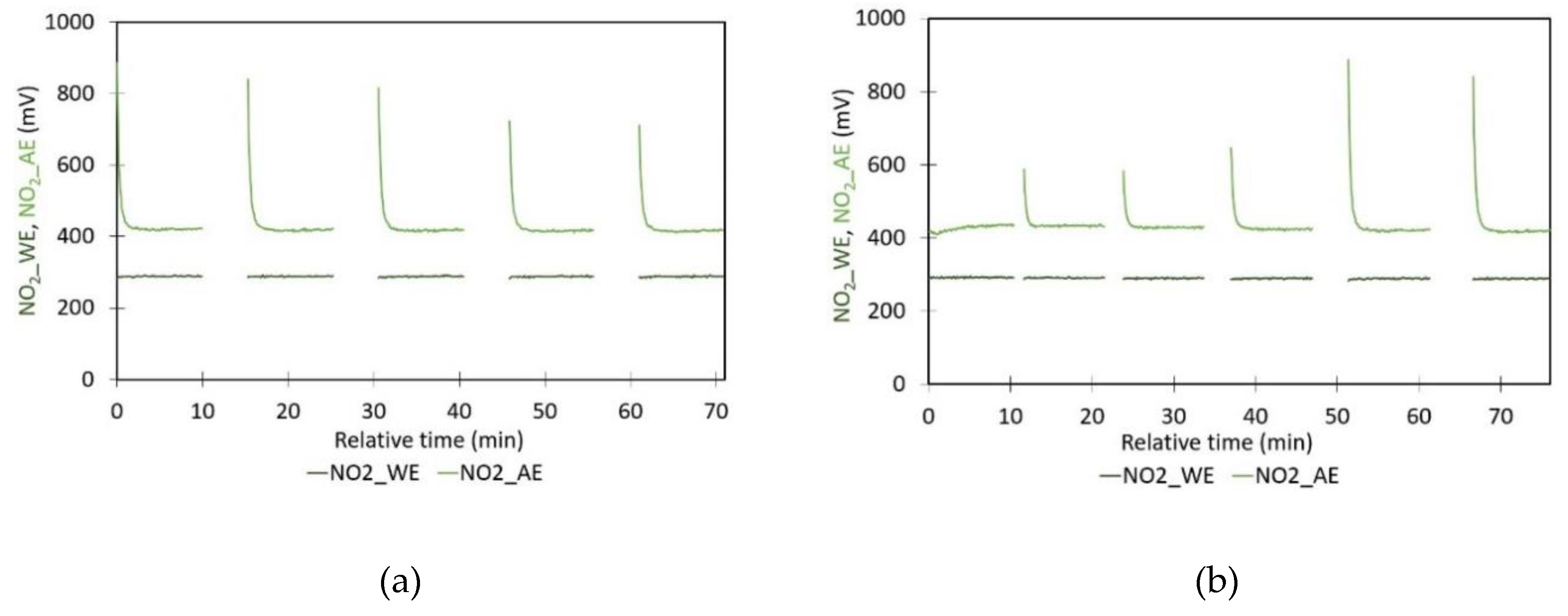
Figure 2.
WE and AE sensor signals of the NO2 sensor inside the calibration box in ambient air; a) Internal heater gradually increased above 50°C; a) External heater resulted in a slower increase in temperature above 40°C.
Figure 2.
WE and AE sensor signals of the NO2 sensor inside the calibration box in ambient air; a) Internal heater gradually increased above 50°C; a) External heater resulted in a slower increase in temperature above 40°C.
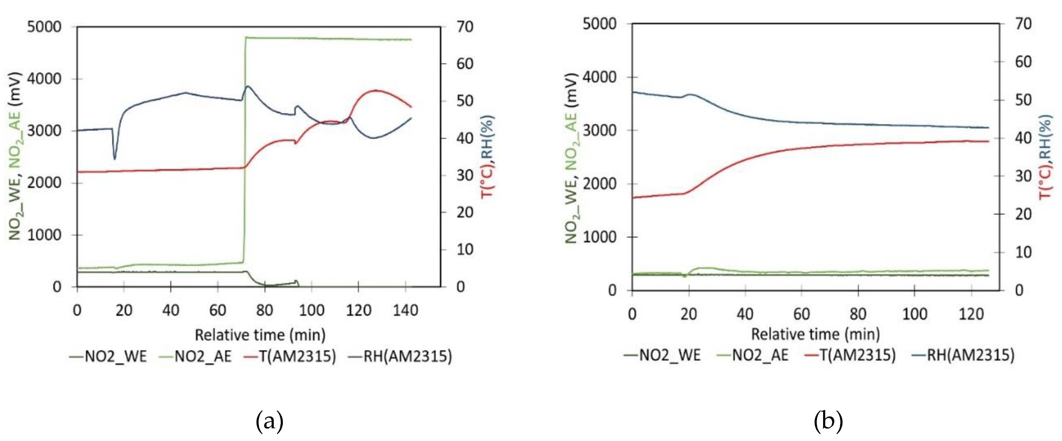
Figure 3.
Two different experiments at which the temperature inside the calibrated box at ambient air was increased during heating; a) Temperature of the mica heater controller was increased in steps of 1°C; b) The External heater caused a shock in the AE-signal despite the gradual increase in temperature.
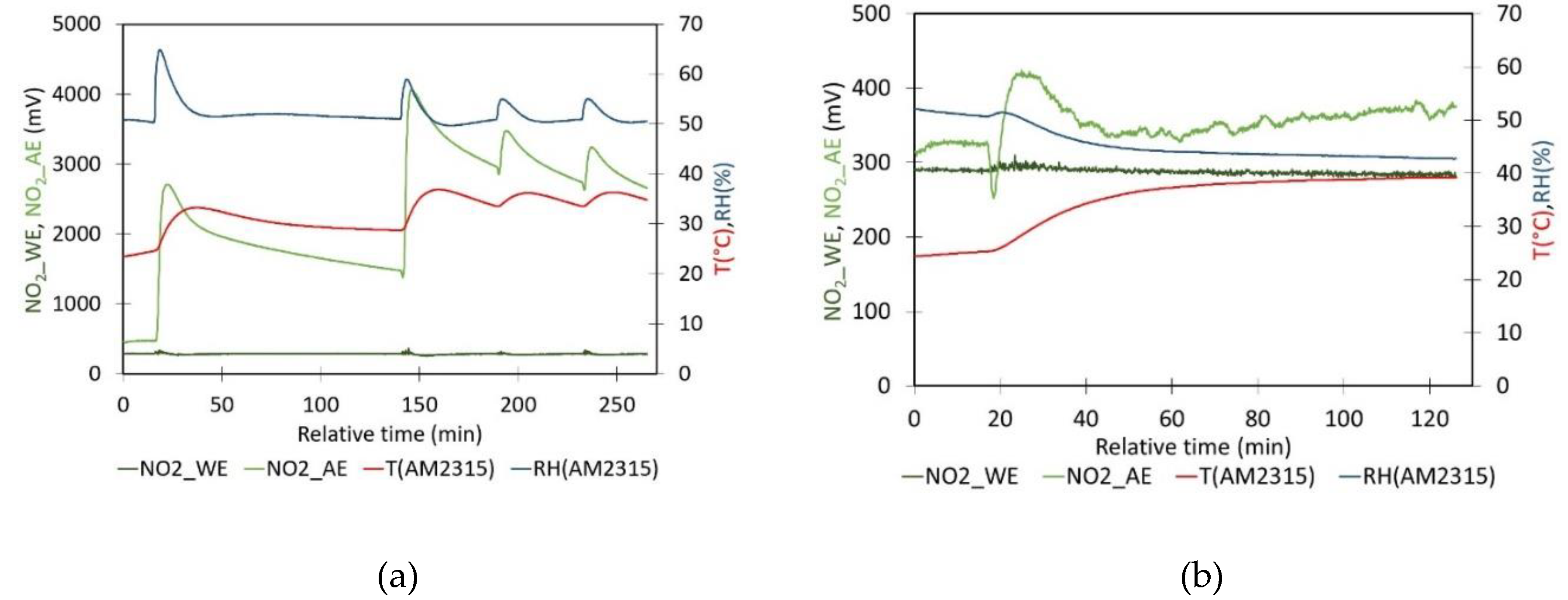
Figure 4.
Sensor signal of the NO2 sensor when 2,0 mL of pure NO2 gas is injected in the calibration box at 29°C and 54% of RH. The experiment started and ended in zero air.
Figure 4.
Sensor signal of the NO2 sensor when 2,0 mL of pure NO2 gas is injected in the calibration box at 29°C and 54% of RH. The experiment started and ended in zero air.
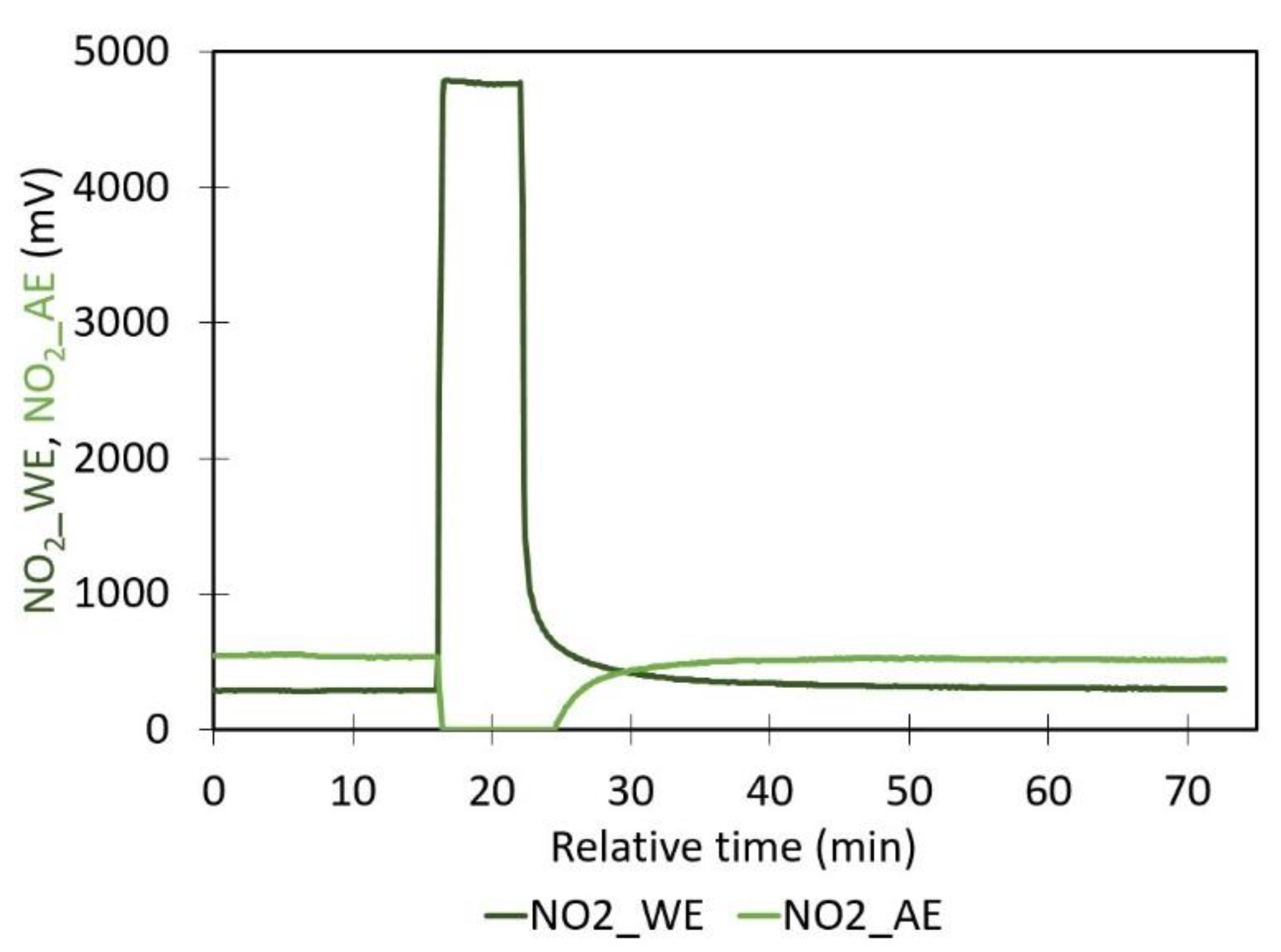
Figure 5.
Effect of Heating and cooling on nT in zero air; (a) Evolution of nT over time and the occurrence of hysteresis; (b) Average nT value for temperature intervals of 0.5°C for the temperature range between 14°C and 42°C.
Figure 5.
Effect of Heating and cooling on nT in zero air; (a) Evolution of nT over time and the occurrence of hysteresis; (b) Average nT value for temperature intervals of 0.5°C for the temperature range between 14°C and 42°C.
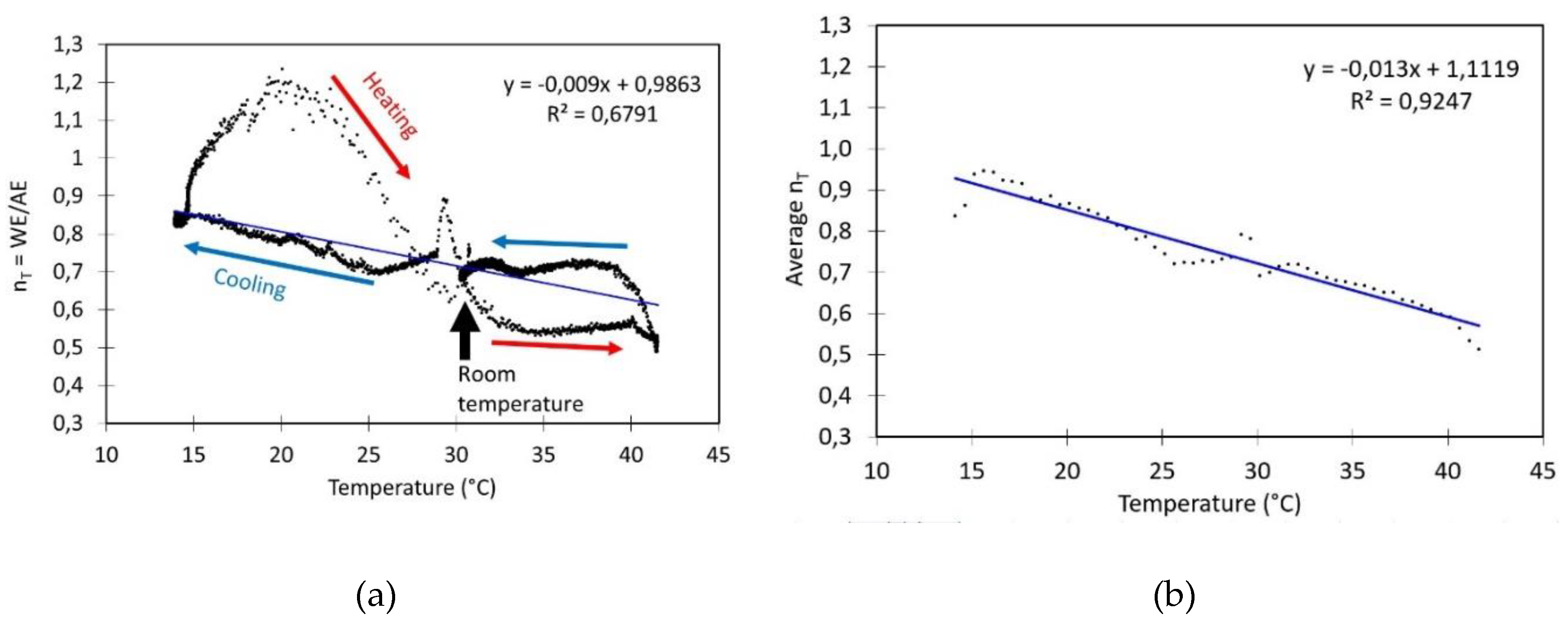
Figure 6.
Effect of T and RH on nT as RH varies in the calibration box filled with clean ambient air; (a) Evolution of nT with RH; (b) Evolution of nT with T during RH variation.
Figure 6.
Effect of T and RH on nT as RH varies in the calibration box filled with clean ambient air; (a) Evolution of nT with RH; (b) Evolution of nT with T during RH variation.
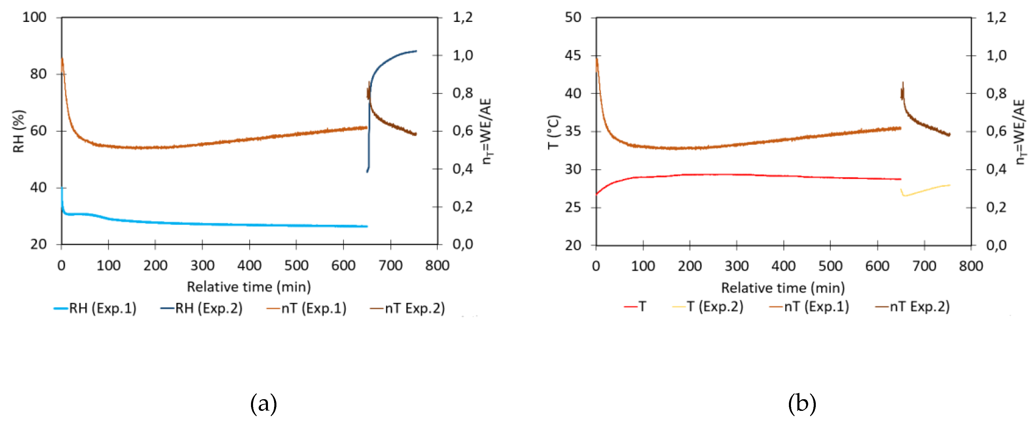
Figure 7.
Effect of the injection of known amounts of NO2 (a) on the sensor signals; (b) on WEgas.
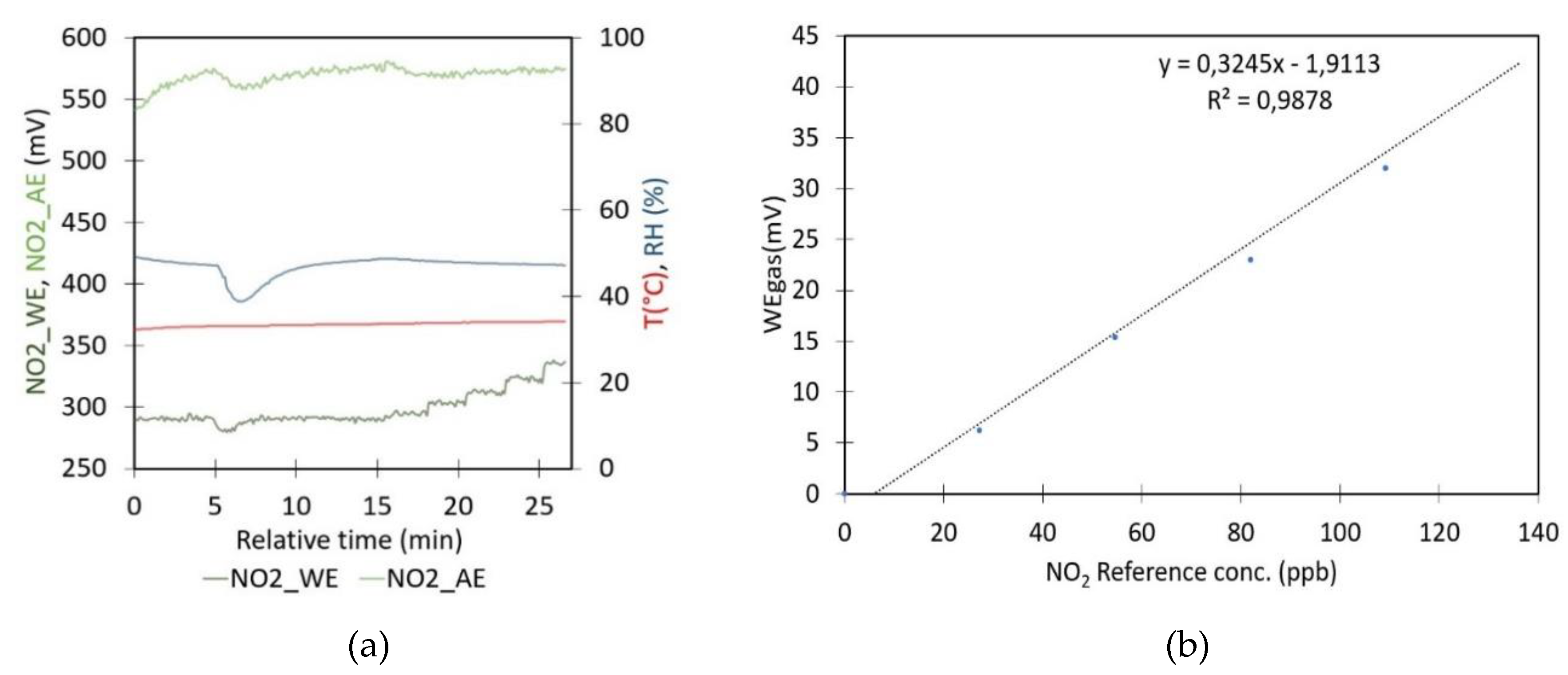

Table 1.
Overview of variables and their definitions.
| WE0 | The value of the working electrode in air in total absence of the target analyte (i.e., zero air) under fixed conditions, as specified in the calibration certificate provided by Alphasense, which is measured at a pressure of 101 kPa, a temperature of 23 ± 2°C, and a relative humidity of 40 ± 15%. |
| AE0 | The value of the auxiliary electrode in air in total absence of the target analyte (i.e., zero air) under fixed conditions, as specified in the calibration certificate provided by Alphasense, which is measured at a pressure of 101 kPa, a temperature of 23 ± 2°C, and a relative humidity of 40 ± 15%. |
| WEbackground | The value of the working electrode in zero air at any given moment during the monitoring campaign. This value is partially determined by the instantaneous temperature and relative humidity. These conditions may be different from the ones at which WE0 is determined. |
| AE | The measured value of the auxiliary electrode at any given moment. This value depends partly on the instantaneous temperature and relative humidity but is supposed to be independent of the concentration of the target analyte, since the electrode is not in direct contact with the sampled gas. However, the measuring conditions may deviate from those at which AE0 was originally measured. |
| WEgas | A portion of the total measured value WEtot that is linearly dependent on the concentration of the target analyte. |
| WEtot | The total measured value of the working electrode in ambient air reflects the combined contributions from the specific concentration of the target analyte at a given temperature and relative humidity WEgas, and the background interference WEbackground. |
Table 2.
The average and standard deviation of WE and AE are calculated for the last minute of each cycle after stabilization. Both experiments are conducted at an average temperature of 29°C and 50% RH. The drop rate is determined by calculating the difference between the first and last measurements.
| Cycle nr. | Experiment shown in Figure 1a | Experiment shown in Figure 1b | ||
| WE [mV] | AE [mV] | WE [mV] | AE [mV] | |
| 1 | 288.8 ± 1.2 | 420.5 ± 1.9 | 291.7 ± 1.3 | 432.6 ± 2.7 |
| 2 | 288.4 ± 1.1 | 418.0 ± 2.1 | 290.5 ± 1.0 | 433.2 ± 1.7 |
| 3 | 288.4 ± 1.2 | 417.2 ± 2.2 | 289.6 ± 1.1 | 428.5 ± 1.5 |
| 4 | 288.1 ± 1.4 | 416.2 ± 2.0 | 289.2 ± 1.3 | 423.5 ± 1.9 |
| 5 | 288.1 ± 1.3 | 415.9 ± 2.1 | 288.8 ± 1.2 | 420.3 ± 2.0 |
| 6 | - | - | 288.5 ± 1.1 | 417.8 ± 2.1 |
| Average | 288 ± 1 | 418 ± 3 | 290 ± 2 | 426 ± 6 |
| Drop [mV/h] | 0.38 | 2.5 | 2.7 | 12.7 |
Table 3.
Results of zero air measurements from various experiments conducted under different ambient conditions and at different times, ranked from highest to lowest temperatures.
Table 3.
Results of zero air measurements from various experiments conducted under different ambient conditions and at different times, ranked from highest to lowest temperatures.
| Experiment | T [°C] | RH [%] | WE [mV] | AE [mV] | nT |
| Temperature | 33 | 48 | 290 | 574 | 0.5065 |
| Cycle on/off | 29 | 50 | 288 | 418 | 0.6890 |
| RH exp. 1 | 28.9 | 26.7 | 276.5 | 472.6 | 0.5851 |
| RH exp.1 | 28.5 | 89.0 | 292.9 | 437.7 | 0.6692 |
| RH exp.2 | 27.0 | 27.1 | 281.8 | 501.78 | 0.5615 |
| RH exp.2 | 27.9 | 88.1 | 294.7 | 505.0 | 0.5835 |
| Alphasense | 23 ± 2 | 40 ± 15 | 289 | 290 | 0.9966 |
Disclaimer/Publisher’s Note: The statements, opinions and data contained in all publications are solely those of the individual author(s) and contributor(s) and not of MDPI and/or the editor(s). MDPI and/or the editor(s) disclaim responsibility for any injury to people or property resulting from any ideas, methods, instructions or products referred to in the content. |
© 2024 by the authors. Licensee MDPI, Basel, Switzerland. This article is an open access article distributed under the terms and conditions of the Creative Commons Attribution (CC BY) license (http://creativecommons.org/licenses/by/4.0/).
Copyright: This open access article is published under a Creative Commons CC BY 4.0 license, which permit the free download, distribution, and reuse, provided that the author and preprint are cited in any reuse.


