
Submitted:
04 October 2024
Posted:
07 October 2024
You are already at the latest version
Abstract
Approximate Computing (AxC) has emerged as a promising paradigm to enhance performance and energy efficiency by allowing a controlled trade-off between accuracy and resource consumption. It is extensively adopted across various abstraction levels, from software to architecture and circuit levels, employing diverse methodologies. The primary objective of AxC is to reduce energy consumption for executing error-resilient applications, accepting controlled and inherently acceptable output quality degradation. However, harnessing AxC poses several challenges, including identifying segments within a design amenable to approximation and selecting suitable AxC techniques to fulfill accuracy and performance criteria.
This survey provides a comprehensive review of recent methodologies proposed for performing Design Space Exploration (DSE) to find the most suitable AxC techniques, focusing on both hardware and software implementations. DSE is a crucial design process where system designs are modeled, evaluated, and optimized for various extra-functional system behaviors such as performance, power consumption, energy efficiency, and accuracy. A systematic literature review was conducted to identify papers that ascribe their DSE algorithms, excluding those relying on exhaustive search methods. This survey aims to detail the state-of-the-art DSE methodologies that efficiently select AxC techniques, offering insights into their applicability across different hardware platforms and use-case domains. For this purpose, papers were categorized based on the type of search algorithm used, with Machine Learning (ML) and Evolutionary Algorithms (EAs) being the predominant approaches. Further categorization is based on the target hardware, including Field-Programmable Gate Arrays (FPGAs), Application-Specific Integrated Circuits (ASICs), general-purpose Central Processing Units (CPUs), and Graphics Processing Units (GPUs). A notable observation was that most studies targeted image processing applications due to their tolerance for accuracy loss. By providing an overview of techniques and methods outlined in existing literature pertaining to the DSE of AxC designs, this survey elucidates the current trends and challenges in optimizing approximate designs.
Keywords:
Approximate Computing
; Design Space Exploration
; Circuit Design
; High Level Synthesis
; Multi-objective Optimization
1. Introduction
As large-scale application domains like scientific computing, social media, and financial analytics continue to expand, the computational and storage requirements of modern systems have surpassed the available resources. In the upcoming decade, it is anticipated that the amount of data managed by global data centers will increase by fifty times, while the number of processors will only grow by a factor of ten [1]. This indicates that the demand for performance will soon outstrip resource allocations.
Furthermore, Information and Communication Technology (ICT) devices and services currently contribute significantly to the world’s overall energy consumption, with projections indicating that their energy demand will rise to nearly 21% by 2030 [2] Consequently, it becomes evident that relying solely on over-provisioning resources will not suffice to address the impending challenges facing the computing industry.
In recent decades, significant technological advancements and increasing computational demands have driven a remarkable reduction in the size of integrated circuits and computing systems. This downscaling of CMOS technology has resulted in several key benefits, such as enhanced computational performance, improved energy efficiency, and the ability to increase the number of cores per chip. Smaller transistors allow for faster switching speeds, enabling higher clock frequencies, which translates to quicker data processing and more powerful computing systems. Additionally, as transistors shrink, the power required to switch them can be reduced, leading to lower overall energy consumption, which is crucial for mobile and battery-operated devices.
However, CMOS downscaling is not without its drawbacks. As transistors continue to shrink, the benefits of reduced supply voltage become less significant, and the leakage current (unwanted current that flows even when the transistor is off) becomes more pronounced, leading to higher static power consumption. Moreover, the exponential increase in power consumption due to higher clock frequencies has introduced thermal challenges, as more energy is dissipated as heat, which can damage the chip and reduce its lifespan. The combination of these factors means that the traditional benefits of CMOS scaling are diminishing, and the ability to further increase the number of cores per chip is constrained by power and thermal limits. Consequently, as CMOS technology reaches its scaling limits, it becomes imperative to explore alternative approaches, such as new materials, 3D stacking, or novel architectures, to continue improving computing efficiency without exacerbating these power and thermal issues [3].
In addition to the trends mentioned above, the nature of the tasks fueling the demand for computing has evolved across the computing spectrum, spanning from mobile devices to the cloud. Within data centers and the cloud, the impetus for computing stems from the necessity to efficiently manage, organize, search, and derive conclusions from vast datasets. In contrast, the predominant computing demand for mobile and embedded devices arises from the desire for more immersive media experiences and more natural, intelligent interactions with users and the surrounding environment. Although computational errors are generally undesirable, a common thread runs through this spectrum: these applications are not primarily concerned with computing precise numerical outputs. Instead, "correctness" is defined as generating results that are sufficiently accurate to deliver an acceptable user experience [4].
These applications inherently possess a resilience towards errors, meaning they can produce satisfactory outputs even when some of their computations are carried out in an approximate manner [5]. For instance, in search and recommendation systems, there is not always a single definitive or "golden" result; instead, multiple answers falling within a specific range are considered acceptable. Additionally, iterative applications processing extensive data sets may terminate convergence prematurely or employ heuristics [6]. In many machine learning applications, even if a golden result exists, the most advanced algorithms may not be able to achieve it. Consequently, users often have to settle for results that are reasonably inaccurate but still adequate. Furthermore, applications such as multimedia, wireless communication, speech recognition, and data mining exhibit a degree of tolerance toward errors. Human perceptual limitations signify that such errors may not significantly affect applications like image, audio, and video processing. Another example pertains to applications dealing with noisy input data (e.g., image and sensor data processing, and speech recognition). The noise in the input naturally leads to imprecise results, and approximations have a similar impact. In simpler terms, applications that can handle noisy inputs also possess the capability to withstand approximations [7,8,9]. Finally, some applications utilize computational patterns like aggregation or iterative refinement, which can mitigate or compensate for the effects of approximations.
An encouraging approach to enhance computing efficiency is AxC. The concept of AxC encompasses a wide array of techniques that capitalize on the inherent error resilience of applications, ultimately leading to improved efficiency across all layers of the computing stack, ranging from the fundamental transistor-level design to software implementations. These techniques can have varying impacts on both the hardware and the quality of the output. AxC capitalizes on the existence of data and algorithms that can tolerate errors, as well as the limitations in the perception of end-users. It strategically balances accuracy against the potential for performance improvements or energy savings. In essence, it takes advantage of the gap that often exists between the level of accuracy that computer systems can provide and the level of accuracy required by the specific application or the end-users. This required accuracy is typically much lower than what the computer systems can deliver.
Leveraging AxC involves addressing a few aspects and challenges. The first challenge is identifying the segments within the targeted software or hardware component that can be candidates for approximation. Identifying segments of code or data that can be approximated may necessitate a comprehensive understanding of the application on behalf of the designer.
The second challenge is implementing the AxC technique to introduce approximations. On the one hand, there is a limit to the accuracy degradation that can be introduced so the output remains acceptable. On the other hand, the level of accuracy degradation and the performance improvements or energy savings varies depending on the selected AxC technique. Hence, available AxC techniques should be evaluated and compared to find the most suitable AxC technique tailored for a target application or design.
The next challenge is choosing the suitable error measurement criteria, often tailored to the particular application, and executing the actual error assessment process to ensure that the output adheres to the predefined quality standards [5]. The error assessment usually involves simulating both the precise and approximate versions of applications. However, alternative methods like Bayesian inference [10,11] or Machine Learning (ML)-based approaches [12] have been put forth in the scientific literature.
A DSE can be performed to address all the previously mentioned challenges. The goal of performing a DSE is to determine the most optimal approximate configurations from those generated by applying a given set of approximation techniques to the design. Hence, the DSE approaches can help systematically evaluate different approximate designs to choose the most suitable AxC techniques and, consequently, the best configurations for any given combination of AxC techniques. Early DSE approaches either combine multiple design objectives into a single-objective optimization problem or optimize a solitary parameter while keeping the remaining variables constant. More recent research, as seen in published works, has tackled circuit design issues by considering a mop to seek out Pareto-optimal approximate circuit configurations [13]. Regrettably, these approaches predominantly concentrated on simple systems, specifically arithmetic components like adders and multipliers, as they form the foundational components for more intricate designs [14].
This paper aims to cover different DSE approaches leveraged in comparing approximate versions of a target application or design. The structure of this paper is as follows: Firstly, Section 2 provides a background on the AxC techniques and DSE approaches. Then, in Section 3, the search methodology to find related studies and categorizing them, is explained. In Section 4 DSE approaches to compare and choose suitable AxC techniques are reviewed and compared. Finally, a conclusion is provided in Section 5.
2. Background
AxC represents an emerging paradigm enabling the development of significantly energy-efficient computing systems, including diverse hardware accelerators designed for tasks like image filtering, video processing, and data mining. This approach leverages the inherent error resilience of many applications, allowing for a trade-off between accuracy and energy efficiency [15]. This trade-off can be accomplished through various means, spanning from transistor-level design to software implementations, each with distinct effects on hardware integrity and output quality.
The following sections provide an overview of how different AxC techniques can be classified, followed by a description of the DSE paradigm.
2.1. Classification of Approximate Computing Techniques
AxC techniques can be classified into three groups based on their implementation level: software, architecture, and hardware, with specific techniques applicable at multiple levels, as shown in Figure 1. For instance, memory read approximation can be achieved through pure software approaches or within memory control units. While Figure 1 highlights some commonly utilized approximation methods from the existing literature, it is essential to note that there exist numerous ways to approximate an application, and the precise definition of what constitutes an approximation is a subject of debate [9,16].
2.1.1. Software-Level Approximate Computing Techniques
The loop-perforation technique serves as a notable example of software approximation, enabling the generation of valuable outcomes without executing every iteration of an iterative code [17]. Similarly, function-skipping involves bypassing specific code blocks during runtime based on predefined conditions [18,19,20]. Another software approximation method involves reducing the bit-width used for data representation, primarily impacting the memory footprint of the application. While reducing data precision can also affect the execution time and performance of the software, its impact relies on the hardware implementation of operations utilized by the application [21,22].
Memoization is a technique that optimizes performance and conserves energy by storing previously computed values for specific inputs. When the same input is re-encountered later, the stored value is reused, eliminating the need for redundant computation. This trade-off between computation and memory use enhances efficiency and reduces resource consumption [23].
2.1.2. Architectural-Level Approximate Computing Techniques
nn can learn the behavior of a standard function implementation by analyzing how it responds to various inputs. Through software-hardware co-design, traditional code can be transformed into nn with lower output accuracy but enhanced execution time and performance [29].
Memory access skipping combines memoization and function skipping techniques to omit uncritical memory accesses without significant accuracy loss. Approximate nn leverage this approach to skip reading entire weight matrix rows for non-critical neurons, reducing energy consumption and improving performance [30].
2.1.3. Circuit and Hardware-Level Approximate Computing Techniques
Voltage scaling techniques reduce energy consumption in digital circuits by adjusting the supply voltage at the circuit level. This adjustment directly impacts computation timing and power efficiency, exploiting the inherent error resilience of applications to achieve significant energy savings while maintaining acceptable performance levels [31]. Dynamic Voltage Scaling (DVS) adjusts the supply voltage to decrease power dissipation while maintaining computational accuracy within safe operational limits, balancing power savings against performance degradation [32]. Dynamic Voltage and Frequency Scaling (DVFS) extends this concept by simultaneously adjusting both the voltage and the operating frequency, providing finer control over power and performance trade-offs [31]. In contrast, Voltage Over Scaling (VOS) aggressively reduces the supply voltage beyond nominal levels, intentionally allowing timing violations that can introduce errors in computations [33,34]. While DVS and DVFS ensure accurate results within controlled performance constraints, VOS prioritizes further energy savings by permitting computational inaccuracies, making it suitable for scenarios where approximate results are acceptable.
Hardware-based approximation techniques often employ alternative implementations of arithmetic operators. For instance, variable approximation modes on operators represent one such approach. Hardware approximation also finds application in the image processing domain through approximate compressors [9,16].
Inexact hardware can provide approximation at the hardware level, with numerous examples from the literature of approximate arithmetic circuits designed to balance performance and accuracy. Adders, multipliers, and dividers significantly influence performance and energy efficiency across various computing tasks since they are the most frequent and vital arithmetic components within a processor. Pursuing enhanced speed, power efficiency, and error resilience in numerous applications such as multimedia processing, recognition systems, and data analytics has propelled the advancement of approximate arithmetic design [3].
The aforementioned AxC techniques are a few examples of the many approximation techniques implemented at various abstraction levels. Due to this complexity, the challenges mentioned in the previous section need to be addressed, and DSE emerges as the most promising solution thus far.
2.2. Precision Metrics
Various precision metrics have been proposed to describe and evaluate the effectiveness of AxC techniques and methodologies, as detailed in Table 1.
Error Distance (ED) and Error Probability (EP) are basic error metrics used for measuring the accuracy degradation while applying AxC techniques. ED is the distance between the correct output and the approximate output of a circuit for each scenario and EP is the probability of having a wrong answer which is calculated by the number of wrong answers over the number of all input scenarios. These metrics are formulated in equations (1) and (2) respectively.
where N is the number of possible scenarios, and are the accurate and approximate outputs of scenario respectively, and is the probability of the scenario happening.
Mean Error Distance (MED) is the average of all the error distances which is calculated as equation (3).
Mean Relative Error Distance (MRED) is the average of error distances relative to the correct answers formulated as equation (4).
Absolute Worst-Case Error (AWCE) which is defined as the largest error distance that can happen, formulated in equation (5).
Mean Squared Error (MSE) is the average of the squares of the errors between the approximate values and the accurate values. MSE is formulated as equation (6).
Hamming Distance (HD) is a metric used to measure the difference between two strings of equal length. It is defined as the number of positions at which the corresponding symbols are different. For example, consider the binary strings "1011101" and "1001001". The HD is 2 because there are two positions where the strings differ (second and fourth positions).
Error Rate (ER) measures the number of erroneous results over the total number of results. In equation (7), represents the number of erroneous results, while the represents the total number of results.
Bit Error Ratio (BER) is the number of bit errors per unit of time, calculated by dividing the number of bit errors by the total number of bits transferred during a given time interval. BER is a unitless performance measure and is often expressed as a percentage. It is a critical metric for evaluating the accuracy and reliability of data transmission in communication systems. In equation (8), represents the number of erroneous bits, while the represents the total number of bits.
Peak Signal-to-Noise Ratio (PSNR) is a metric that evaluates the quality of reconstructed images or videos by comparing them to their originals. It measures the ratio between the maximum possible signal power and the power of corrupting noise, expressed in decibels (dB). Higher PSNR values indicate better quality. PSNR is formulated as equation (9) where R is the maximum possible pixel value (e.g., 255 for an 8-bit image), and corresponds to the MSE between the original and the distorted image.
Structural Similarity Index Measure (SSIM) measures image quality by comparing structural information, luminance, and contrast between an image and a reference. Unlike PSNR, SSIM focuses on perceptual similarity. SSIM values range from -1 to 1, with 1 indicating perfect similarity. SSIM is defined in equation (10), where x and y are the two images being compared. The parameters and represent the mean pixel values of images x and y, respectively. and are the variances of x and y, while denotes the covariance between the two images. The constants and are included to stabilize the division, particularly when the denominators approach zero, and are typically defined as and , where L is the dynamic range of pixel values (e.g., 255 for 8-bit images), and and are small constants (commonly set to 0.01 and 0.03, respectively).
Mean Pixel Difference (MPD) is a simpler metric that calculates the average absolute difference in pixel values between two images. Lower MPD values indicate higher similarity. MPD is formulated as equation (11), where N is the number of pixels, is the original pixel value, and is the compared pixel value.
Binary classification is widely used in applied machine learning across fields like medicine, biology, meteorology, and malware analysis. Performance metrics are crucial in research to evaluate and report the effectiveness of classification models. In binary classification, a two-by-two confusion matrix captures the model’s performance, consisting of tp, tn, fp, and fn. Key metrics such as classification accuracy, precision, and recall are derived from these values [35].
Classification accuracy is the proportion of correct classifications out of all classifications, both positive and negative. Classification accuracy is formulated as equation (12) and reflects the overall correctness of the classifier. A perfect model has an accuracy of 1.0 (or 100%), meaning no fp or fn.
Recall or tp rate is the proportion of actual positives that were correctly identified. This metric is formulated in (13) and measures the model’s ability to detect all positive instances. A perfect recall is 1.0, indicating a 100% detection rate with no fn.
False positive rate (FPR), also known as the probability of false alarm, is the proportion of actual negatives that were incorrectly classified as positives. This metric is formulated in equation (14) and indicates the likelihood of misclassifying a negative instance as positive. A perfect model has an False Positive Rate (FPR) of 0.0 (or 0%), meaning no fp.
The precision metric is the proportion of correct positive classifications. This metric is formulated in equation (15). Precision assesses the accuracy of the positive predictions made by the model. A perfect precision score is 1.0, achieved when there are no fp. While Precision improves as fp decrease, Recall improves as fn decrease.
2.3. Design Space Exploration
DSE is a systematic process of analyzing and evaluating various design alternatives to find optimal solutions that meet specific requirements and constraints. In the context of embedded system design and AxC, DSE can be defined as systematically evaluating and analyzing various design alternatives to find optimal solutions that balance performance, power consumption, and accuracy trade-offs. The goal of DSE is to find the best approximate versions of an application or circuit that provide significant gains in efficiency (power, speed, area) while maintaining acceptable output quality for the target application [37,38].
Designing modern embedded computer systems presents numerous formidable challenges, as these systems typically must adhere to various strict and sometimes conflicting design criteria. Embedded systems aimed at mass production and battery-powered or passive-cooling devices require cost-effectiveness and energy efficiency. In safety-critical applications like avionics and space technologies, dependability is paramount, especially with the growing autonomy of systems. Furthermore, many of these systems are expected to support multiple applications and standards simultaneously, necessitating real-time performance. For instance, mobile devices must accommodate various communication protocols and digital content coding standards [39].
Additionally, these systems must offer flexibility for future updates and extensions while maintaining programmability despite the necessity of implementing significant portions in dedicated hardware blocks due to performance, power consumption, and cost constraints. Consequently, modern embedded systems often adopt a heterogeneous multi-processor architecture comprising a mix of programmable cores and dedicated hardware blocks for time-sensitive tasks. This trend has led to the development of integrated heterogeneous Multi-Processor System-on-Chip (MPSoC) architectures [40].
To address the intricate design challenges inherent in such systems, a new design methodology known as system-level design has emerged over the past 15 to 20 years [41]. Its primary objective is to elevate the level of abstraction in the design process, thereby enhancing design productivity. Central to this approach are MPSoC platform architectures, which facilitate the reuse of IP components, along with the concept of high-level system modeling and simulation [42,43].
High-level system modeling and simulation enable the representation of platform components and their interactions at a refined level of abstraction. These models streamline the modeling effort, optimize execution speed, and are thus invaluable for early-stage DSE. Various design alternatives can be examined during DSE, including the number and type of processors utilized, the interconnection network employed, and the spatial and temporal binding of application tasks to processor cores [44,45].
Initiating DSE at the early stages of the design process is crucial, as the choices made can significantly impact the success or failure of the final product. However, the challenges the large design space poses, particularly in its early stages, cannot be overlooked. For instance, when considering different mappings of application tasks to processing resources to optimize system performance or power consumption, the design space expands exponentially with the number of tasks and processors, presenting an NP-hard problem [46]. Consequently, notable research has focused on developing efficient and effective DSE methods in recent years, aiming to tackle the complexities of exploring such expansive design spaces [46].
DSE approaches can be categorized and classified based on many aspects [47]. However, one of the possible classifications is categorizing a DSE as single-objective or multi-objective. Multi-objective DSE refers to simultaneously optimizing multiple conflicting objectives or goals during the design phase. These objectives typically include performance, power consumption, area utilization, reliability, and cost in circuit design. Unlike single-objective optimization, where a single criterion is optimized at the expense of others, multi-objective DSE aims to find a set of trade-off solutions, known as the Pareto-optimal front, where improving one objective comes at the cost of degrading another. That is why finding an optimal solution that optimizes all objectives is impossible. Such a solution does not exist, and this happens when the objectives conflict with each other. Therefore, optimal decisions need to be taken with trading-off between design criteria. [45].
When applying AxC techniques to the design, what makes choosing among different AxC techniques difficult is that all of them can be employed together, requiring the evaluation of the impact of each combination of AxC techniques on the overall computation accuracy. The two main approaches for evaluating this impact comprise executing different approximated versions of the application several times with different configurations [48,49] or devising modeling techniques to simulate different approximated versions of the application in a time-optimized fashion [50,51]. The disadvantage of the first approach is that the evaluation time increases when the exploration reaches an exhaustive search. Applying pruning techniques to the exploration space reduces the exploration time to the application execution time, at best. Conversely, the second approach is more suitable for estimating the impact of AxC techniques on the application computation accuracy because it is faster than the first approach, even though it costs an error margin in the computation accuracy evaluation.
3. Literature Search Methodology
The objective of this survey was to systematically identify and classify existing literature on DSE methodologies proposed for finding the most suitable AxC techniques to be applied to a program or hardware design.
The initial search focused on identifying papers that provided a detailed description of the algorithms used for DSE. To maintain a high standard of relevance, only studies that clearly explained their DSE methodologies were included. Papers that utilized exhaustive search methods were deliberately excluded, as the survey aimed to highlight more sophisticated and efficient approaches.
Once the relevant papers were identified, they were categorized based on the type of search algorithm employed for conducting the DSE. Within each category, the papers were further sorted based on the target hardware for which the DSE was conducted. For instance, some studies focus on fpga and asic, particularly in the context of designing accelerators using AxC techniques. Some other studies do not specify a particular target hardware, indicating their proposed methods can be applied universally across different platforms. Additionally, some papers address hardware or software level approximation for gpu.
This survey also considers the application domains of the programs targeted for approximation. The application domains usually considered in most studies for selecting benchmarks include image processing, signal processing, scientific computing, financial analysis, Natural Language Processing (NLP), 3D gaming, and robotics.
Additionally, information about employed AxC techniques was extracted from each study to better compare different studies based on the AxC techniques applied at software, architectural, or hardware levels.
In a nutshell, this survey aimed to identify and evaluate the proposed DSE methods employed to explore the extensive design space of approximate versions of a design. The focus was on understanding whether these methods were well-known search algorithms or custom approaches. Following this structured and systematic methodology, the survey provides a comprehensive overview of the current state-of-the-art proposed DSE methodologies for finding the most suitable AxC techniques, highlighting the diversity of approaches and their applicability to various hardware platforms and application domains. Figure 2 shows the aforementioned process of categorizing different studies.
4. Comparison and Analysis
This section provides an overview and comparison of the proposed DSE approaches in the literature for applying AxC techniques to programs or hardware designs. Though many different search algorithms have been proposed in the literature to explore the vast design space of approximate programs or hardware designs, two categories of algorithms are commonly leveraged: ML algorithms and ea. ML approaches often leverage data-driven techniques to predict and explore optimal design configurations, while ea use bio-inspired strategies such as ga to navigate the design space.
Table 2 provides information about the research works that took an ML approach to perform the DSE, while Table 3 includes information about the research works that leveraged ea to perform the DSE. All the remaining research works that perform the DSE using other heuristic algorithms or combining different optimization algorithms are listed in Table 4 and Table 5. While Table 2, Table 3, Table 4, Table 5, and Table 6 provide an overview to allow comparison among different studies based on the employed search algorithm, target hardware, and use case domain, Table 7, Table 8, Table 9, Table 10, and Table 11 provide an overview of the same sets of studies to allow comparison among different studies based on AxC techniques applied in each study.
As reported in Table 2, the most popular ML algorithm is RL [38,52,56,57]. While [53] and [54] use MBO and modified MCTS, respectively; [12,55] mention using ML based search algorithm. Among these research works, though the target hardware varies from fpga and asic to general-purpose cpu, the use-case domain always includes image and signal processing benchmarks, ranging from traditional image processing to image classification using nn. Moving the comparison to the AxC techniques applied at different levels, as reported in Table 7, replacing the exact adders and multipliers with approximate counterparts is the most common hardware-level approximation investigated [12,38,53,54,55]. However, the investigated software-level AxC techniques are noticeably application-specific: In [52,53], algorithm parameters - that indicate the iterations of executing a code basic block or the size of the inputs processed at each iteration - are decreased to reduce the execution time or program memory while sacrificing output accuracy. A similar approach of loop perforation is applied in [56] alongside changing the input data structure. Interestingly, in [57], an ML algorithm is employed to search the design space of an ML application, proposing a DSE framework to find the optimal quantization level for each layer of a dnn.
Table 3 lists the research works that leveraged ea to perform the DSE. Between the prominently used subsets of ea, an es algorithm is only used in [60]. all approaches enlisted here, either use ga or its subset NSGA-II to explore the design space. More precisely, [58,59,62] employ ga, [60,61] use NSGA-II, and [63] developed a NAS algorithm based on NSGA-II. Comparing the target hardware of the reviewed research works, most works consider optimizing an accelerator design for fpga and asic implementation as expected, while [63] targets gpu for optimizing cnn designs.
Comparing the benchmarks in Table 3 to those listed in Table 2, most of the benchmarks fall under the image processing category, though the types of benchmarks are slightly different. Comparing the applied AxC techniques, as reported in Table 8,58,59] investigate employing sparse lut, precision scaling, and approximate adders for a pixel-streaming pipeline application accelerated with an fpga. Similarly, [60,61] explore using approximate adders and multipliers for optimizing video and image compression accelerators. In [62], authors try to optimize benchmarks from different domains such as scientific computing, 3D gaming, 3D image rendering, signal, and image processing when the approximation is applied at a software level, altering the program static instructions. Distinctively, in [63], authors propose approximating multipliers using lut and a customized approximate convolutional layer to support quantization-aware training of cnn and dynamically explore the design space. It is noteworthy that the aim is to optimize a cnn design usually trained on a gpu. Hence, approximation at the hardware level is not an option, while such AxC technique can be emulated at the software level.
Table 4 and Table 5 report a list of reviewed papers that neither rely on ML nor ea to explore the design space. In [70], authors mention using a TS algorithm, with potential integration of ga into the DSE framework. Notably, TS focuses on iteratively improving a single solution, whereas ga work with a population of solutions and evolve them over generations using crossover, mutation, or other genetic operators. Hence, taking a TS approach might not seem the best choice when the mop does not have a single optimum solution, and a Pareto Front of non-dominated solutions may represent the optima better. In [72], authors select a GD approach to search the design space. Contrary to the fact that GD is a widely used optimization technique in ML, GD is not employed as a part of an ML search algorithm in the aforementioned work. All the remaining works in Table 4 and Table 5 employ custom algorithms. In some cases, the DSE includes multiple stages of exploration, where pruning techniques are used before applying the search algorithm to reduce the design space size or after applying the search algorithm to refine the obtained solution sets.
Table 4 categorizes studies by target hardware, starting with those focused on fpga and asic, and continues through Table 5 with studies on optimized accelerator design. Table 9 and Table 10 report the AxC techniques applied in each study enlisted in Table 4 and Table 5. Similar to the other sets of studies presented in Table 2 and Table 3, only a few works reported in Table 4 and Table 5 are hardware-independent or target general-purpose cpu and gpu. The target hardware in [64] includes both fpga and asic. In [64], the DSE is performed to optimize a hardware accelerator design for a video processing application using approximate adders and logic blocks. Similarly, in [65], the target hardware includes both fpga and asic. In this study, the DSE is performed to optimize the design of dnn accelerated using fpga and asic, while the AxC techniques applied are quantization techniques aimed at approximating the dnn design at the software level. [66], performs the DSE with a heuristic search algorithm to optimize the hardware implementation of different functions used in a dnn vector accelerator. To apply approximation through logic isolation, the portions of logic in the circuit that consume significant power but contribute only minimally to output accuracy are identified. Then the DSE is performed to find the best trade-off between dnn classification accuracy and energy savings. It can be implied that the target hardware can be categorized as asic. In [67,68], the DSE is performed with custom algorithms, applying hardware approximations to hardware implementations of video and image processing benchmarks. The target hardware in these studies can be categorized as asic. In [69,70], the authors propose to modify the HLS tools to study the approximation effects.
Continuing through Table 5,71] performs the DSE to optimize hardware accelerator design, investigating both hardware level and software level approximation techniques. Other three works also perform the DSE to optimize the accelerator design, specifically for ML applications [72,73,74]. In [75], authors target a very different type of acceleration using npu. While the use of npu for acceleration purposes can be categorized as applying approximation at the architectural level, the target hardware can be classified in the asic category. Though in [76], the target hardware is not explicitly mentioned; the proposed methodology applies to any DSE performed on general-purpose cpu as target hardware. In [77], authors perform the DSE to find the best configuration when applying their proposed hardware level approximation technique which is specific to gpu. However, the approximation technique is also applied to some benchmarks executed on general-purpose cpu to provide a fair comparison between the results obtained by performing the DSE for both hardware targets.
Comparing the use case domains across Table 4 and Table 5, image and signal processing are the prevalent categories of applications. Moreover, ML applications for image and text classification, pattern and speech recognition, and NLP tasks are considered in many works. Some works also target image compression tasks. Many works include matrix multiplication, DCT, FIR, and Sobel filters in their studies, as these functions are crucial for many image-processing tasks. Some works also consider benchmarks from financial analysis, robotics, 3D gaming, and scientific computing domains.
Considering the AxC techniques mentioned in Table 9 and Table 10, studies in [64,67,70,71,76] investigate using approximate adders and multipliers. In [66], authors propose applying a hardware-level AxC technique called logic isolation using latches or AND/OR gates at the inputs, MUXes at the output, and power gating. In [68], authors propose applying another hardware-level AxC technique called Clock-gating, alongside the precision reduction of primary inputs at the RTL level. Similarly, [72] proposes to apply a Clock Overgating technique. In [71], authors propose to use VOS alongside approximate adders and multipliers at the hardware level, while approximating the additions and multiplications also on the software level. In [69], authors propose very different AxC techniques: Internal Signal Substitution, and Bit-Level Optimization at the RTL level, Functional Unit Substitution (additions and multiplications) at the HLS level, and Source-Code Pruning Based on Profiling at the software level. Also, in [73,74], authors propose applying AxC techniques at multiple levels while designing an AI accelerator. They propose applying precision reduction to dnn data, as well as using approximated versions of fundamental dnn functions such as activation functions, pooling, normalization, and data shuffling in the network accelerator design. Though also aiming at optimizing dnn designs, authors in [65] propose to apply AxC techniques at the software level to enable dynamic quantization of the dnn during the training phase. Interestingly, in [75], authors propose to use a very different AxC technique compared to all of these reviewed studies. The proposed approach includes approximating the entire program using an npu as an accelerator. Another interesting AxC technique is proposed in [77] to tackle memory bottlenecks while executing the program on a gpu and transferring the data from cpu to gpu and vice versa.
Some studies in the literature propose approaches to efficiently explore the design space for approximate logic synthesis and consider approximate versions of circuits generated by approximating selected portions (or sub-functions) of Boolean networks. These studies are reported separately in Table 6, while the applied AxC techniques in these studies are reported in Table 11. The approximation is applied at the hardware level and involves logic falsification in [78,80]. The approximation technique in [79] is based on Boolean network simplifications allowed by exdc. The approximation in [81] is based on BMF for truth tables. And, in [82], a customized approximation of Boolean networks is applied. The search algorithm to explore the design space is an NSGA-II in [78,80,82] while in [79,81] authors employ customized and heuristic algorithms. While the benchmarks for all of these studies include well-known approximate adders and multipliers in the literature, other circuits such as ALUs, decoders, shifters, and multiple combinational circuits have been employed as benchmarks. Interestingly, in [80], the study targets safety-critical applications. The Quadruple Approximate Modular Redundancy (QAMR) approach is opposed to Triple Modular Redundancy (TMR), where all modules are exact circuits.
While Table 2, Table 3, Table 4, Table 5, and Table 6 provide an overview to allow comparison among different studies based on employed search algorithm, target hardware, use case domain, Table 12, Table 13, Table 14, Table 15, and Table 16 provide an overview of the same sets of studies to allow comparison among different studies based on evaluated parameters involved in the trade-off imposed by approximation.
Since AxC trades off accuracy for performance and energy efficiency, the first important parameter to evaluate during DSE is accuracy. Depending on the approximation goals, parameters measured during DSE in different studies may vary.
Predictably, power consumption is a key parameter frequently targeted in the reviewed studies, as it directly impacts energy efficiency. However, many studies choose to target energy consumption instead of power consumption. This approach is entirely valid because energy savings inherently indicate power savings, considering that energy is the product of power and time. By measuring energy directly, these studies effectively capture the combined impact of power reduction and execution time, providing a comprehensive view of the gains in efficiency achieved through AxC techniques.
The second most in-demand parameter, especially when designing accelerators, is the circuit area. Understandably, when approximations are applied to optimize a design, specifically in the case of employing the design on fpga, reducing the area utilization or LUT count is one of the approximation goals.
After area, performance and execution time are the most commonly measured parameters. In applications such as ann, where execution time is inherently high, one of the primary goals of applying approximation is to reduce this execution time, particularly for inference and, when feasible, training. The lengthy execution times of these applications also directly impact the DSE time, as evaluating even a few approximate instances can become highly time-consuming. While typical application execution times may range from seconds to minutes, the DSE time needed to explore and evaluate possible approximations often extends to hours or days. In the case of ann, the execution time for inference alone can take hours, and the DSE time required to assess even a limited number of approximate instances can span several days. Therefore, in applications where the execution time is already considerable and hence a primary target to trade-off with accuracy, proposing DSE methodologies that can assess more approximate instances in a reasonable time becomes crucial.
Memory utilization is often the least frequently evaluated parameter in the reviewed studies. Many AxC techniques are primarily applied to optimize execution time, energy, or performance, rather than specifically targeting memory utilization. However, these techniques can still impact memory utilization. For instance, some techniques aimed at reducing execution time, energy consumption, or improving performance may also affect memory usage as a secondary outcome. This indirect influence on memory is an important consideration, even though it is not the primary focus of these techniques. For example, in [52] authors propose to explore the design space comprised of approximate versions of an iris scanning pipeline. The approximation includes reducing the search window size and the region of interest in iris images, reducing the parameters of iris segmentation, and reducing the kernel size of the filter. Though the main target is to reduce program execution time, the memory needed to store the intermediate and final output images and program parameters is reduced. In [77], authors propose an AxC technique to mitigate the bottlenecks of limited off-chip bandwidth and long access latency, when the data is transferred from cpu to gpu and back. When a cache miss happens, RFVP predicts the requested values. In this case, the main goal of approximation is to achieve off-chip memory bandwidth consumption reduction, while speedup and energy reductions are also reported.
Through Table 12, Table 13, Table 14, Table 15, and Table 16, besides the accuracy column, there is an error metric(s) column that reports the error metric(s) presented in each study to measure accuracy degradation due to applying approximation. Among all the parameters mentioned - power consumption, execution time, performance, memory utilization, and circuit area - accuracy is unique because the metrics used to measure accuracy degradation are often more complex and application-specific. For example, while power consumption differences are reported simply as ED between the measurements from approximate and exact versions, accuracy degradation error metrics involve a variety of sophisticated measures that are tailored to the specific application domain. In Table 1, the most popular error metrics are listed.
Finally, every proposed DSE approach results in a solution or a set of optimal solutions for the mop. In some cases, an optimal solution exists. In many other cases, no global optimal solution can be found, and a Pareto Front (a set of non-dominated solutions) is presented. The last column in Table 12, Table 13, Table 14, Table 15, and Table 16 indicates the studies that reported a Pareto Front as the result of the DSE performed, or at least compared a set of solutions resulted from the proposed DSE approach with a Pareto Front obtained by exhaustive search or other methods. In most cases, the obtained Pareto Front shows a trade-off between accuracy on the one hand, and an evaluated parameter such as energy efficiency, on the other hand, [12,52,53,54,56,58,59,60,61,63,67,68,69,70,71,78,79,80,81,82].
The rest of the reviewed studies that did not obtain a Pareto Front but provided other analysis methods for comparing the DSE results are considered hereafter.
In some studies, a single threshold or multiple thresholds for the acceptable accuracy degradation was set, and then the DSE was performed for each accuracy threshold. For example, in [55], a solution was provided for each accuracy threshold. In [64], performance is plotted for different accelerator designs. However, no Pareto front is provided. Also, in [66], three different dnn accuracy thresholds were set, and the DSE was performed for each threshold. Hence, the plots show the energy reductions for each dnn accuracy threshold instead of a Pareto front. Similarly, in [72], the plots show the energy reductions for each dnn accuracy threshold instead of a Pareto front.
In [57], two application-specific error metrics were proposed to evaluate the accuracy for dnn quantization and plot the quantization space Pareto frontier for these two error metrics called State of Relative Accuracy and State of Quantization.
In [38], an RL approach was selected for performing the DSE, and steps of exploration have been plotted for evaluated parameters, including accuracy; however, a Pareto front is not obtained. In [62], plots show the accuracy and energy against multiple thresholds for the number of program instructions to be approximated. However, a comparison to the Pareto front is not provided.
In [65], the quantization is applied dynamically during training and inference of the dnn. Therefore, the plots show the changes in the dnn accuracy concerning the number of MACs used in the computations. Also, in the same plot, the results are compared to other quantization-aware approaches in the literature instead of comparing the results with a Pareto front obtained by other DSE methods. Since in dynamic approximation of the dnn, the changes in accuracy during the training or inference are more representative of the approach effectiveness, plotting a Pareto front seems unnecessary.
In [73] and the previous studies with the same framework [74], no Pareto front was presented. Instead, for each dnn, compute efficiency, training throughput, and inference latency were reported. In [75], an npu is employed as an accelerator for a frequently executed region of code or function to approximate the function by replacing it with a neural network. Since an ann is employed, similar to other works on ann, multiple thresholds for function quality loss, or in other words, different ann accuracy levels, were investigated. Hence, the speedup and energy reduction for multiple thresholds of function quality loss were plotted. In consequence, no Pareto front was demonstrated.
5. Conclusion
This survey systematically reviewed and classified existing literature on DSE methodologies aimed at identifying suitable AxC techniques for various applications and hardware designs. The search strategy focused on papers that provided detailed descriptions of their DSE algorithms, deliberately excluding those utilizing exhaustive search methods to highlight more sophisticated and efficient approaches.
Two dominant categories of DSE methods emerged from the reviewed studies: ML approaches and ea methods. While both methodologies have strengths, the relative advantages depend largely on the complexity of the design space and the target application.
The ML approaches, especially those leveraging RL, are highly effective in domains like image processing and dnn, where the design space is structured, and substantial data from previous executions is available. These approaches excel at fine-tuning trade-offs between power and accuracy dynamically, making them suitable for applications requiring frequent reconfigurations or those with domain-specific training data [52,57]. However, ML-based DSE methods tend to be more application-specific and less adaptable to broader hardware platforms or large, complex design spaces [53,54].
In contrast, ea-based methods, particularly those utilizing ga and NSGA-II, offer greater flexibility and scalability. These methods are especially suited for complex design spaces like fpga, asic, and other hardware-specific optimizations. ga have been proven to deliver robust, Pareto-optimal solutions across a variety of applications, including image and video processing, where they consistently outperform other approaches in balancing circuit area, power consumption, and execution time [58,61]. Moreover, NSGA-II has shown particular promise in optimizing dnn, delivering effective performance-power trade-offs nn accelerator designs [63].
In conclusion, while ML-based DSE approaches offer fine-tuned control and are highly effective in specialized applications, ea-based DSE methods, especially ga, are better suited for complex and large-scale design spaces that require general-purpose optimization. Future research may combine the adaptability of ea-based DSE approaches with the fine-grained control of ML-based methods, creating hybrid models that can optimize across diverse hardware environments and application domains.
Author Contributions
S.S. and A.P. contributed to the conceptualization, design, and methodology of the study. S.S. performed the literature review and analysis, while A.P. assisted in drafting and refining the manuscript. Both authors engaged in discussions regarding the findings and conclusions of the survey. B.D., I.O., A.B., A.S., and S.D. contributed to supervision, paper writing, project administration, and funding acquisition.
Funding
This paper has received funding from:
Institutional Review Board Statement
Not applicable.
Informed Consent Statement
Not applicable.
Data Availability Statement
Not applicable.
Conflicts of Interest
The authors declare no conflicts of interest. The funders had no role in the design of the study; in the collection, analyses, or interpretation of data; in the writing of the manuscript; or in the decision to publish the results.
References
- Mittal, S. A survey of techniques for approximate computing. ACM Computing Surveys (CSUR) 2016, 48, 1–33. [Google Scholar] [CrossRef]
- Jones, N. How to stop data centres from gobbling up the world’s electricity. Nature 2018, 561, 163–166. [Google Scholar] [CrossRef] [PubMed]
- Jiang, H.; Liu, C.; Liu, L.; Lombardi, F.; Han, J. A Review, Classification, and Comparative Evaluation of Approximate Arithmetic Circuits. J. Emerg. Technol. Comput. Syst. 2017, 13. [Google Scholar] [CrossRef]
- Venkataramani, S.; Chakradhar, S.T.; Roy, K.; Raghunathan, A. Approximate computing and the quest for computing efficiency. 2015 52nd ACM/EDAC/IEEE Design Automation Conference (DAC), 2015, pp. 1–6. [CrossRef]
- Chippa, V.K.; Chakradhar, S.T.; Roy, K.; Raghunathan, A. Analysis and characterization of inherent application resilience for approximate computing. Proceedings of the 50th Annual Design Automation Conference, 2013, pp. 1–9.
- Esmaeilzadeh, H.; Sampson, A.; Ceze, L.; Burger, D. Neural Acceleration for General-Purpose Approximate Programs. 2012 45th Annual IEEE/ACM International Symposium on Microarchitecture, 2012, pp. 449–460. [CrossRef]
- Han, J.; Orshansky, M. Approximate computing: An emerging paradigm for energy-efficient design. 2013 18th IEEE European Test Symposium (ETS), 2013, pp. 1–6. [CrossRef]
- Traiola, M.; Virazel, A.; Girard, P.; Barbareschi, M.; Bosio, A. Testing approximate digital circuits: Challenges and opportunities. 2018 IEEE 19th Latin-American Test Symposium (LATS), 2018, pp. 1–6. [CrossRef]
- Bosio, A.; Ménard, D.; Sentieys, O. (Eds.) Approximate Computing Techniques; Springer International Publishing, 2022. [CrossRef]
- Traiola, M.; Savino, A.; Barbareschi, M.; Di Carlo, S.; Bosio, A. Predicting the impact of functional approximation: From component-to application-level. 2018 IEEE 24th International Symposium on On-Line Testing And Robust System Design (IOLTS). IEEE, 2018, pp. 61–64.
- Traiola, M.; Savino, A.; Di Carlo, S. Probabilistic estimation of the application-level impact of precision scaling in approximate computing applications. Microelectronics Reliability 2019, 102, 113309. [Google Scholar] [CrossRef]
- Mrazek, V.; Hanif, M.A.; Vasicek, Z.; Sekanina, L.; Shafique, M. autoax: An automatic design space exploration and circuit building methodology utilizing libraries of approximate components. Proceedings of the 56th Annual Design Automation Conference 2019, 2019, pp. 1–6. [Google Scholar]
- Sekanina, L.; Vasicek, Z.; Mrazek, V. Automated search-based functional approximation for digital circuits. Approximate Circuits: Methodologies and CAD.
- Barbareschi, M.; Barone, S.; Mazzocca, N.; Moriconi, A. Design Space Exploration Tools. In Approximate Computing Techniques: From Component-to Application-Level; Springer, 2022; pp. 215–259.
- Xu, Q.; Mytkowicz, T.; Kim, N.S. Approximate computing: A survey. IEEE Design & Test 2015, 33, 8–22. [Google Scholar]
- Rodrigues, G.; Lima Kastensmidt, F.; Bosio, A. Survey on Approximate Computing and Its Intrinsic Fault Tolerance. Electronics 2020, 9. [Google Scholar] [CrossRef]
- Li, S.; Park, S.; Mahlke, S. Sculptor: Flexible approximation with selective dynamic loop perforation. Proceedings of the 2018 International Conference on Supercomputing, 2018, pp. 341–351.
- Goiri, I.; Bianchini, R.; Nagarakatte, S.; Nguyen, T.D. Approxhadoop: Bringing approximations to mapreduce frameworks. Proceedings of the Twentieth International Conference on Architectural Support for Programming Languages and Operating Systems, 2015, pp. 383–397.
- Vassiliadis, V.; Parasyris, K.; Chalios, C.; Antonopoulos, C.D.; Lalis, S.; Bellas, N.; Vandierendonck, H.; Nikolopoulos, D.S. A programming model and runtime system for significance-aware energy-efficient computing. ACM SIGPLAN Notices 2015, 50, 275–276. [Google Scholar] [CrossRef]
- Raha, A.; Venkataramani, S.; Raghunathan, V.; Raghunathan, A. Quality configurable reduce-and-rank for energy efficient approximate computing. 2015 Design, Automation & Test in Europe Conference & Exhibition (DATE). IEEE, 2015, pp. 665–670.
- Rubio-González, C.; Nguyen, C.; Nguyen, H.D.; Demmel, J.; Kahan, W.; Sen, K.; Bailey, D.H.; Iancu, C.; Hough, D. Precimonious: Tuning assistant for floating-point precision. Proceedings of the international conference on high performance computing, networking, storage and analysis, 2013, pp. 1–12.
- Hsiao, C.C.; Chu, S.L.; Chen, C.Y. Energy-aware hybrid precision selection framework for mobile GPUs. Computers & Graphics 2013, 37, 431–444. [Google Scholar]
- Sinha, S.; Zhang, W. Low-Power FPGA Design Using Memoization-Based Approximate Computing. IEEE Transactions on Very Large Scale Integration (VLSI) Systems 2016, 24, 2665–2678. [Google Scholar] [CrossRef]
- Sampaio, F.; Shafique, M.; Zatt, B.; Bampi, S.; Henkel, J. Approximation-aware multi-level cells STT-RAM cache architecture. 2015 International Conference on Compilers, Architecture and Synthesis for Embedded Systems (CASES). IEEE, 2015, pp. 79–88.
- Tian, Y.; Zhang, Q.; Wang, T.; Yuan, F.; Xu, Q. ApproxMA: Approximate memory access for dynamic precision scaling. Proceedings of the 25th edition on Great Lakes Symposium on VLSI, 2015, pp. 337–342.
- Ranjan, A.; Venkataramani, S.; Fong, X.; Roy, K.; Raghunathan, A. Approximate storage for energy efficient spintronic memories. Proceedings of the 52nd Annual Design Automation Conference, 2015, pp. 1–6.
- Shafique, M.; Ahmad, W.; Hafiz, R.; Henkel, J. A low latency generic accuracy configurable adder. Proceedings of the 52nd Annual Design Automation Conference; Association for Computing Machinery: New York, NY, USA, 2015. [Google Scholar] [CrossRef]
- Venkataramani, S.; Chakradhar, S.T.; Roy, K.; Raghunathan, A. Approximate computing and the quest for computing efficiency. Proceedings of the 52nd Annual Design Automation Conference, 2015, pp. 1–6.
- St Amant, R.; Yazdanbakhsh, A.; Park, J.; Thwaites, B.; Esmaeilzadeh, H.; Hassibi, A.; Ceze, L.; Burger, D. General-purpose code acceleration with limited-precision analog computation. ACM SIGARCH Computer Architecture News 2014, 42, 505–516. [CrossRef]
- Zhang, Q.; Wang, T.; Tian, Y.; Yuan, F.; Xu, Q. ApproxANN: An approximate computing framework for artificial neural network. 2015 Design, Automation & Test in Europe Conference & Exhibition (DATE). IEEE, 2015, pp. 701–706.
- Mohapatra, D.; Chippa, V.K.; Raghunathan, A.; Roy, K. Design of voltage-scalable meta-functions for approximate computing. 2011 Design, Automation & Test in Europe, 2011, pp. 1–6. [CrossRef]
- Kumar, V.I.; Kapat, S. Per-Core Configurable Power Supply for Multi-Core Processors with Ultra-Fast DVS Voltage Transitions. 2022 IEEE Applied Power Electronics Conference and Exposition (APEC), 2022, pp. 1028–1034. [CrossRef]
- Senobari, A.; Vafaei, J.; Akbari, O.; Hochberger, C.; Shafique, M. A Quality-Aware Voltage Overscaling Framework to Improve the Energy Efficiency and Lifetime of TPUs based on Statistical Error Modeling. IEEE Access 2024. [Google Scholar] [CrossRef]
- Chatzitsompanis, G.; Karakonstantis, G. On the Facilitation of Voltage Over-Scaling and Minimization of Timing Errors in Floating-Point Multipliers. 2023 IEEE 29th International Symposium on On-Line Testing and Robust System Design (IOLTS), 2023, pp. 1–7. [CrossRef]
- Seliya, N.; Khoshgoftaar, T.M.; Van Hulse, J. A study on the relationships of classifier performance metrics. 2009 21st IEEE international conference on tools with artificial intelligence. IEEE, 2009, pp. 59–66.
- Leon, V.; Hanif, M.A.; Armeniakos, G.; Jiao, X.; Shafique, M.; Pekmestzi, K.; Soudris, D. Approximate computing survey, Part II: Application-specific & architectural approximation techniques and applications. arXiv preprint arXiv:2307.11128, arXiv:2307.11128 2023.
- Schafer, B.C.; Wang, Z. High-level synthesis design space exploration: Past, present, and future. IEEE Transactions on Computer-Aided Design of Integrated Circuits and Systems 2019, 39, 2628–2639. [Google Scholar] [CrossRef]
- Saeedi, S.; Savino, A.; Di Calro, S. Design Space Exploration of Approximate Computing Techniques with a Reinforcement Learning Approach. 2023 53rd Annual IEEE/IFIP International Conference on Dependable Systems and Networks Workshops (DSN-W). IEEE, 2023, pp. 167–170.
- Pimentel, A.D., Methodologies for Design Space Exploration. In Handbook of Computer Architecture; Chattopadhyay, A., Ed.; Springer Nature Singapore: Singapore, 2022; pp. 1–31. [CrossRef]
- Wolf, W.; Jerraya, A.A.; Martin, G. Multiprocessor system-on-chip (MPSoC) technology. IEEE transactions on computer-aided design of integrated circuits and systems 2008, 27, 1701–1713. [Google Scholar] [CrossRef]
- Santos, L.; Rigo, S.; Azevedo, R.; Araujo, G. Electronic System Level Design. In Electronic System Level Design: An Open-Source Approach; Rigo, S., Azevedo, R., Santos, L., Eds.; Springer Netherlands: Dordrecht, 2011; pp. 3–10. [Google Scholar] [CrossRef]
- Keutzer, K.; Newton, A.R.; Rabaey, J.M.; Sangiovanni-Vincentelli, A. System-level design: Orthogonalization of concerns and platform-based design. IEEE transactions on computer-aided design of integrated circuits and systems 2000, 19, 1523–1543. [Google Scholar] [CrossRef]
- Sangiovanni-Vincentelli, A.; Martin, G. Platform-based design and software design methodology for embedded systems. IEEE Design & Test of computers 2001, 18, 23–33. [Google Scholar]
- Gries, M. Methods for evaluating and covering the design space during early design development. Integration 2004, 38, 131–183. [Google Scholar] [CrossRef]
- Pimentel, A.D. Exploring exploration: A tutorial introduction to embedded systems design space exploration. IEEE Design & Test 2016, 34, 77–90. [Google Scholar]
- Singh, A.K.; Shafique, M.; Kumar, A.; Henkel, J. Mapping on multi/many-core systems: Survey of current and emerging trends. Proceedings of the 50th Annual Design Automation Conference, 2013, pp. 1–10.
- Palar, P.S.; Dwianto, Y.B.; Zuhal, L.R.; Morlier, J.; Shimoyama, K.; Obayashi, S. Multi-objective design space exploration using explainable surrogate models. Structural and Multidisciplinary Optimization 2024, 67, 38. [Google Scholar] [CrossRef]
- Smithson, S.C.; Yang, G.; Gross, W.J.; Meyer, B.H. Neural networks designing neural networks: Multi-objective hyper-parameter optimization. 2016 IEEE/ACM International Conference on Computer-Aided Design (ICCAD), 2016, pp. 1–8. [CrossRef]
- Dupuis, E.; Novo, D.; O’Connor, I.; Bosio, A. On the Automatic Exploration of Weight Sharing for Deep Neural Network Compression. 2020 Design, Automation Test in Europe Conference Exhibition (DATE), 2020, pp. 1319–1322. [CrossRef]
- Traiola, M.; Savino, A.; Di Carlo, S. Probabilistic estimation of the application-level impact of precision scaling in approximate computing applications. Microelectronics Reliability 2019, 102, 113309. [Google Scholar] [CrossRef]
- Savino, A.; Traiola, M.; Carlo, S.D.; Bosio, A. Efficient Neural Network Approximation via Bayesian Reasoning. 2021 24th International Symposium on Design and Diagnostics of Electronic Circuits Systems (DDECS), 2021, pp. 45–50. [CrossRef]
- Hashemi, S.; Tann, H.; Buttafuoco, F.; Reda, S. Approximate computing for biometric security systems: A case study on iris scanning. 2018 Design, Automation & Test in Europe Conference & Exhibition (DATE). IEEE, 2018, pp. 319–324.
- Ullah, S.; Sahoo, S.S.; Kumar, A. Clapped: A design framework for implementing cross-layer approximation in fpga-based embedded systems. 2021 58th ACM/IEEE Design Automation Conference (DAC). IEEE, 2021, pp. 475–480.
- Rajput, M.A.; Alyami, S.; Ahmed, Q.A.; Alshahrani, H.; Asiri, Y.; Shaikh, A. Improved Learning-Based Design Space Exploration for Approximate Instance Generation. IEEE Access 2023, 11, 18291–18299. [Google Scholar] [CrossRef]
- Awais, M.; Ghasemzadeh Mohammadi, H.; Platzner, M. LDAX: a learning-based fast design space exploration framework for approximate circuit synthesis. Proceedings of the 2021 on Great Lakes Symposium on VLSI, 2021, pp. 27–32.
- Hoffmann, H. Jouleguard: Energy guarantees for approximate applications. Proceedings of the 25th Symposium on Operating Systems Principles, 2015, pp. 198–214.
- Elthakeb, A.T.; Pilligundla, P.; Mireshghallah, F.; Yazdanbakhsh, A.; Esmaeilzadeh, H. Releq: A reinforcement learning approach for automatic deep quantization of neural networks. IEEE micro 2020, 40, 37–45. [Google Scholar] [CrossRef] [PubMed]
- Manuel, M.; Kreddig, A.; Conrady, S.; Doan, N.A.V.; Stechele, W. Model-based design space exploration for approximate image processing on FPGA. 2020 IEEE Nordic Circuits and Systems Conference (NorCAS). IEEE, 2020, pp. 1–7.
- Kreddig, A.; Conrady, S.; Manuel, M.; Stechele, W. A Framework for Hardware-Accelerated Design Space Exploration for Approximate Computing on FPGA. 2021 24th Euromicro Conference on Digital System Design (DSD). IEEE, 2021, pp. 1–8.
- Prabakaran, B.S.; Mrazek, V.; Vasicek, Z.; Sekanina, L.; Shafique, M. Xel-FPGAs: An End-to-End Automated Exploration Framework for Approximate Accelerators in FPGA-Based Systems. 2023 IEEE/ACM International Conference on Computer Aided Design (ICCAD). IEEE, 2023, pp. 1–9.
- Barbareschi, M.; Barone, S.; Bosio, A.; Han, J.; Traiola, M. A Genetic-algorithm-based Approach to the Design of DCT Hardware Accelerators. ACM Journal on Emerging Technologies in Computing Systems (JETC) 2022, 18, 1–25. [Google Scholar] [CrossRef]
- Park, J.; Ni, K.; Zhang, X.; Esmaeilzadeh, H.; Naik, M. Expectation-oriented framework for automating approximate programming. Workshop on Approximate Computing Across the System Stack (WACAS), 2014.
- Pinos, M.; Mrazek, V.; Vaverka, F.; Vasicek, Z.; Sekanina, L. Acceleration techniques for automated design of approximate convolutional neural networks. IEEE Journal on Emerging and Selected Topics in Circuits and Systems 2023, 13, 212–224. [Google Scholar] [CrossRef]
- Shafique, M.; Hafiz, R.; Rehman, S.; El-Harouni, W.; Henkel, J. Cross-layer approximate computing: From logic to architectures. Proceedings of the 53rd Annual Design Automation Conference, 2016, pp. 1–6.
- Fu, Y.; You, H.; Zhao, Y.; Wang, Y.; Li, C.; Gopalakrishnan, K.; Wang, Z.; Lin, Y. Fractrain: Fractionally squeezing bit savings both temporally and spatially for efficient dnn training. Advances in Neural Information Processing Systems 2020, 33, 12127–12139. [Google Scholar]
- Jain, S.; Venkataramani, S.; Raghunathan, A. Approximation through logic isolation for the design of quality configurable circuits. 2016 Design, Automation & Test in Europe Conference & Exhibition (DATE). IEEE, 2016, pp. 612–617.
- Paim, G.; Rocha, L.M.G.; Amrouch, H.; da Costa, E.A.C.; Bampi, S.; Henkel, J. A cross-layer gate-level-to-application co-simulation for design space exploration of approximate circuits in HEVC video encoders. IEEE Transactions on Circuits and Systems for Video Technology 2019, 30, 3814–3828. [Google Scholar] [CrossRef]
- Alan, T.; Gerstlauer, A.; Henkel, J. Cross-layer approximate hardware synthesis for runtime configurable accuracy. IEEE Transactions on Very Large Scale Integration (VLSI) Systems 2021, 29, 1231–1243. [Google Scholar] [CrossRef]
- Xu, S.; Schafer, B.C. Exposing approximate computing optimizations at different levels: From behavioral to gate-level. IEEE Transactions on Very Large Scale Integration (VLSI) Systems 2017, 25, 3077–3088. [Google Scholar] [CrossRef]
- Castro-Godínez, J.; Mateus-Vargas, J.; Shafique, M.; Henkel, J. AxHLS: Design space exploration and high-level synthesis of approximate accelerators using approximate functional units and analytical models. Proceedings of the 39th International Conference on Computer-Aided Design, 2020, pp. 1–9.
- Zervakis, G.; Xydis, S.; Soudris, D.; Pekmestzi, K. Multi-level approximate accelerator synthesis under voltage island constraints. IEEE Transactions on Circuits and Systems II: Express Briefs 2018, 66, 607–611. [Google Scholar] [CrossRef]
- Kim, Y.; Venkataramani, S.; Roy, K.; Raghunathan, A. Designing approximate circuits using clock overgating. Proceedings of the 53rd Annual Design Automation Conference, 2016, pp. 1–6.
- Venkataramani, S.; Srinivasan, V.; Wang, W.; Sen, S.; Zhang, J.; Agrawal, A.; Kar, M.; Jain, S.; Mannari, A.; Tran, H. ; others. RaPiD: AI accelerator for ultra-low precision training and inference. 2021 ACM/IEEE 48th Annual International Symposium on Computer Architecture (ISCA). IEEE, 2021, pp. 153–166.
- Venkataramani, S.; Sun, X.; Wang, N.; Chen, C.Y.; Choi, J.; Kang, M.; Agarwal, A.; Oh, J.; Jain, S.; Babinsky, T.; others. Efficient AI system design with cross-layer approximate computing. Proceedings of the IEEE 2020, 108, 2232–2250. [Google Scholar] [CrossRef]
- Mahajan, D.; Yazdanbakhsh, A.; Park, J.; Thwaites, B.; Esmaeilzadeh, H. Towards statistical guarantees in controlling quality tradeoffs for approximate acceleration. ACM SIGARCH Computer Architecture News 2016, 44, 66–77. [Google Scholar] [CrossRef]
- Savino, A.; Portolan, M.; Leveugle, R.; Di Carlo, S. Approximate computing design exploration through data lifetime metrics. 2019 IEEE European Test Symposium (ETS). IEEE, 2019, pp. 1–7.
- Yazdanbakhsh, A.; Pekhimenko, G.; Thwaites, B.; Esmaeilzadeh, H.; Mutlu, O.; Mowry, T.C. RFVP: Rollback-free value prediction with safe-to-approximate loads. ACM Transactions on Architecture and Code Optimization (TACO) 2016, 12, 1–26. [Google Scholar] [CrossRef]
- Echavarria, J.; Wildermann, S.; Teich, J. Approximate logic synthesis of very large boolean networks. 2021 Design, Automation & Test in Europe Conference & Exhibition (DATE). IEEE, 2021, pp. 1552–1557.
- Miao, J.; Gerstlauer, A.; Orshansky, M. Multi-level approximate logic synthesis under general error constraints. 2014 IEEE/ACM International Conference on Computer-Aided Design (ICCAD). IEEE, 2014, pp. 504–510.
- Traiola, M.; Echavarria, J.; Bosio, A.; Teich, J.; O’Connor, I. Design Space Exploration of Approximation-Based Quadruple Modular Redundancy Circuits. 2021 IEEE/ACM International Conference On Computer Aided Design (ICCAD). IEEE, 2021, pp. 1–9.
- Ma, J.; Hashemi, S.; Reda, S. Approximate logic synthesis using boolean matrix factorization. IEEE Transactions on Computer-Aided Design of Integrated Circuits and Systems 2021, 41, 15–28. [Google Scholar] [CrossRef]
- Echavarria, J.; Keszocze, O.; Teich, J. Probability-based dse of approximated lut-based fpga designs. 2022 IEEE 15th Dallas Circuit And System Conference (DCAS). IEEE, 2022, pp. 1–5.
Figure 1.
A classification of the AxC techniques.
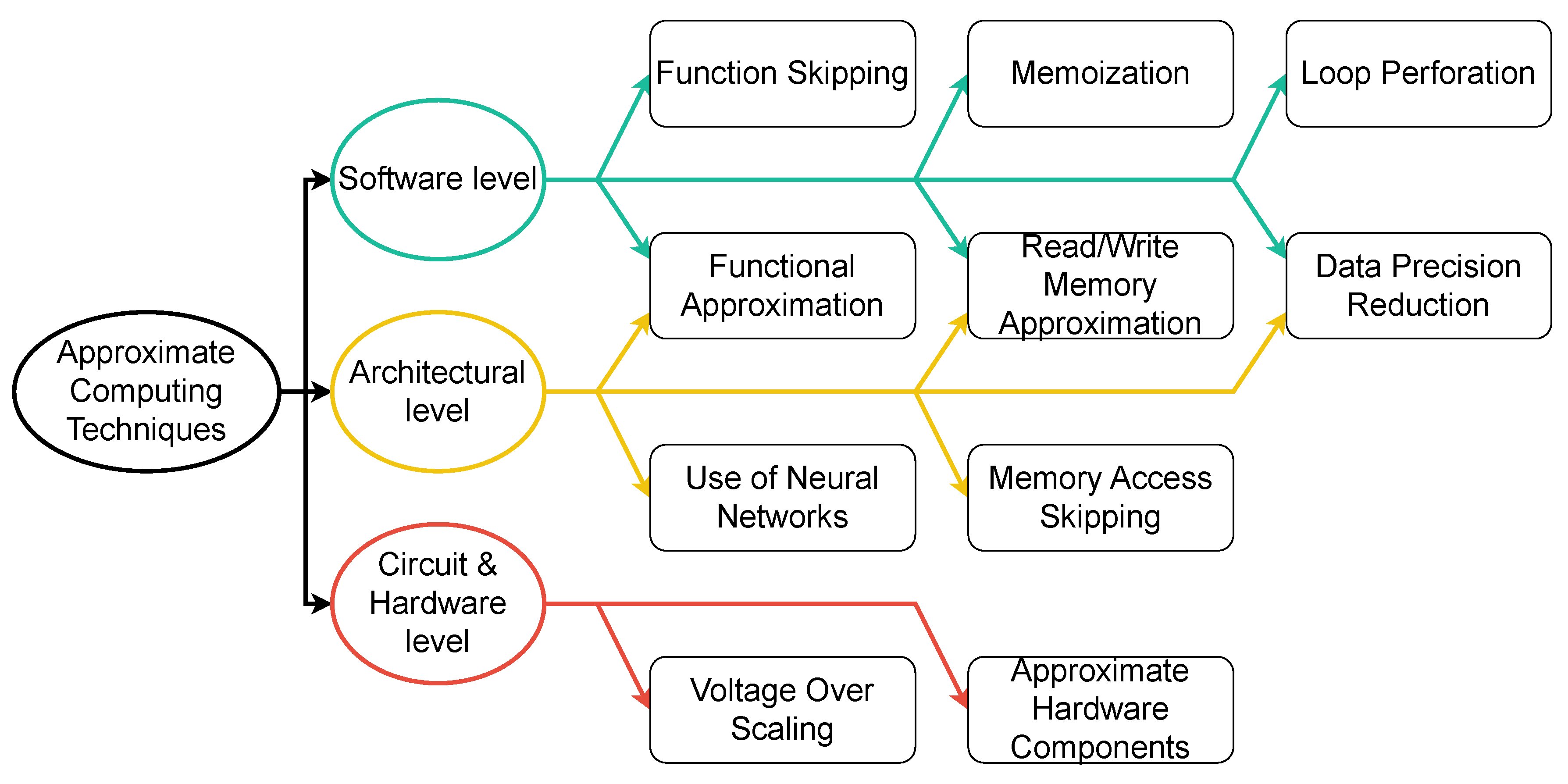
Figure 2.
Literature search methodology.
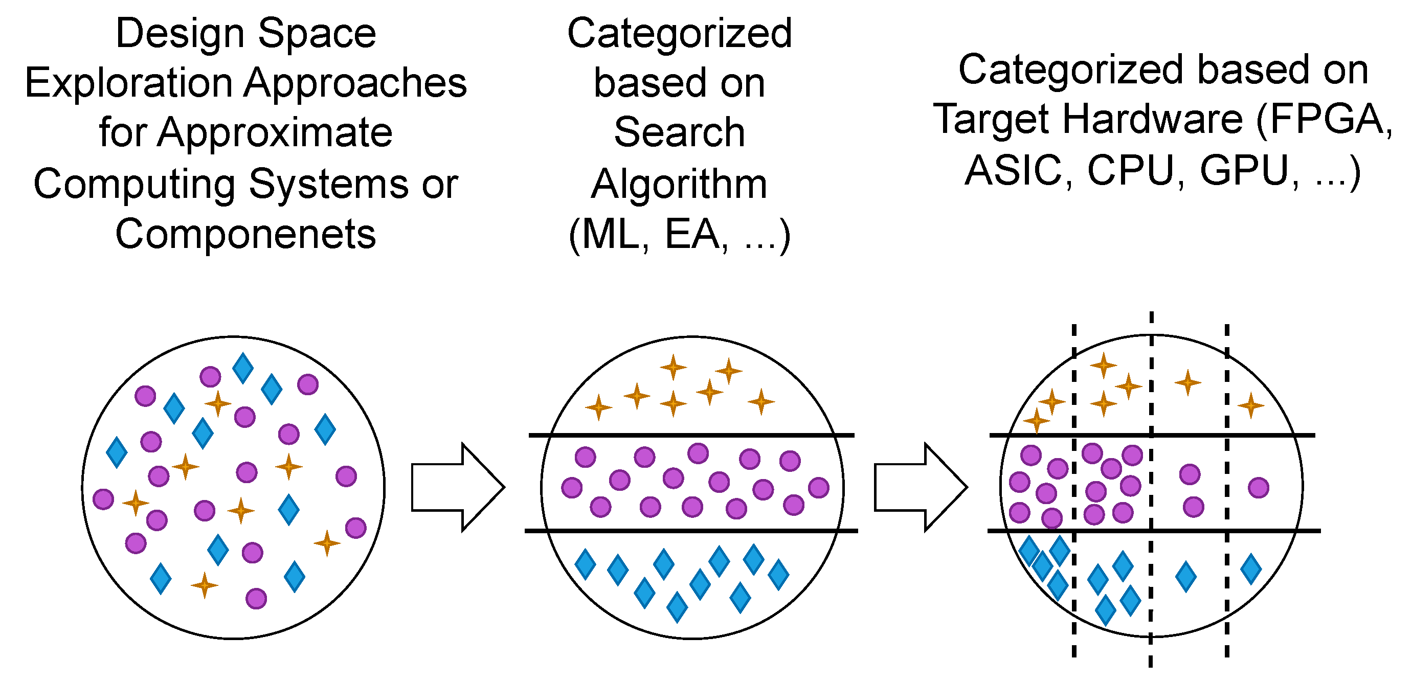

Table 1.
Precision metrics in Approximate Computing [36].
Table 1.
Precision metrics in Approximate Computing [36].
| Metric | Description | Application Domain |
|---|---|---|
| ER | Error Rate – Erroneous results per total results | General Computing |
| EP | Error Probability – Probability of error occurrence | |
| MED/MRED | Mean (Relative) Error Distance | |
| NMED/NMRED | Normalized Mean (Relative) Error Distance | |
| Max ED/RED | Maximum (Relative) Error Distance | |
| PED/PRED | Probability of (Relative) Error Distance > X | |
| MSE | Mean Squared Error | |
| RMSE | Root Mean Squared Error | |
| HD | Hamming Distance | |
| BER | Bit Error Ratio – Bit errors per total received bits | Digital Systems, Telecommunications |
| PER | Packet Error Ratio – Incorrect packets per total received packets | |
| PSNR | Peak Signal-to-Noise Ratio – Quality measurement between images | Image Processing, Video Processing, Computer Vision |
| SSIM | Structural Similarity – Quality measurement between images | |
| MPD | Mean Pixel Difference | |
| Classif. Accuracy | Correct classifications per total classifications | Pattern Recognition, Information Retrieval, Machine Learning |
| Precision | Relevant instances per total retrieved instances | |
| Recall | Relevant instances per total relevant instances |
Table 2.
Research works using ML-based search algorithms to perform the DSE.
| Year | Ref. | Target | Use Case | Benchmarks | Search |
| Hardware | Domains | Algorithm | |||
| 2018 | [52] | fpga | image processing | iris scanning | Reinforcement Learning (RL) |
| 2021 | [53] | fpga | image processing | kernel-based Gaussian blur filter | Multi-objective Bayesian Optimization (MBO) |
| 2019 | [12] | Accelerator (asic) | image processing | Sobel, and Gaussian blur filters (one with fixed coefficients, and one with a 3x3 kernel) | ML-based heuristic |
| 2023 | [54] | Accelerator (asic) | signal and image processing, and general arithmetic | Adder Tree, RGB2gray, Finite Impulse Response (FIR), and Gaussian blur filters | Artificial Intelligence (AI)-based heuristic: modified Monte Carlo Tree Search (MCTS) |
| 2021 | [55] | fpga, asic, General-purpose computing system | image processing | RGB2GRAY, Ternary sum. FIR, image sharpening, and Gaussian blur filters | ML |
| 2015 | [56] | General-purpose hardware (heterogeneous mobile, tablet, and server processors) | video encoder, financial analysis, image processing, search engine, digital signal processing, netlist place-and-route, image similarity search, and clustering algorithm | x264, Swaptions, Bodytrack, Swish++, Radar, Canneal, Ferret, and Streamcluster | RL |
| 2020 | [57] | General-purpose cpu and dnn accelerator | dnn for Image and Digit Classification | AlexNet, SimpleNet, LeNet, MobileNet, ResNet-20, 10-Layers, and VGG-11/16 | RL |
| 2023 | [38] | General-purpose cpu | ML, digital signal processing, and image processing | Matrix Multiplication, and FIR filter | RL |
Table 3.
Research works using ea as a search algorithm to perform the DSE.
| Year | Ref. | Target | Use Case | Benchmarks | Search |
| Hardware | Domains | Algorithm | |||
| 2021 | [58,59] | fpga | Image Processing | pixel-streaming pipeline | ga |
| 2023 | [60] | fpga-based approximate accelerator | High-Efficiency Video Coding (HEVC) | Multiplierless Multiple Constant Multiplier (MCM) | es algorithm, and Non-dominated Sorted Genetic Algorithm-II (NSGA-II) |
| 2022 | [61] | Accelerator (fpga and asic) | Image processing (JPEG compression) | Discrete Cosine Transform (DCT) | NSGA-II |
| 2014 | [62] | General-purpose cpu (implied) | scientific computing, 3D gaming, 3D image rendering, signal, and image processing | Fast Fourier Transform (FFT), SOR, MC, SMM, LU, Zxing, JMEint, Imagefill, and raytracer | ga |
| 2023 | [63] | gpu | image classification using cnn | MobileNetV2, and ResNet50V2 | Neural Architecture Search (NAS) algorithms: EvoApproxNAS (based on NSGA-II), and Google Model Search |
Table 4.
Research works using custom search algorithms to perform the DSE.
| Year | Ref. | Target | Use Case | Benchmarks | Search |
| Hardware | Domains | Algorithm | |||
| 2016 | [64] | asic, and fpga | HEVC | Sum of Absolute Differences (SAD) | Custom |
| 2020 | [65] | asic, and fpga | image classification using dnn | ResNet-18/34/38/74, MobileNetV2, and Transformer-base/WikiText-103 | Custom |
| 2016 | [66] | asic (implied) | handwriting recognition, general arithmetic, multimedia, signal, and image processing | Array Multiplier, Carry Lookahead Adder, Kogge Stone Adder, Multiple and Accumulate, SAD, Euclidean distance, DCT, FFT, and FIR. All used in a dnn vector accelerator | Heuristic |
| 2019 | [67] | asic (implied) | HEVC | SAD | Custom |
| 2021 | [68] | asic (implied) | image processing | Sobel, FIR, and Gaussian blur filters, a ReLu Neuron, Euclidean distance | Custom |
| 2017 | [69] | VLSI systems and High-Level Synthesis (HLS), aligning with asic design | image processing | average number calculator, inverse DCT calculator, Sobel, FIR, interpolation and decimation filters | Custom |
| 2020 | [70] | HLS tools for accelerator design | Image processing | Sobel and Sharpen filters | Tabu Search (TS) with potential integration of ga |
Table 5.
Research works using custom search algorithms to perform the DSE (continued.)
| Year | Ref. | Target | Use Case | Benchmarks | Search |
| Hardware | Domains | Algorithm | |||
| 2018 | [71] | hardware accelerator (asic implied) | ML, digital signal processing, and image processing | Matrix Multiplication, Sobel filter, and DCT | Custom |
| 2016 | [72] | ML accelerator (asic) | Image Processing, and NLP / Text Classification | Eye, and Face detection. Optical digit, Digit, Webpage, and Text classification | Gradient Descent (GD) |
| 2021 | [73,74] | asic (AI Accelerator) | image processing, NLP, and speech recognition | VGG16, ResNet50, InceptionV3, InceptionV4, MobileNetV1, SSD300, YoloV3, YoloV3-Tiny, BERT, a 2-layer LSTM, and a 4-layer bidirectional LSTM | Custom |
| 2016 | [75] | npu (asic) | financial analysis, robotics, 3D gaming, image compression, signal, and image processing | Blackscholes, FFT, Inversek2j, Jmeint, JPEG, Sobel filter | Custom |
| 2019 | [76] | Not specified (implied general-purpose) | image processing | Matrix Multiplication, and FIR filter | Custom |
| 2016 | [77] | gpu | For gpu: ML, signal processing (pattern recognition), image processing, medical imaging, scientific computing, and web mining. For cpu: scientific computing and optimization. | For gpu: Backprop, Fastwalsh, Gaussian, Heartwall, Matrixmul, Particle filter, Similarity score, S.reduce, S.srad2, and String match. For cpu: Bwaves, CactusADM, FMA3D, GemsFDTD, Soplex, and Swim. | Custom |
Table 6.
Research works that perform the DSE for approximate functions design space instead of a complete system.
Table 6.
Research works that perform the DSE for approximate functions design space instead of a complete system.
| Year | Ref. | Target | Use Case | Benchmarks | Search |
| Hardware | Domains | Algorithm | |||
| 2021 | [78] | fpga (also asic implied) | NA | apex2, b12, clip, duke2, and vg2 benchmarks from IWLS’93 Benchmark Set | NSGA-II |
| 2014 | [79] | fpga and asic (implied) | NA | Ripple Carry, Carry Lookahead, and Kogge Stone Adders. Wallace, and Dadda Multipliers. | Custom |
| 2021 | [80] | fpga and asic (designing fault-tolerant architectures) | safety-critical applications: Quadruple Approximate Modular Redundancy (QAMR) | generic combinational circuits | NSGA-II |
| 2021 | [81] | fpga and asic (implied) | NA | approximate adders, multipliers, divisor, barrel shifter, Sine, and Square | Heuristic |
| 2022 | [82] | fpga | NA | approximate adders, multipliers, decoders, and ALUs | NSGA-II |
Table 7.
AxC techniques in research works using ML-based search algorithms to perform the DSE.
| Year | Ref. | Target | Benchmarks | AxC Techniques | ||
| Hardware | Software | Architectural | Hardware | |||
| 2018 | [52] | fpga | iris scanning | reducing search window size and the region of interest in iris images, reducing the parameters of iris segmentation | NA | reducing the filter kernel size |
| 2021 | [53] | fpga | kernel-based Gaussian blur filter | approximation of the window size, mode, and stride length for convolution kernels | NA | approximate multipliers, and adders |
| 2019 | [12] | Accelerator (asic) | Sobel, and Gaussian blur filters (one with fixed coefficients, and one with a 3x3 kernel) | NA | NA | approximate adders and multipliers |
| 2023 | [54] | Accelerator (asic) | Adder Tree, RGB2gray, FIR, and Gaussian blur filters | NA | NA | approximate adders and multipliers |
| 2021 | [55] | fpga, asic, General-purpose computing system | RGB2GRAY, Ternary sum. FIR, image sharpening, and Gaussian blur filters | NA | NA | approximate adders and multipliers |
| 2015 | [56] | General-purpose hardware (heterogeneous mobile, tablet, and server processors) | x264, Swaptions, Bodytrack, Swish++, Radar, Canneal, Ferret, and Streamcluster | PowerDial (changes program inputs data structure), and Loop Perforation | NA | NA |
| 2020 | [57] | General-purpose cpu and dnn accelerator | AlexNet, SimpleNet, LeNet, MobileNet, ResNet-20, 10-Layers, and VGG-11/16 | dnn layer Quantization | NA | NA |
| 2023 | [38] | General-purpose cpu | Matrix Multiplication, and FIR filter | NA | NA | approximate adders and multipliers |
Table 8.
AxC techniques in research works using ea as a search algorithm to perform the DSE.
| Year | Ref. | Target | Benchmarks | AxC Techniques | ||
| Hardware | Software | Architectural | Hardware | |||
| 2021 | [58,59] | fpga | pixel-streaming pipeline | NA | NA | Sparse lut, Precision Scaling, Approximate Adders |
| 2023 | [60] | fpga-based approximate accelerator | Multiplierless MCM | NA | NA | approximate adders and multipliers |
| 2022 | [61] | Accelerator (fpga and asic) | DCT | NA | NA | approximate adders |
| 2014 | [62] | General-purpose cpu (implied) | FFT, SOR, MC, SMM, LU, Zxing, JMEint, Imagefill, and raytracer | program static instructions | NA | NA |
| 2023 | [63] | gpu | MobileNetV2, and ResNet50V2 | approximate 8xN bit multipliers emulated using lut, approximate depthwise convolution, and quantization-aware training | NA | NA |
Table 9.
AxC techniques in research works using custom search algorithms to perform the DSE.
| Year | Ref. | Target | Benchmarks | AxC Techniques | ||
| Hardware | Software | Architectural | Hardware | |||
| 2016 | [64] | asic, and fpga | SAD | NA | NA | approximate adders and logic blocks |
| 2020 | [65] | asic, and fpga | ResNet-18/34/38/74, MobileNetV2, and Transformer-base/WikiText-103 | Progressive Fractional Quantization (PFQ), Dynamic Fractional Quantization (DFQ) | NA | NA |
| 2016 | [66] | asic (implied) | Array Multiplier, Carry Lookahead Adder, Kogge Stone Adder, Multiple and Accumulate, SAD, Euclidean distance, DCT, FFT, and FIR. All used in a dnn vector accelerator | NA | NA | Logic isolation using latches or AND/OR gates at the inputs, MUXes at the output, and power gating |
| 2019 | [67] | asic (implied) | SAD | NA | NA | Approximate adders |
| 2021 | [68] | asic (implied) | Sobel, FIR, and Gaussian blur filters, a ReLu Neuron, Euclidean distance | NA | NA | Clock-gating, and Precision reduction of primary inputs at the RTL level |
| 2017 | [69] | VLSI systems and HLS, aligning with asic design | average number calculator, inverse DCT calculator, Sobel, FIR, interpolation and decimation filters | Source-Code Pruning Based on Profiling | Functional Unit Substitution (additions and multiplications) at the HLS level | Internal Signal Substitution, and Bit-Level Optimization at the RTL level |
| 2020 | [70] | HLS tools for accelerator design | Sobel and Sharpen filters | NA | NA | approximate adders and multipliers |
Table 10.
AxC techniques in research works using custom search algorithms to perform the DSE (continued.)
Table 10.
AxC techniques in research works using custom search algorithms to perform the DSE (continued.)
| Year | Ref. | Target | Benchmarks | AxC Techniques | ||
| Hardware | Software | Architectural | Hardware | |||
| 2018 | [71] | hardware accelerator (asic implied) | Matrix Multiplication, Sobel filter, and DCT | partial product perforation in approximate multipliers, and truncation in approximate adders/subtractors | NA | inexact compressor in approximate multipliers, approximate full adder, and VOS |
| 2016 | [72] | ML accelerator (asic) | Eye, and Face detection. Optical digit, Digit, Webpage, and Text classification | NA | NA | Clock Overgating |
| 2021 | [73,74] | asic (AI Accelerator) | VGG16, ResNet50, InceptionV3, InceptionV4, MobileNetV1, SSD300, YoloV3, YoloV3-Tiny, BERT, a 2-layer LSTM, and a 4-layer bidirectional LSTM | NA | precision reduction | approximated activation functions, pooling, normalization, and data shuffling |
| 2016 | [75] | npu (asic) | Blackscholes, FFT, Inversek2j, Jmeint, JPEG, Sobel filter | NA | Use of nn (npu accelerator) | NA |
| 2019 | [76] | Not specified (implied general-purpose) | Matrix Multiplication, and FIR filter | NA | NA | approximate adders and multipliers |
| 2016 | [77] | gpu | For gpu: Backprop, Fastwalsh, Gaussian, Heartwall, Matrixmul, Particle filter, Similarity score, S.reduce, S.srad2, and String match. For cpu: Bwaves, CactusADM, FMA3D, GemsFDTD, Soplex, and Swim. | NA | NA | Rollback-Free Value Prediction (RFVP) |
Table 11.
AxC techniques in research works that perform the DSE for approximate functions design space instead of a complete system.
Table 11.
AxC techniques in research works that perform the DSE for approximate functions design space instead of a complete system.
| Year | Ref. | Target | Benchmarks | AxC Techniques | ||
| Hardware | Software | Architectural | Hardware | |||
| 2021 | [78] | fpga (also asic implied) | apex2, b12, clip, duke2, and vg2 benchmarks from IWLS’93 Benchmark Set | NA | NA | Logic Falsification |
| 2014 | [79] | fpga and asic (implied) | Ripple Carry, Carry Lookahead, and Kogge Stone Adders. Wallace, and Dadda Multipliers. | NA | NA | Boolean network simplifications allowed by exdc |
| 2021 | [80] | fpga and asic (designing fault-tolerant architectures) | generic combinational circuits | NA | NA | Logic Falsification |
| 2021 | [81] | fpga and asic (implied) | approximate adders, multipliers, divisor, barrel shifter, Sine, and Square | NA | NA | Approximation based on Boolean Matrix Factorization (BMF) for truth tables |
| 2022 | [82] | fpga | approximate adders, multipliers, decoders, and ALUs | NA | NA | customized approximation of Boolean networks |
Table 12.
Evaluated metrics in research works using ML-based search algorithms to perform the DSE.
| Year | Ref. | Accu- racy | Error Metric(s) | Power or Energy | Time | Perfor- mance | Memory | Area | Pareto Front |
| 2018 | [52] | Industry level threshold for iris encoding | HD of any two images | Energy | Exe- cution time | NA | Memory utilization | Total Logic Utilization | Speedup and Average Error |
| 2021 | [53] | Appli- cation level Error | Mean Absolute Error (MAE) | NA | NA | NA | NA | lut count | lut count and Application level Error |
| 2019 | [12] | qor | SSIM | Energy | NA | NA | NA | Area | SSIM and Area. SSIM and Energy. |
| 2023 | [54] | Output Accuracy | MRED, and PSNR | NA | NA | NA | NA | Area | Area savings and Error |
| 2021 | [55] | Output Accuracy | MRED, and PSNR | Power | NA | NA | NA | Area | NA |
| 2015 | [56] | Appli- cation accuracy | Precision and Recall, PSNR, Swaption price, Track quality, Wire Length, Similarity, Quality of Clustering | Energy efficiency | NA | Speedup | NA | NA | Energy savings and Accuracy |
| 2020 | [57] | Relative dnn Accuracy, and Quantization level | State of Relative Accuracy, and State of Quantization | Energy | NA | Speedup | NA | NA | State of Relative Accuracy and State of Quantization |
| 2023 | [38] | Output Accuracy | MAE | Power | Comp- utation time | NA | NA | NA | NA |
Table 13.
Evaluated metrics in research works using ea as a search algorithm to perform the DSE.
| Year | Ref. | Accu- racy | Error Metric(s) | Power or Energy | Time | Perfor- mance | Memory | Area | Pareto Front |
| 2021 | [58,59] | Output Image Quality | Color differences in perceptually uniform color space (CIELAB ) | Power | NA | NA | NA | NA | Power consumption and maximum |
| 2023 | [60] | Output Quality, qor | PSNR | Power | NA | NA | NA | lut count | Power and PSNR. lut count and PSNR. |
| 2022 | [61] | Output Image Quality | Mean Structural SIMilarity (MSSIM) and Structural DISSIMilarity (DSSIM) | Power | NA | NA | NA | Area | Area and DSSIM (for asic). lut count and DSSIM (for fpga). Power and DSSIM (for both). |
| 2014 | [62] | qor | ER, Average Entry Difference, MPD, (Average) Normalized Difference | Energy | NA | NA | NA | NA | NA |
| 2023 | [63] | cnn Top-1 Accuracy | Clas- sifica- tion Accuracy (%) | Energy of Multiplication in Convolutional layers | cnn training and inference time overhead | NA | NA | NA | Energy and cnn Accuracy |
Table 14.
Evaluated metrics in research works using custom search algorithms to perform the DSE.
| Year | Ref. | Accu- racy | Error Metric(s) | Power or Energy | Time | Perfor- mance | Memory | Area | Pareto Front |
| 2016 | [64] | Output Quality | BER (%) | Power | NA | Perfor- mance (Bit Rate) | NA | Area | NA |
| 2020 | [65] | dnn Accuracy | Clas- sifica- tion Accuracy (%) | Training Energy | Training Latency | NA | NA | NA | NA |
| 2016 | [66] | dnn Clas- sifica- tion Accuracy | Clas- sifica- tion Accuracy | Energy savings | NA | NA | NA | NA | NA |
| 2019 | [67] | Output Accuracy, and Coding efficiency | MAE, and Bjontegaard delta PSNR (BD-PSNR) | Power dissipation savings | NA | NA | NA | Circuit Area savings | MAE and total Power. MAE and Circuit Area. Power dissipation and BD-PSNR. Area and BD-PSNR. |
| 2021 | [68] | Output Accuracy | MRED | Energy reduction | NA | Perfor- mance | NA | Area overhead | Power and Output Accuracy |
| 2017 | [69] | Comp- utation Accuracy | MAE | Power | NA | Perfor- mance | NA | Circuit Area | Circuit Area and MAE |
| 2020 | [70] | Output Accuracy | MED, and PSNR | Power-Delay-Product (PDP) | NA | NA | NA | Area | Area and MED. PDP and MED. |
Table 15.
Evaluated metrics in research works using custom search algorithms to perform the DSE (continued.)
Table 15.
Evaluated metrics in research works using custom search algorithms to perform the DSE (continued.)
| Year | Ref. | Accu- racy | Error Metric(s) | Power or Energy | Time | Perfor- mance | Memory | Area | Pareto Front |
| 2018 | [71] | Output Accuracy | MRED | Power | NA | NA | NA | NA | Power and Error |
| 2016 | [72] | Output Quality | Clas- sifica- tion Accuracy | Energy | NA | NA | NA | NA | NA |
| 2021 | [73,74] | dnn Accuracy | Clas- sifica- tion Accuracy (%) | NA | Infe- rence Latency | Infe- rence compute efficiency, and Training throughput | NA | NA | NA |
| 2016 | [75] | Output Quality | MRED, Miss Rate, Image Difference | Energy reduction | NA | Speedup | NA | NA | NA |
| 2019 | [76] | Output Accuracy | Norm- alized Weigh- ted Error | NA | NA | NA | NA | NA | NA |
| 2016 | [77] | Output quality | For gpu: MRED, Average Euclidean Distance, Image Difference, Total Mismatch Rate, and Normalized RMSE (also for cpu.) | Energy | Exe- cution time | Speedup | Memory Bandwidth | NA | Product of Energy dissipation, Execution time, and Error traded off with Predictor size |
Table 16.
Evaluated metrics in research works that perform the DSE for approximate functions design space instead of a complete system.
Table 16.
Evaluated metrics in research works that perform the DSE for approximate functions design space instead of a complete system.
| Year | Ref. | Accu- racy | Error Metric(s) | Power or Energy | Time | Perfor- mance | Memory | Area | Pareto Front |
| 2021 | [78] | Circuit Output Accuracy | BER | NA | NA | NA | NA | NA | Resour- ces (in terms of Cubes and Literals) and BER |
| 2014 | [79] | Circuit Output Accuracy | Error magnitude, Error frequency constraints | NA | NA | NA | NA | NA | Norm- alized gate count and Error frequency |
| 2021 | [80] | NA | NA | NA | Critical Path Delay | NA | NA | Circuit Area | Delay gain and Area gain |
| 2021 | [81] | Circuit Output Accuracy | Norm- alized HD, and MAE | Power | NA | NA | NA | Area | Power and MAE. Area utilization and MAE. |
| 2022 | [82] | Accu- racy Degradation observable at Primary Outputs (POs) | ER | NA | NA | NA | NA | lut count | ER and lut count |
Disclaimer/Publisher’s Note: The statements, opinions and data contained in all publications are solely those of the individual author(s) and contributor(s) and not of MDPI and/or the editor(s). MDPI and/or the editor(s) disclaim responsibility for any injury to people or property resulting from any ideas, methods, instructions or products referred to in the content. |
© 2024 by the authors. Licensee MDPI, Basel, Switzerland. This article is an open access article distributed under the terms and conditions of the Creative Commons Attribution (CC BY) license (http://creativecommons.org/licenses/by/4.0/).
Copyright: This open access article is published under a Creative Commons CC BY 4.0 license, which permit the free download, distribution, and reuse, provided that the author and preprint are cited in any reuse.


