Submitted:
30 September 2024
Posted:
03 October 2024
You are already at the latest version
Abstract
Predicting the remaining useful life (RUL) of mechanical bearings is crucial in the industry. 1 Estimating the RUL enables the assessment of health bearing, maintenance planning, and signifi- 2 cant cost reduction, thereby fostering industrial development. Existing models rely on traditional 3 feature engineering, with feature changes because operating conditions pose a major challenge to 4 the generalization of RUL prediction models. This study focuses on neural network-based feature 5 engineering and the downstream prediction of the RUL, eliminating the need for specific prior 6 knowledge and simplifying the development and maintenance of models. Initially, a convolutional 7 neural network (CNN) model is employed for feature engineering. Subsequently, a bidirectional 8 long short-term memory network (Bi-LSTM) model is used to capture the time-series degradation 9 characteristics of the engineered features and predict the RUL through regression. Finally, the study 10 examines the influence of operating conditions in the model and integrates domain adaptation to 11 minimize differences in feature distribution, thereby enhancing the model’s generalizability for the 12 RUL prediction.
Keywords:
bearing
; RUL
; CNN
; Bi-LSTM
; domain adaptation
1. Introduction
Bearing life prediction is a critical technology in the industrial sector, meant to identify bearing health and predict its lifespan early to facilitate planned maintenance and reduce economic losses. With the advancement of sensors and big data, bearing damage prediction technology has rapidly developed, encompassing condition-based maintenance (CBM) and prognostics and health management (PHM) [1]. Initially applied in the aviation sector, these techniques have gradually expanded to other industrial fields. Existing bearing prediction methods can be broadly categorized into two types: traditional machine learning methods that incorporate prior knowledge and deep learning methods primarily driven by data.
Traditional machine learning methods utilize numerical analysis to extract valuable features based on prior knowledge and then select appropriate models for fitting. For example, Loutas et al. proposed an -SVR model for monitoring rolling bearing conditions based on wavelet transformation to extract relevant features and Wiener entropy [2]. Qian et al. introduced an RQA-AR model for bearing degradation state extraction using Kalman filtering [3]. Jin et al. proposed an AR model based on extended Kalman filtering [4], while Li et al. presented a degradation-hidden Markov model [5]. Traditional model-based approaches rely on extensive prior knowledge to extract damage feature parameters (for example, kurtosis and time–frequency domain correlation indicators) from data to build corresponding models. However, with the increasing integration and complexity of modern systems, constructing such models has become increasingly challenging.
With the rise of the convolutional neural network (CNN), recurrent neural network (RNN), and long short-term memory (LSTM) network [6,7,8], researchers have gradually introduced deep networks for deep feature extraction, the joint analysis of previously extracted features, and remaining useful life (RUL) regression prediction [9,10,11,12,13,14], with prior knowledge serving only as an auxiliary for model training. As the data integration capability of deep networks improves, collaborative multi-view prediction has also undergone significant developments. For instance, Ren et al. proposed a deep neural network (DNN) model for multibearing collaborative prediction by introducing a new frequency-domain feature in addition to the traditional time- and frequency-domain features [15].
Although integrating prior knowledge with deep models has enhanced predictive performance, factors, such as data volume and operating conditions have constrained model generalization. Thus, researchers have introduced transfer learning to address these issues. For example, in the offline stages, semi-supervised training is conducted. It is then applied in the online stages for domain-adaptation models to predict the RUL [16], with the aim of improving model generalization. However, a lack of data makes model training challenging. To address this issue, He et al. proposed a semi-supervised generative adversarial network (GAN) method for predicting the RUL using fault and suspension histories to generate more data [17].
Researchers no longer consider prior knowledge a necessary condition for extracting data features, achieving significant breakthroughs in fields, such as image classification and object detection using CNN [18,19,20,21,22]. Consequently, deeper and broader models have been developed for bearing fault detection. For instance, Wen et al. proposed a CNN model based on LeNet-5 for fault diagnosis [23], which extracts features using a method that converts signals into 2D images, thereby eliminating the need for manual feature engineering. Models, such as the NB-CNN by Chen et al. [24] and DNCNN by Jia et al. [25] have demonstrated excellent performance in damage diagnosis by directly extracting features from raw signals using neural networks. This approach reduces the reliance on prior knowledge and enhances the robustness of the trained models. However, most of these efforts focused on bearing fault identification rather than RUL prediction.
Therefore, this paper proposes a deep-learning-based model for predicting bearing life. This model automatically extracts features from bearing data points and reveals the temporal relationships among these points. This paper presents a CNN-Bi-LSTM model framework, where a CNN extracts signal features in discrete time, a Bi-LSTM captures the temporal characteristics of these discrete-time features, and regression predicts the RUL based on the extracted spatiotemporal features. In addition, a domain-adaptation module was integrated into the proposed model to enhance its generalization and provide better robustness under different operating conditions. Section 2 introduces the methods used in this experiment, Section 3 presents the research results and discussion, and Section 4 concludes the paper.
2. Materials and Methods
2.1. Methods
2.1.1. CNN-Bi-LSTM Model
Building on the traditional CNN and LSTM, we propose a neural network model for predicting the RUL of bearings under one operating condition. The proposed framework focuses on modelling and analysing raw data from two perspectives: feature extraction and regression prediction, ultimately forecasting the RUL.
The framework of this method is illustrated in Figure 1. The data fragmentation module slices the raw data to expand the dataset. The CNN module extracts features from data points, effectively representing the data after dimension reduction. The Bi-LSTM module captures temporal features between data points and performs regression prediction using the Conv1D module.
2.1.2. Raw Data
The experiment utilized the PHM2012 challenge dataset (FEMTO-ST Bearing Dataset) [26] provided by the FEMTO-ST Institute. This dataset consists of bearing data collected under three operational conditions and sampled at a frequency of 25.6 kHz. Data was recorded every 10s, resulting in 2560 samples per recording. The specifications of the dataset are listed in Table 1.
The dataset had a sampling interval of 10 s between sample points, with 2560 samples constituting one sample point, representing the features of that point. The sequence of sample collection was used to determine the order of the time series. The RUL was 339s for the Bearing1_4 dataset; however, it was rounded to 340 s for prediction convenience. This adjustment introduced some errors but they were manageable. The sample sizes of the datasets are listed in Table 2.
2.1.3. Data Processing
This experiment did not rely on conventional methods for extracting information from the time and frequency domains to evaluate bearing conditions. Instead, the experiment described the vibration state of the bearings in a more intuitive manner by extracting data amplitudes. The results are shown in Figure 2, where labels a, b, c, and d represent the data amplitudes of Bearing1_1, Bearing1_2, Bearing2_2, and Bearing3_2, respectively.The complete amplitude chart is provided in Appendix A.
The amplitude plots of the data clearly reflect the vibration intensity, providing additional insights into the experimental results.
Due to the limited volume of the dataset, traditional data augmentation techniques may introduce unnecessary noise into the generated data. Therefore, we collected one sample point (each containing 256 vibration features) within 0.1 s at every 10-second interval, enabling us to segment the data accordingly. Within this extremely short time span, the vibration state of the bearing remains stable, allowing each of the resulting 10 segments to represent the vibration state at a specific point. This approach effectively expanded the dataset tenfold, alleviating the issue of insufficient data for comprehensive model training. Finally, we used the average of these 10 segments as the final representation of the data.
2.1.4. Localized Feature Extraction
A CNN was used to extract the localized features of the bearing vibration signals. A diagram of the CNN architecture is depicted in Figure 3.
In the CNN architecture, we employed three convolutional layers, each followed by an activation function, batch normalization, and max pooling to process the data. Vibration data were primarily collected from sensors in horizontal and vertical directions. In the first layer, we used (1, 8) convolutional kernels to capture more global information and structural features from the data. Additionally, to improve the generalization of the model, we increased the number of channels from 1 to 16, allowing for a more comprehensive exploration of data point information. Given the characteristics of the vibration data, we utilized a rectified linear unit (ReLU) as the activation function to transform the post-convolution data into a new representation. This approach assisted the model in extracting and representing various feature types. To prevent overfitting, gradient vanishing, or exploding. Additionally, to accelerate training while improving model generalization, we applied batch normalization to further process the data. Max pooling was used to reduce dimensionality and extract higher-level feature representations from the data, thereby enhancing computational efficiency, reducing model complexity, and increasing model translational invariance. A similar process was applied to the second and third layers. However, for these convolutional layers, we utilized 1x4 kernels to effectively explore local information and capture detailed features within the data.
After processing through the CNN layers, the model captures high-level feature representations of the time series, while reducing the dimensionality of the data. This reduction helps decrease the computational complexity of the bidirectional LSTM (Bi-LSTM) and improves the overall computational efficiency of the model.
2.1.5. Long Timing-Related Feature Extraction
To explore the temporal information between the data points we designed a two-layer Bi-LSTM architecture. The utilization of a two-layer Bi-LSTM enables hierarchical feature learning, addresses long-term dependencies between data points, and reduces the likelihood of gradient vanishing leading to improved performance. While the model effectively captures temporal information between data points, it can increase computational complexity and lead to overfitting. Therefore, within the two-layer Bi-LSTM model, we incorporated a dropout function to mitigate the risk of overfitting. The extracted features were then used for regression prediction. The architecture of the Bi-LSTM is depicted in Figure 4.
2.1.6. Regression Prediction
The features extracted by the Bi-LSTM did not exhibit strong linear relationships. Instead of using traditional fully connected layers for RUL prediction, we propose the use of one-dimensional (1D) convolutional prediction. 1D convolutional layers possess strong nonlinear extraction capabilities and are widely used in processing 1d sequence data, such as text classification, speech recognition, signal processing, and time-series analysis. The use of 1D convolution allows for the extraction of more local information among the features. Moreover, to reduce the model complexity, alleviate the computational burden, and mitigate the risk of overfitting, we utilized only one layer of 1D convolution for the regression prediction.
2.1.7. Domain-Adaptation Model Framework
Based on the experimental results described above, we observed significant differences in the vibration data from the bearings under various operating conditions, including the same operating conditions. To enhance the robustness of the previously proposed model and enable it to adapt to various vibration data scenarios, we incorporated domain adaptation through transfer learning, thereby making the entire model framework more resilient.
The model architecture used to incorporate domain adaptation into the base model is illustrated in Figure 5.
The domain-adaptation module consists of three linear layers. Before the features entered the domain-adaptation module for training, gradient reversal processing was applied. This approach helps the model to adapt the features from the source domain to match those of the target domain, while minimizing feature discrepancy. The functionalities of the other modules in the model remained consistent with those of the base model. The target-domain data used in the domain-adaptation module were not included in the RUL training process. Finally, we utilized the Jensen–Shannon (JS) divergence (Eq.1) to assess the effectiveness of the domain-adaptation module. A larger JS divergence indicates greater differences in the feature distribution between datasets, whereas a smaller JS divergence indicates smaller differences.
The method without domain adaptation module is shown as Algorithm 1, while the method with domain adaptation module is shown as Algorithm 2.
| Algorithm 1 Algorithm without Domain Adaptation Module |
|
| Algorithm 2 Algorithm with Domain Adaptation Module |
|
2.2. Materials
2.2.1. Motivation
Most of the traditional RUL prediction methods preprocess the data through feature engineering, extract the time-frequency domain features of the data according to relevant prior knowledge, and then predict the bearing RUL after model training. Different methods extract corresponding features according to different prior knowledge, which undoubtedly increases the cost of feature engineering. At the same time, because the time-frequency domain features extracted by different feature projects are different, the relevant features extracted may not be applicable to different models. Therefore, this paper abandons the method of extracting relevant time-frequency domain features based on prior knowledge, and directly extracts the deep features of data through neural network model. This method can reduce the cost of feature engineering without selecting time-frequency domain features according to relevant prior knowledge, so that the model can be better applied to different data sets and then applied in industry. The CNN model can extract the deep features of the image, and the image itself belongs to a data type. Therefore, this paper uses CNN model to mine the deep features of a single data point. At the same time, bearing data belongs to time sequence data, and time sequence information is hidden between points, and the Bi-LSTM model has certain advantages in extracting time sequence information. Therefore, this paper adopts the Bi-LSTM model to mine the time sequence information between data points. Different situations may occur in the running process of bearings, which may lead to large differences in data collected under different working conditions or even under the same working condition. This paper uses the domain adaptation method in transfer learning to solve this problem. Therefore, a domain adaptive model based on CNN-Bi-LSTM is proposed to predict bearing RUL.
2.2.2. Reproducibility
The algorithm of the proposed method is shown in Algorithm 3.
| Algorithm 3 The algorithm of the method proposed in this paper |
|
2.2.3. Description of Models Used
In the field of bearing RUL prediction, mean absolute error (MAE) and root mean square error (RMSE) are usually used as evaluation indexes, and the lower the value, the better the performance of the model. The formula of MAE is shown in (Eq.2), and the formula of RMSE is shown in (Eq.3).
Where n represents the number of samples, represents the actual RUL of the data point, and represents the RUL of the data point predicted by the model.
2.2.4. Evaluation Methods
MAE evaluates the average magnitude of the errors between the predicted and actual values, offering a direct measure of prediction accuracy. It is particularly useful for applications where each error is equally important, as it does not square the differences, ensuring that all deviations contribute proportionally to the overall error.
RMSE, on the other hand, penalizes larger errors more heavily due to the squaring of differences between predicted and actual values. This makes it sensitive to outliers, meaning it highlights models that produce large deviations from actual RUL values. Therefore, RMSE is often preferred when large errors are particularly undesirable, and reducing them is a priority.
Both metrics provide complementary perspectives: MAE gives a straightforward view of overall error, while RMSE emphasizes the significance of larger mistakes in the prediction.
In this paper, the results of MAE and RMSE obtained were compared with those of others, and the results of different models were compared through ablation experiments to determine the validity of the proposed method.
3. Results and Discussion
3.1. Experimental Results of CNN Data Point Feature Extraction
In this paper, according to the multi-layer feature extraction model proposed by [27], a three-layer CNN model was built to initially extract the deep features of data points to represent a single data point.The model was validated using data sets from the Bearing Data Center at Case Western Reserve University (CWRU)[28].Table 3 shows the relevant parameters selected using the grid search method, and the relevant hyperparameters finally determined by the model through the grid search method.The data set is shown in Table 5.All CWRU data are shown in Table 4. It can be seen from the table that there are four types of data under the four working conditions: normal, inner ring damage, outer ring damage and ball damage. We represent all damage data as 1 and normal data as 0. At the same time, the data collected on the corresponding bearing in each file is for a period of time, so we take 256 data as one data point to divide all the data into multiple sample points for model training.
As can be seen from Table 5, the accuracy of the model on the training set and the test set reaches 100%. To further test the performance of the model, we tested the data sets under conditions 2, 3 and 4 with the model, and recorded the experimental results in Table 5.As can be seen from the table, for data sets under different conditions, the prediction accuracy of the model for fault data reached 100%, and for normal data sets, it also had a high accuracy (due to the small amount of data of normal samples, the prediction accuracy of the model for normal samples under different conditions did not reach 100%). At the same time, it can be seen from Figure 6 that when the model is trained for about 140 rounds, the model becomes stable and the prediction accuracy of the training set and test set reaches 100%.Combined with Table 5 and Figure 6, it can be shown that the model can mine the deep features of a single data point.
To further verify the effectiveness of the model in extracting the deep features of data points, we used the FEMTO-ST bearing dataset to train the above model. The FEMTO-ST bearing data set is a life-cycle data set, and the data itself does not have fault labels, so we label the data according to the bearing fault point (FOT) proposed by [10]. At the same time, the amplitude of the data can better reflect the running state of the bearing, so we select the relevant FOT points according to the amplitude of the data. The amplitude of the data is shown in Figure 7. Data before the FOT point is a normal sample (assigned 0), while data after the FOT point is a fault sample (assigned 1). The FOT points constructed by the two methods are shown in Table 6, and the relevant experimental results are recorded in Table 7.
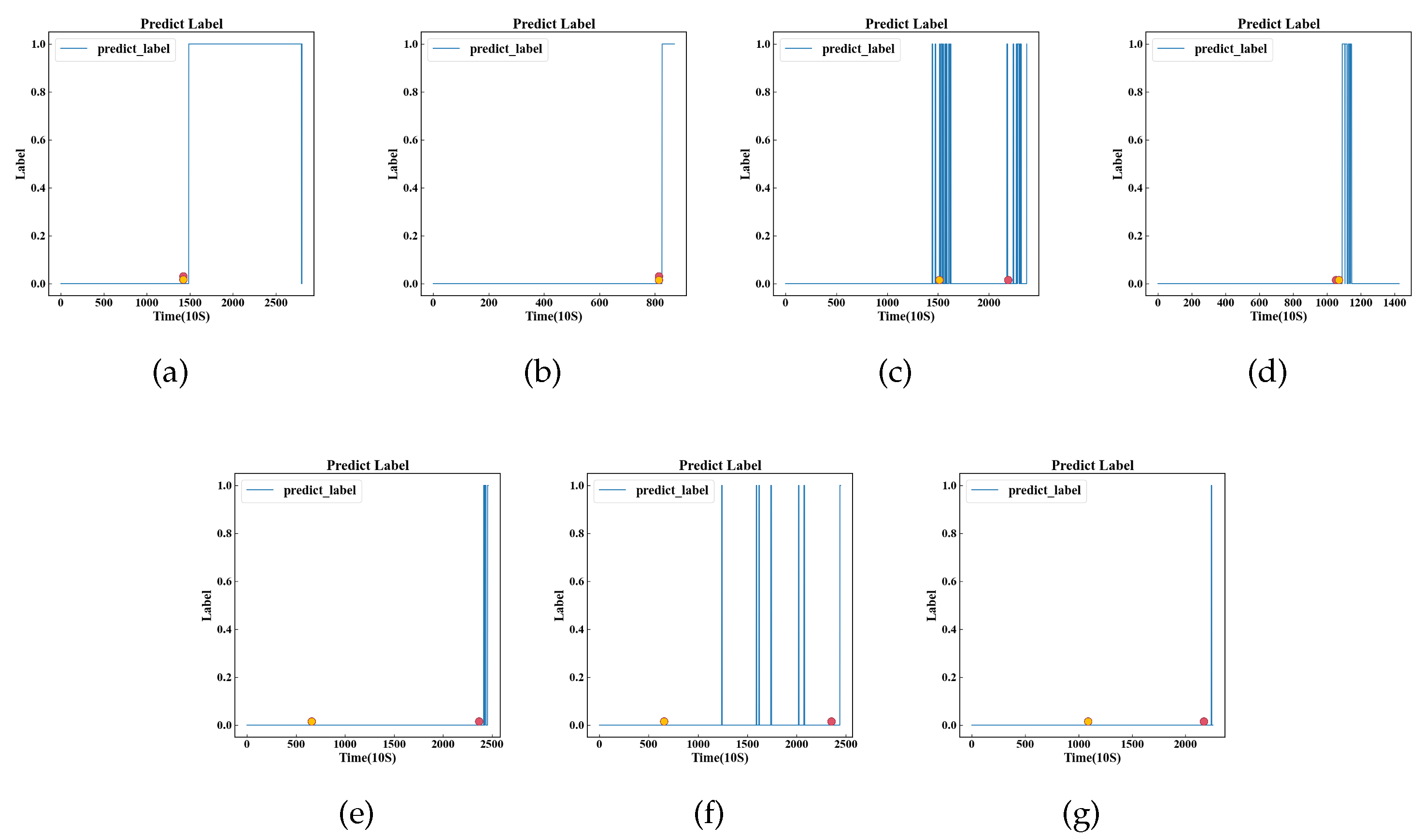
As can be seen from Table 7, the prediction performance of the model is significantly better according to the labels on the FOT points determined by the amplitude. In order to further determine the influence of FOT points, we plotted the predicted values of Bearing1_5, Bearing1_6 and Bearing1_7 models (three datasets with low accuracy) and the FOT points determined by the two methods in Figure 8. The full amplitude FOT point plot is documented in Appendices B.As can be seen from Figure 8, the FOT points determined based on the amplitude are closer to the predicted results of the model.
From the experimental results, the FOT points determined by the amplitude can better reflect the performance of the model. The original data used in this experiment is unprocessed, while the data used by [10]. is the time-frequency domain data obtained after pre-processing. The different feature distributions of the data lead to certain differences in the results. Through the above experiments, it can be determined that the built model can mine the deep features of a single data point, so that it can better represent the data point.
3.2. CNN-Bi-LSTM Model Experimental Results
In this experiment, trials were conducted using a model framework without domain adaptation. The method of using random search parameters was employed, ultimately determining the optimal parameters, which are listed in Table 8. As can be seen from Table 8, we used the Adam optimizer to adjust the learning rate, adjust the momentum, normalize the parameters, and prevent the model from overfitting.According to the characteristics of the label, we use the mean square error (MSE) as the loss function.To ensure a seamless connection between the CNN and LSTM layers, we used the batch size from the CNN as the sequence length for the LSTM network layer. To maintain the continuity of the time series, the batch size was sequentially rather than randomly partitioned.The entire experiment was conducted on a desktop computer equipped with a 12th Gen Intel(R) Core(TM) i5-12500 processor, running at 3.00 GHz, and utilizing the Windows 11 operating system.
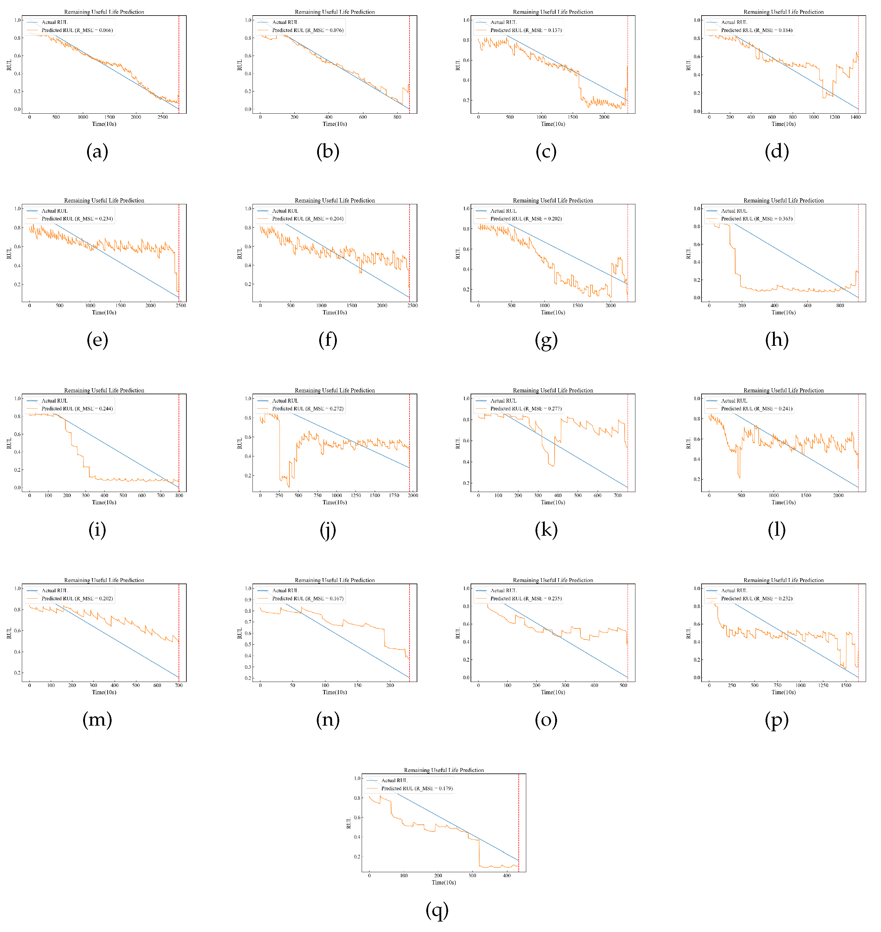
The experimental results are shown in Figure 9, where a–h represent the RUL for Bearing1_1, Bearing1_2, Bearing1_3, Bearing1_4, Bearing2_1, Bearing2_2, Bearing3_1, and Bearing3_2, respectively.Model predictions for all data sets in the three conditions are recorded in Appendices C.
In this experiment, the training set consisted of datasets Bearing1_1 and Bearing1_2 under operating condition one (OC1), while the remaining datasets served as the test set. Due to the varying lifespans of the datasets, direct lifespan values could not be used as training labels. Instead, we utilized a Health Indicator (HI) normalized between 0 and 1 for model training. From Fig.9, it can be observed that the model performed well with the training data set closely fitting the model. However, there were significant errors toward the end of the data due to limitations in the network structure. To ensure proper training, the dataset could not be fully partitioned, resulting in the exclusion of end-data points from the training. Consequently, the prediction performance for these end-data points was suboptimal, although the errors were controlled within an acceptable range. Furthermore, the performance of the test set for OC1 was notably better than those for OC2 and OC3. As shown in Fig.2, there were significant variations in the vibration data between different operating conditions and within similar conditions. The test set for OC1 exhibited satisfactory results, whereas for OC2, the model predicted stable labels during certain periods, indicating consistent degradation trends and minimal vibration fluctuations. Similarly, this pattern was observed for OC3. Overall, the test set predictions under the three operating conditions were satisfactory. The performance of the end-data points was suboptimal, similar to that of the training set, although within an acceptable range.
Table 9 presents the evaluation metrics used to compare our model with a published I-DCNN [29] model and MCNN [30] model. It can be observed from the table that our method achieved better results for most of the tested samples.
Time series features play an important role in RUL prediction. Therefore, we use different temporal basic models (such as BI-LSTM, LSTM, RNN, Bi-RNN, GRU, BI-GRU, etc.) to mine temporal features between data for RUL prediction. We only replace the network layer in the model that extracts the temporal features between data, and keep other parameters unchanged to carry out relevant experiments. The experimental results are recorded in Table 10.At the same time, all data sets under the three working conditions obtained by the model are recorded in Appendix A.
As can be seen from Table 10, the data set with the OC1 has the best prediction effect on the Bi-LSTM model, and its NRMSE is 0.1576. At the same time, most of the data sets show good performance in the BI-LSTM model, so we finally use the Bi-LSTM neural network model to mine the timing features between the data.
In addition, we observed a significant increase in the test set metrics for OC2 and OC3, indicating a decrease in predictive performance. This highlights the impact of operating conditions on the generalizability of the model. Beyond the training datasets (Bearing1_1 and Bearing1_2), we selected two samples from the test sets for each OC (Bearing1_3, Bearing1_4, Bearing2_1, Bearing2_2, Bearing3_1, and Bearing3_2) and examined the feature distribution using t-distributed stochastic neighbour embedding (t-SNE) downscaling. The results are displayed in Figure 10.
We can observe from the feature distribution plots that the feature distribution of the test set closely aligns with that of the training set. However, certain datasets show a high concentration of points, suggesting that the bearings were in a stable state during periods with similar vibration data. Consequently, the predictions during these periods yielded similar results, reflecting a stable operational state of bearings. Meanwhile, it can be seen from the figure that some feature regions of Bearing1_1 and Bearing1_2 are similar, but their RUL values are completely different. As a result, the model cannot accurately predict the RUL value on the test set, which reduces the performance of the model.To further quantify the results, we computed the JS divergence to compare the distribution similarity of the different datasets. The results are summarized in Table 11.
As can be seen from Table 11, the JS divergence between Bearing1_3 and Bearing1_2 is small and their feature region is similar; the JS divergence between Bearing1_3 and Bearing1_2 is large, and their feature region is similar is low and their prediction performance is good. However, the JS divergence between Bearing2_1 and the two training sets is not large or small, and the prediction result is sub-optimal. At the same time, the similarity of feature regions between Bearing1_1 and Bearing1_2 is high. Figure 10 further supports the effectiveness of the model in predicting the features of the data set. In addition, Table 11 confirms significant differences between the source and target domains, which lead to suboptimal experimental results.
To enhance the performance of the base model, reduce the disparities between the source- and target-domain feature distributions, and achieve more accurate predictions, we employed domain-adaptation methods to refine the model and improve its predictive effectiveness.
3.3. Domain-Adaptation Model Experimental Results
In this experiment, we implemented an adversarial domain-adaptation method based on the aforementioned base model, as depicted in Figure 5. From the experimental results mentioned earlier, We found that the regression layer was the main factor affecting the prediction result. Therefore, we kept the parameters of the CNN and LSTM layers unchanged while resetting the parameters of the regression prediction network layers for retraining. The basic experimental information is summarized in Table 12.
The evaluation metrics after domain adaptation are listed on Table 13. From the table, it can be seen that the indicators for Bearing1_1, Bearing2_1, Bearing3_1 and Bearing3_2 noticeably decreased, while those for Bearing2_2 did not show significant changes. Overall, the model was proven effective in enhancing predictive performance.
Therefore, it can be demonstrated that domain-adaptation techniques can minimize the disparities in feature distributions and improve model performance. Additionally, when a bearing is in a stable state, the collected vibration data is similar, leading to similar RUL values predicted by the model.
4. Conclusions
This paper proposed a neural-network-based method for predicting the RUL. This method leveraged a CNN to extract relevant features from data points and utilized a Bi-LSTM network to capture temporal relationships among the data, thereby replacing traditional feature engineering based on prior knowledge. Domain-adaptation techniques were employed to address significant data differences across multiple operating conditions. Experimental validation confirmed the effectiveness, correctness, and practicality of the proposed approach. The results demonstrated that this method can accurately predict the RUL and is suitable for industrial applications.The motivation of this paper is recorded in Appendices E, the reproducibility algorithm, relevant codes, selected data sets, etc. of the experiment are recorded in Appendices F, and the evaluation methods and evaluation indicators are recorded in Appendices G.
Despite achieving favourable results, the proposed method has several limitations:
- It failed to consider the actual scenario where bearing degradation begins after a period of operation, requiring RUL calculations to start from the onset of degradation.
- Even with data augmentation through data slicing, the dataset remains small, potentially limiting the ability of the model to fully explore intricate data features.
- Because of the characteristics of the network structure, the use of tail-end data is neglected, resulting in certain errors at the end of the dataset.
Future work will focus on identifying the point of initial bearing degradation (FOT) to uncover data degradation information more accurately. This involves the use of generative networks to create a significant amount of data within acceptable noise ranges to address data scarcity. Additionally, optimizing the network structure to effectively utilize tail-end data will be explored in future research.
Author Contributions
Conceptualization, F.L. and Y.C.; methodology, F.L. and Y.C..; software, F.L.; validation, F.L.; formal analysis, Y.C.; investigation, Z.D.; resources, L.J.; data curation, C.S.; writing—original draft preparation, F.L.; writing—review and editing, Y.C. and F.L.; visualization, F.L.; supervision, C.Z.; project administration, C.Z.; All authors have read and agreed to the published version of the manuscript.
Funding
This research was funded by NAME OF [the National Natural Science Foundation of China] grant number [12304513 and 62172242]; and [Ningbo Natural Science Foundation] grant number [2022J138].
Data Availability Statement
The CRWU dataset and the PHM2012 Challenger dataset are used in this article.(Two versions are available, compressed and uncompressed.) Related data sets to Google cloud disk, link is as follows: https://drive.google.com/drive/folders/1bXvElCVCr0smjgKW4a0feG5L8W9U08sq?usp=drivel.Meanwhile, we have uploaded the experimental code to GitHub. The link is: https://github.com/FeiFanLi-arch/phm2012_domain_cnn_bi_lstm.git. Detailed information is listed in the README file.
Conflicts of Interest
The authors declare no conflicts of interest.
Abbreviations
The following abbreviations are used in this manuscript:
| MDPI | Multidisciplinary Digital Publishing Institute |
| DOAJ | Directory of open access journals |
| TLA | Three letter acronym |
| LD | Linear dichroism |
Appendix A. Complete amplitude plots under three working conditions
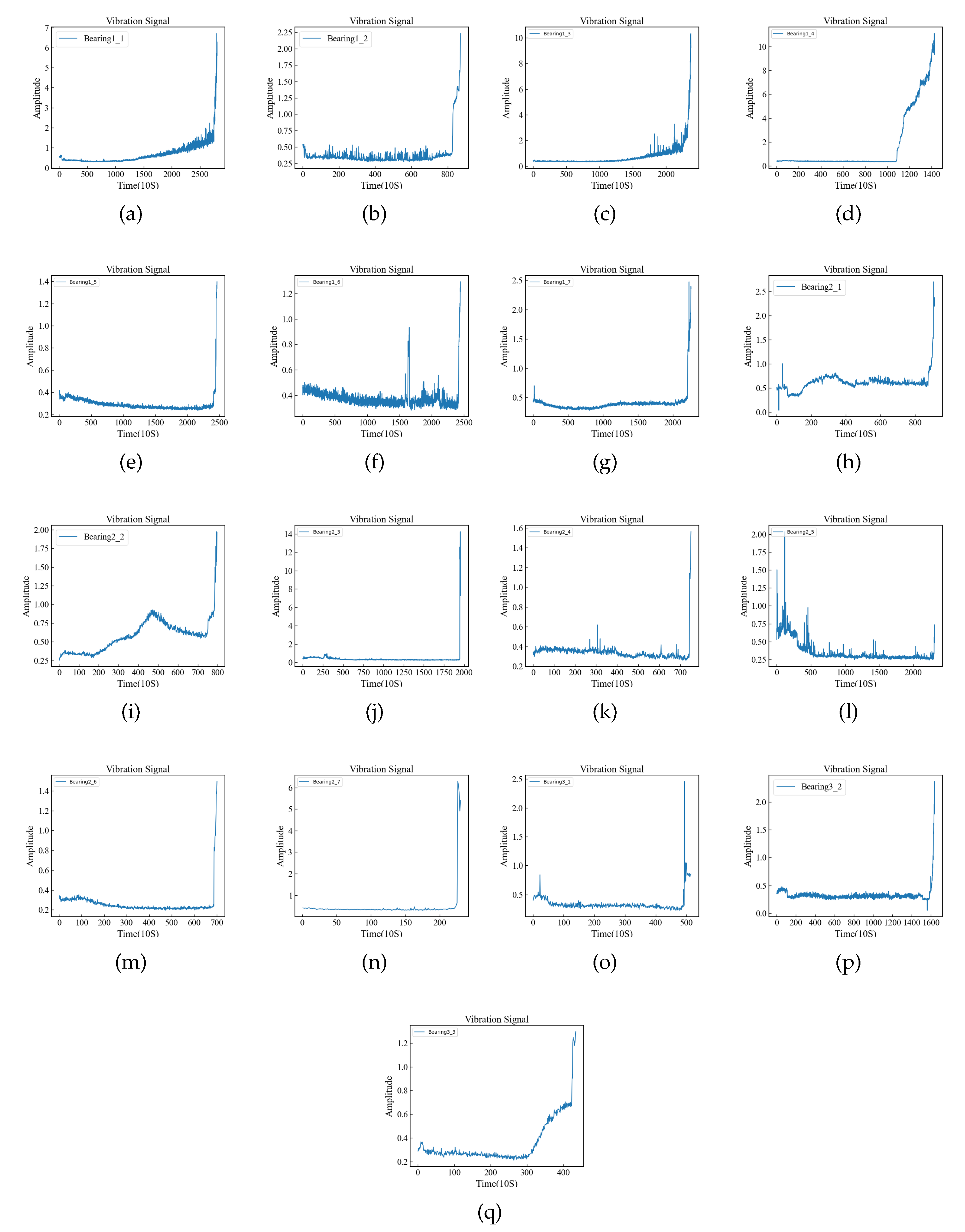
The amplitude diagram of all data sets under the three working conditions is shown in Figure A1, from which we can clearly see the running state of the bearing.
Figure A1.
The amplitude bearing data provides an in-depth understanding of the vibration magnitude and intensity experienced by bearings, serving as auxiliary conditions for RUL.(a-q expression Bearing1_1, Bearing1_2, Bearing1_3, Bearing1_4, Bearing1_5, Bearing1_6, Bearing1_7, Bearing2_1, Bearing2_2, Bearing2_3, Bearing2_4, Bearing2_5, Bearing2_6, Bearing2_7, Bearing3_1, Bearing3_2, Bearing3_3 amplitudes.)
Appendix B. Amplitude FOT point plot below the working condition
The FOT points and model prediction results obtained by two methods for all data sets are recorded in Figure A2.
Figure A2.
The model predicted values, where the red dots represent FOT points based on amplitude and the yellow dots represent FOT points based on [10].(a-g expression Bearing1_1, Bearing1_2, Bearing1_3, Bearing1_4, Bearing1_5, Bearing1_6, Bearing1_7 amplitudes and fots.)
Figure A2.
The model predicted values, where the red dots represent FOT points based on amplitude and the yellow dots represent FOT points based on [10].(a-g expression Bearing1_1, Bearing1_2, Bearing1_3, Bearing1_4, Bearing1_5, Bearing1_6, Bearing1_7 amplitudes and fots.)
Appendix C. Model prediction results of all data sets under three operating conditions
All the predicted results of the model are shown in Figure A3.
Figure A3.
For RUL prediction under various conditions, Bearing1_1 and Bearing1_2 under OC1 are used as training sets. The test set is as follows: Bearing1_3 and Bearing1_4 under OC1, Bearing2_1 and Bearing2_2 under OC2, and Bearing3_1 and Bearing3_2 under OC3 (corresponding to a-h in the figure). The yellow line indicates the predicted RUL, the blue line indicates the actual RUL, and the red line indicates the end of life.(a-q expression Bearing1_1, Bearing1_2, Bearing1_3, Bearing1_4, Bearing1_5, Bearing1_6, Bearing1_7, Bearing2_1, Bearing2_2, Bearing2_3, Bearing2_4, Bearing2_5, Bearing2_6, Bearing2_7, Bearing3_1, Bearing3_2, Bearing3_3 RUL.)
Appendix D. All relevant indicators obtained under all models are recorded in Table A1.
It can be seen from Table A1 that under the Bi-LSTM time series model, the relevant indicators of most data sets are optimal.

Table A1.
Comparative analysis of the performance of various time series models.
| Bi-LSTM | LSTM | RNN | Bi-RNN | GRU | Bi-GRU | |||||||
| Bearing | MAE | RMSE | MAE | RMSE | MAE | RMSE | MAE | RMSE | MAE | RMSE | MAE | RMSE |
| 1_1 | 0.0511 | 0.0662 | 0.2501 | 0.2888 | 0.2533 | 0.2943 | 0.2761 | 0.3307 | 0.2734 | 0.3124 | 0.0725 | 0.0918 |
| 1_2 | 0.0492 | 0.0759 | 0.2503 | 0.2890 | 0.2535 | 0.2946 | 0.2763 | 0.3309 | 0.1763 | 0.2400 | 0.0511 | 0.0697 |
| 1_3 | 0.1112 | 0.1370 | 0.2143 | 0.2539 | 0.2302 | 0.2780 | 0.2828 | 0.3459 | 0.2571 | 0.3174 | 0.1139 | 0.1447 |
| 1_4 | 0.1325 | 0.1840 | 0.2445 | 0.2825 | 0.2490 | 0.2901 | 0.2747 | 0.3306 | 0.2591 | 0.3058 | 0.1569 | 0.2171 |
| 1_5 | 0.1921 | 0.2341 | 0.2360 | 0.2733 | 0.2427 | 0.2845 | 0.2735 | 0.3316 | 0.2907 | 0.3490 | 0.2227 | 0.2796 |
| 1_6 | 0.1712 | 0.2035 | 0.2371 | 0.2744 | 0.2434 | 0.2851 | 0.2736 | 0.3313 | 0.3482 | 0.4121 | 0.1769 | 0.2395 |
| 1_7 | 0.1790 | 0.2024 | 0.2099 | 0.2524 | 0.2307 | 0.2816 | 0.2949 | 0.3570 | 0.3016 | 0.3625 | 0.0980 | 0.1264 |
| 2_1 | 0.3007 | 0.3634 | 0.2503 | 0.2890 | 0.2535 | 0.2945 | 0.2762 | 0.3309 | 0.3360 | 0.3789 | 0.1565 | 0.1890 |
| 2_3 | 0.1972 | 0.2722 | 0.2092 | 0.2532 | 0.2326 | 0.2847 | 0.3030 | 0.3632 | 0.3053 | 0.3662 | 0.1845 | 0.2449 |
| 2_4 | 0.2184 | 0.2769 | 0.2192 | 0.2574 | 0.2322 | 0.2779 | 0.2779 | 0.3404 | 0.2515 | 0.2949 | 0.2509 | 0.3160 |
| 2_5 | 0.1995 | 0.2407 | 0.2251 | 0.2625 | 0.2354 | 0.2792 | 0.2747 | 0.3356 | 0.3124 | 0.3717 | 0.2164 | 0.2707 |
| 2_6 | 0.1704 | 0.2016 | 0.2193 | 0.2575 | 0.2322 | 0.2779 | 0.2779 | 0.3403 | 0.2587 | 0.3150 | 0.2275 | 0.2689 |
| 2_7 | 0.1427 | 0.1667 | 0.2140 | 0.2542 | 0.2307 | 0.2793 | 0.2847 | 0.3484 | 0.2734 | 0.3350 | 0.1605 | 0.1927 |
| 3_1 | 0.1880 | 0.2353 | 0.2505 | 0.2893 | 0.2537 | 0.2948 | 0.2765 | 0.3312 | 0.3165 | 0.3657 | 0.1829 | 0.2442 |
| 3_2 | 0.1955 | 0.2316 | 0.2502 | 0.2889 | 0.2534 | 0.2944 | 0.2761 | 0.3308 | 0.3224 | 0.3840 | 0.2051 | 0.2488 |
| 3_3 | 0.1550 | 0.1786 | 0.2189 | 0.2573 | 0.2320 | 0.2780 | 0.2786 | 0.3411 | 0.3641 | 0.3998 | 0.0982 | 0.1182 |
References
- Zhao, Z.; Liang, B.; Wang, X.; Lu, W. Remaining useful life prediction of aircraft engine based on degradation pattern learning. Reliability Engineering & System Safety 2017, 164, 74–83. [Google Scholar]
- Loutas, T.H.; Roulias, D.; Georgoulas, G. Remaining useful life estimation in rolling bearings utilizing data-driven probabilistic E-support vectors regression. IEEE Transactions on Reliability 2013, 62, 821–832. [Google Scholar] [CrossRef]
- Qian, Y.; Yan, R.; Hu, S. Bearing degradation evaluation using recurrence quantification analysis and Kalman filter. IEEE Transactions on Instrumentation and Measurement 2014, 63, 2599–2610. [Google Scholar] [CrossRef]
- Jin, X.; Sun, Y.; Que, Z.; Wang, Y.; Chow, T.W. Anomaly detection and fault prognosis for bearings. IEEE Transactions on Instrumentation and Measurement 2016, 65, 2046–2054. [Google Scholar] [CrossRef]
- Li, J.; Zhang, X.; Zhou, X.; Lu, L. Reliability assessment of wind turbine bearing based on the degradation-Hidden-Markov model. Renewable energy 2019, 132, 1076–1087. [Google Scholar] [CrossRef]
- LeCun, Y.; Bottou, L.; Bengio, Y.; Haffner, P. Gradient-based learning applied to document recognition. Proceedings of the IEEE 1998, 86, 2278–2324. [Google Scholar] [CrossRef]
- Elman, J.L. Finding structure in time. Cognitive science 1990, 14, 179–211. [Google Scholar] [CrossRef]
- Hochreiter, S.; Schmidhuber, J. Long short-term memory. Neural computation 1997, 9, 1735–1780. [Google Scholar] [CrossRef]
- Li, X.; Zhang, W.; Ding, Q. Deep learning-based remaining useful life estimation of bearings using multi-scale feature extraction. Reliability engineering & system safety 2019, 182, 208–218. [Google Scholar]
- Zhu, J.; Chen, N.; Shen, C. A new data-driven transferable remaining useful life prediction approach for bearing under different working conditions. Mechanical Systems and Signal Processing 2020, 139, 106602. [Google Scholar] [CrossRef]
- Cheng, C.; Ma, G.; Zhang, Y.; Sun, M.; Teng, F.; Ding, H.; Yuan, Y. A deep learning-based remaining useful life prediction approach for bearings. IEEE/ASME transactions on mechatronics 2020, 25, 1243–1254. [Google Scholar] [CrossRef]
- Cao, Y.; Ding, Y.; Jia, M.; Tian, R. A novel temporal convolutional network with residual self-attention mechanism for remaining useful life prediction of rolling bearings. Reliability Engineering & System Safety 2021, 215, 107813. [Google Scholar]
- Wang, B.; Lei, Y.; Yan, T.; Li, N.; Guo, L. Recurrent convolutional neural network: A new framework for remaining useful life prediction of machinery. Neurocomputing 2020, 379, 117–129. [Google Scholar] [CrossRef]
- Chen, Y.; Peng, G.; Zhu, Z.; Li, S. A novel deep learning method based on attention mechanism for bearing remaining useful life prediction. Applied Soft Computing 2020, 86, 105919. [Google Scholar] [CrossRef]
- Ren, L.; Cui, J.; Sun, Y.; Cheng, X. Multi-bearing remaining useful life collaborative prediction: A deep learning approach. Journal of Manufacturing Systems 2017, 43, 248–256. [Google Scholar] [CrossRef]
- Zeng, F.; Li, Y.; Jiang, Y.; Song, G. An online transfer learning-based remaining useful life prediction method of ball bearings. Measurement 2021, 176, 109201. [Google Scholar] [CrossRef]
- He, R.; Tian, Z.; Zuo, M.J. A semi-supervised GAN method for RUL prediction using failure and suspension histories. Mechanical Systems and Signal Processing 2022, 168, 108657. [Google Scholar] [CrossRef]
- Simonyan, K.; Zisserman, A. Very deep convolutional networks for large-scale image recognition. arXiv preprint arXiv:1409.1556, arXiv:1409.1556 2014.
- Szegedy, C.; Liu, W.; Jia, Y.; Sermanet, P.; Reed, S.; Anguelov, D.; Erhan, D.; Vanhoucke, V.; Rabinovich, A. Going deeper with convolutions. Proceedings of the IEEE conference on computer vision and pattern recognition, 2015, pp. 1–9. [CrossRef]
- He, K.; Zhang, X.; Ren, S.; Sun, J. Deep residual learning for image recognition. Proceedings of the IEEE conference on computer vision and pattern recognition, 2016, pp. 770–778. [CrossRef]
- Ren, S.; He, K.; Girshick, R.; Sun, J. Faster r-cnn: Towards real-time object detection with region proposal networks. Advances in neural information processing systems 2015, 28. [Google Scholar] [CrossRef]
- Kong, T.; Yao, A.; Chen, Y.; Sun, F. Hypernet: Towards accurate region proposal generation and joint object detection. Proceedings of the IEEE conference on computer vision and pattern recognition, 2016, pp. 845–853. [CrossRef]
- Wen, L.; Li, X.; Gao, L.; Zhang, Y. A new convolutional neural network-based data-driven fault diagnosis method. IEEE Transactions on Industrial Electronics 2017, 65, 5990–5998. [Google Scholar] [CrossRef]
- Chen, F.C.; Jahanshahi, M.R. NB-CNN: Deep learning-based crack detection using convolutional neural network and Naïve Bayes data fusion. IEEE Transactions on Industrial Electronics 2017, 65, 4392–4400. [Google Scholar] [CrossRef]
- Jia, F.; Lei, Y.; Lu, N.; Xing, S. Deep normalized convolutional neural network for imbalanced fault classification of machinery and its understanding via visualization. Mechanical Systems and Signal Processing 2018, 110, 349–367. [Google Scholar] [CrossRef]
- Nectoux, P.; Gouriveau, R.; Medjaher, K.; Ramasso, E.; Chebel-Morello, B.; Zerhouni, N.; Varnier, C. PRONOSTIA: An experimental platform for bearings accelerated degradation tests. IEEE International Conference on Prognostics and Health Management, PHM’12. IEEE Catalog Number: CPF12PHM-CDR, 2012, pp. 1–8.
- Li, X.; Zhang, W.; Ding, Q. Deep learning-based remaining useful life estimation of bearings using multi-scale feature extraction. Reliability Engineering & System Safety 2019, 182, 208–218. [Google Scholar] [CrossRef]
- Smith, W.A.; Randall, R.B. Rolling element bearing diagnostics using the Case Western Reserve University data: A benchmark study. Mechanical systems and signal processing 2015, 64, 100–131. [Google Scholar] [CrossRef]
- Guo, Y.; Zhang, H.; Xia, Z.; Dong, C.; Zhang, Z.; Zhou, Y.; Sun, H. An improved deep convolution neural network for predicting the remaining useful life of rolling bearings. Journal of Intelligent & Fuzzy Systems 2021, 40, 5743–5751. [Google Scholar]
- Zhu, J.; Chen, N.; Peng, W. Estimation of bearing remaining useful life based on multiscale convolutional neural network. IEEE Transactions on Industrial Electronics 2018, 66, 3208–3216. [Google Scholar] [CrossRef]
Figure 1.
The proposed experimental method is illustrated through a block diagram, showcasing the sequential steps and components involved in the process.
Figure 1.
The proposed experimental method is illustrated through a block diagram, showcasing the sequential steps and components involved in the process.
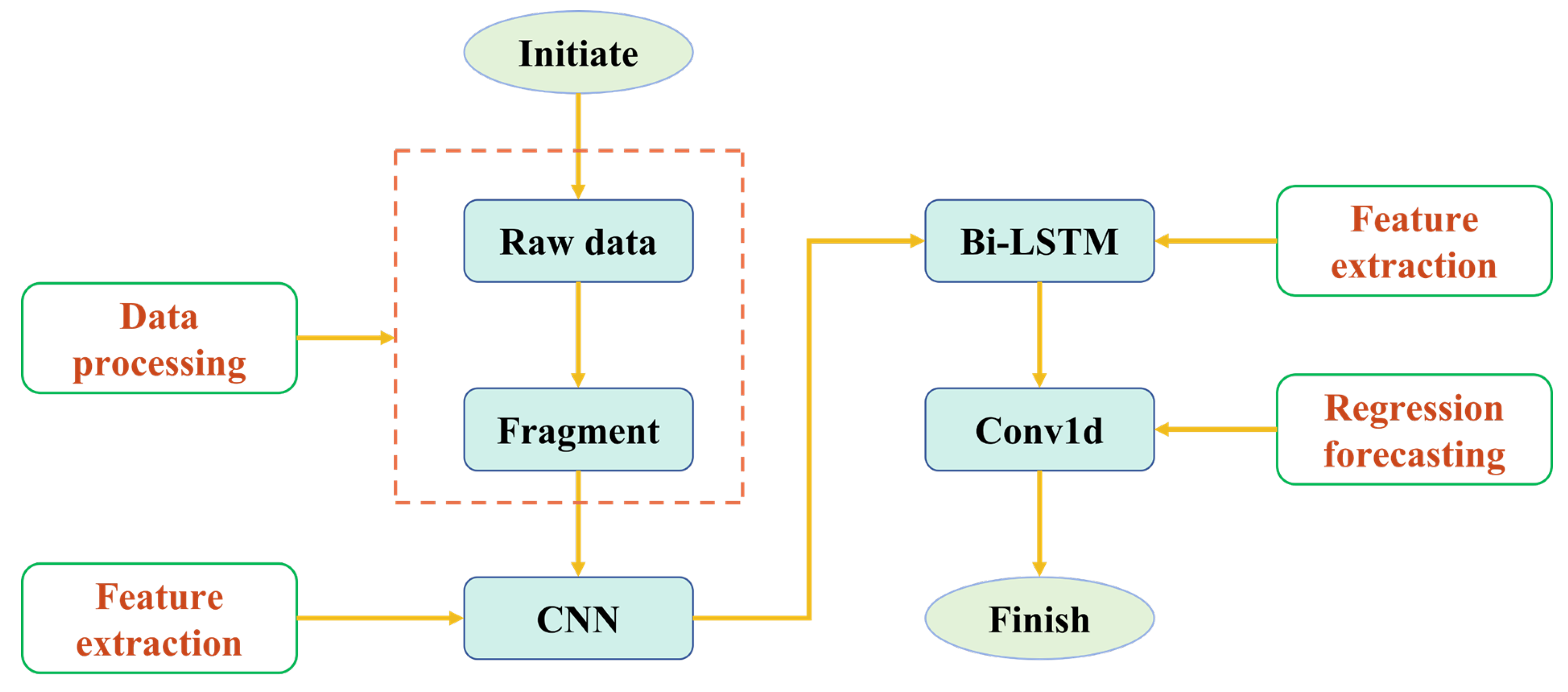
Figure 2.
The amplitude bearing data provides an in-depth understanding of the vibration magnitude and intensity experienced by bearings, serving as auxiliary conditions for RUL.(a-d indicates Bearing1_1 amplitude, Bearing1_2 amplitude, Bearing2_2 amplitude and Bearing3_2 amplitude.)
Figure 2.
The amplitude bearing data provides an in-depth understanding of the vibration magnitude and intensity experienced by bearings, serving as auxiliary conditions for RUL.(a-d indicates Bearing1_1 amplitude, Bearing1_2 amplitude, Bearing2_2 amplitude and Bearing3_2 amplitude.)

Figure 3.
The CNN structure diagram intuitively illustrates the changes in data dimensions within the network architecture.
Figure 3.
The CNN structure diagram intuitively illustrates the changes in data dimensions within the network architecture.
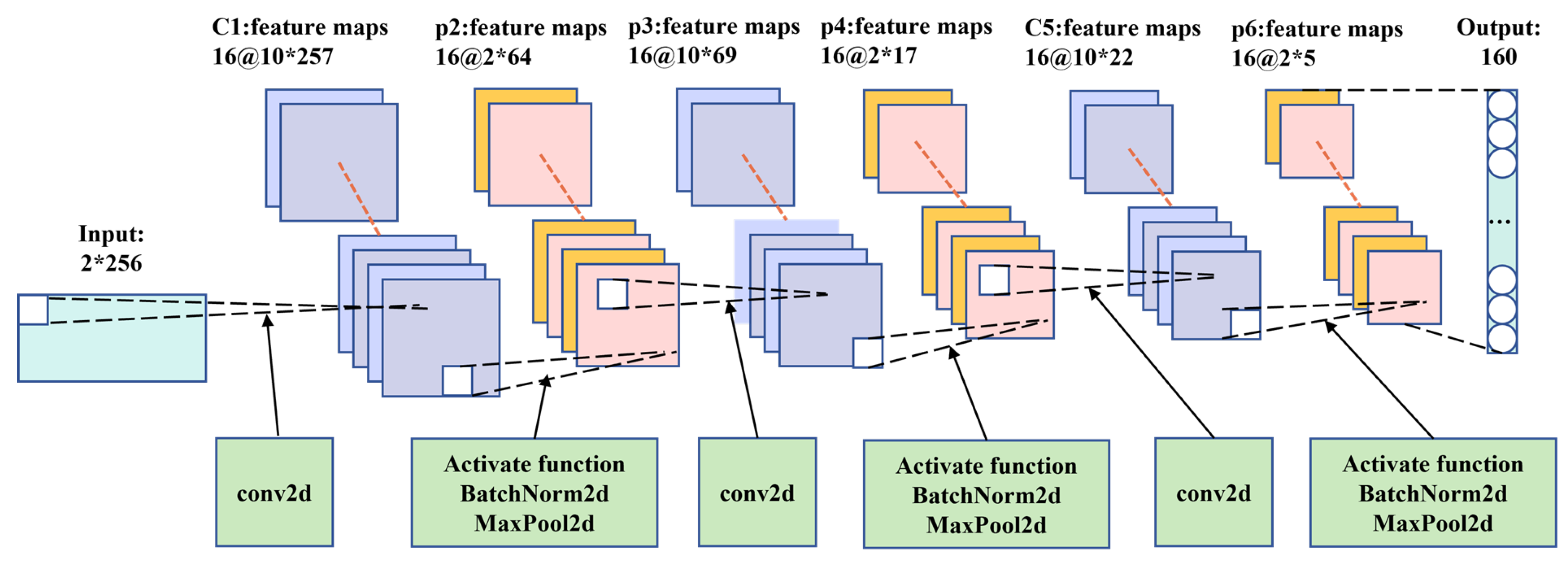
Figure 4.
The Bi-LSTM structure diagram provides a visual representation of the architecture and flow of information in a Bi-LSTM neural network.
Figure 4.
The Bi-LSTM structure diagram provides a visual representation of the architecture and flow of information in a Bi-LSTM neural network.
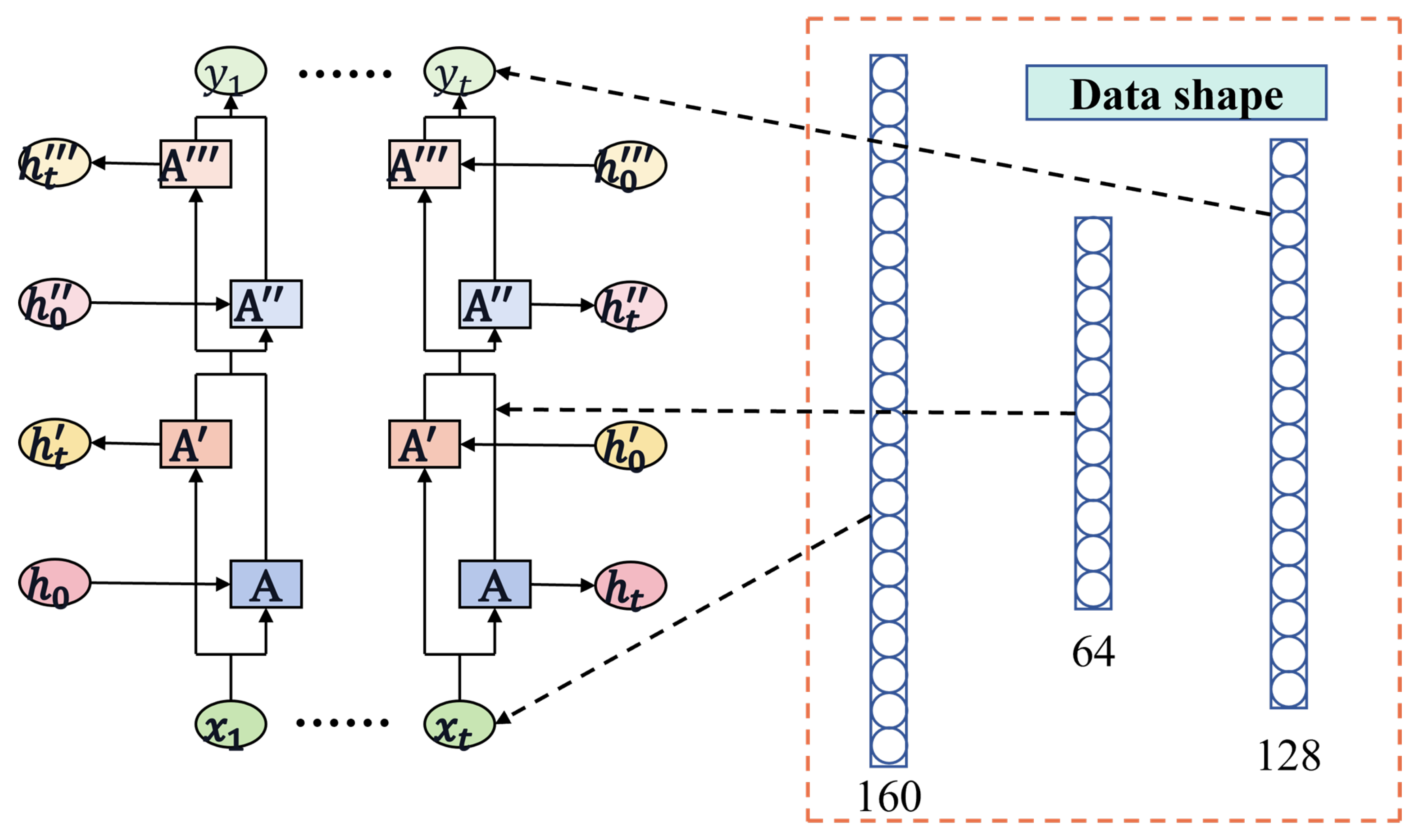
Figure 5.
The domain adaptation structure diagram clearly illustrates how to integrate domain adaptation modules on top of the existing network architecture.
Figure 5.
The domain adaptation structure diagram clearly illustrates how to integrate domain adaptation modules on top of the existing network architecture.
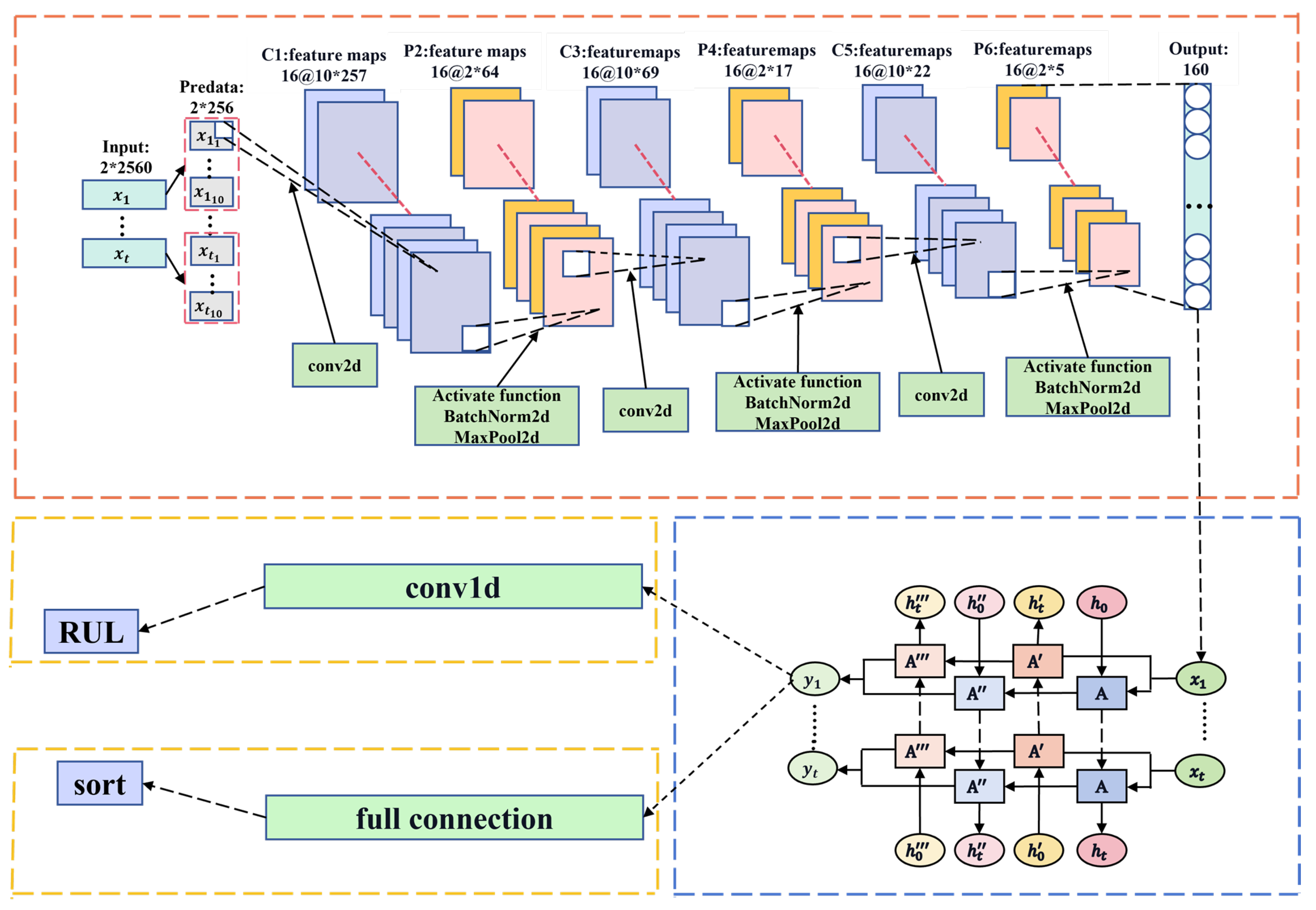
Figure 6.
Correlation accuracy of CNN model, where blue represents training set and red represents test set accuracy.
Figure 6.
Correlation accuracy of CNN model, where blue represents training set and red represents test set accuracy.
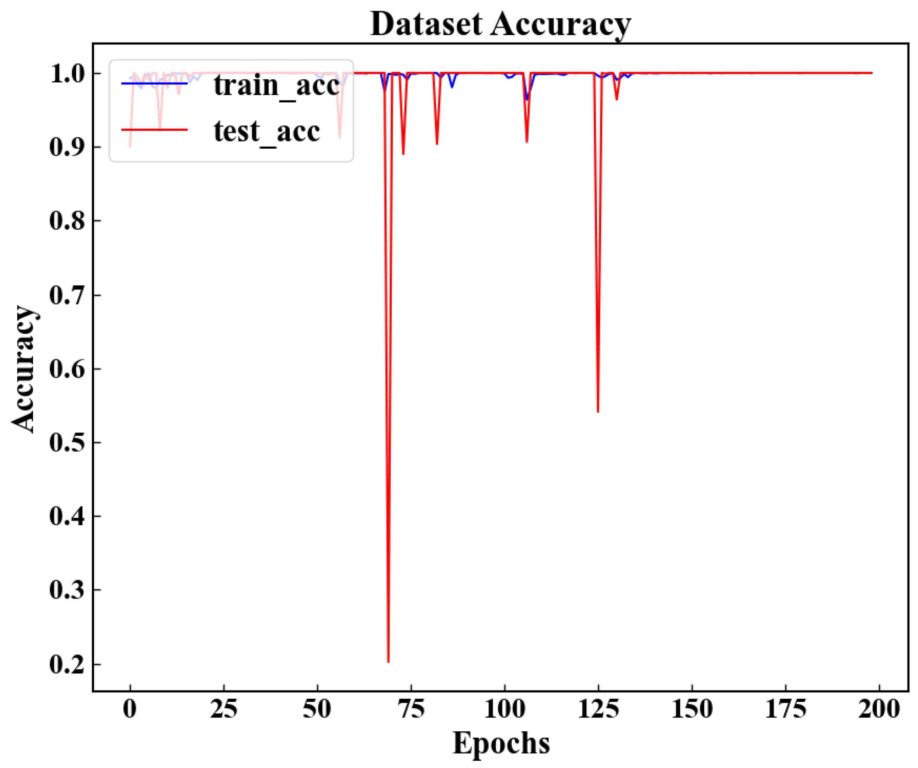
Figure 7.
The amplitude of the raw data, where the red circle represents the FOT points.(a-g expression Bearing1_1-1_7 amplitudes and fots.)
Figure 7.
The amplitude of the raw data, where the red circle represents the FOT points.(a-g expression Bearing1_1-1_7 amplitudes and fots.)
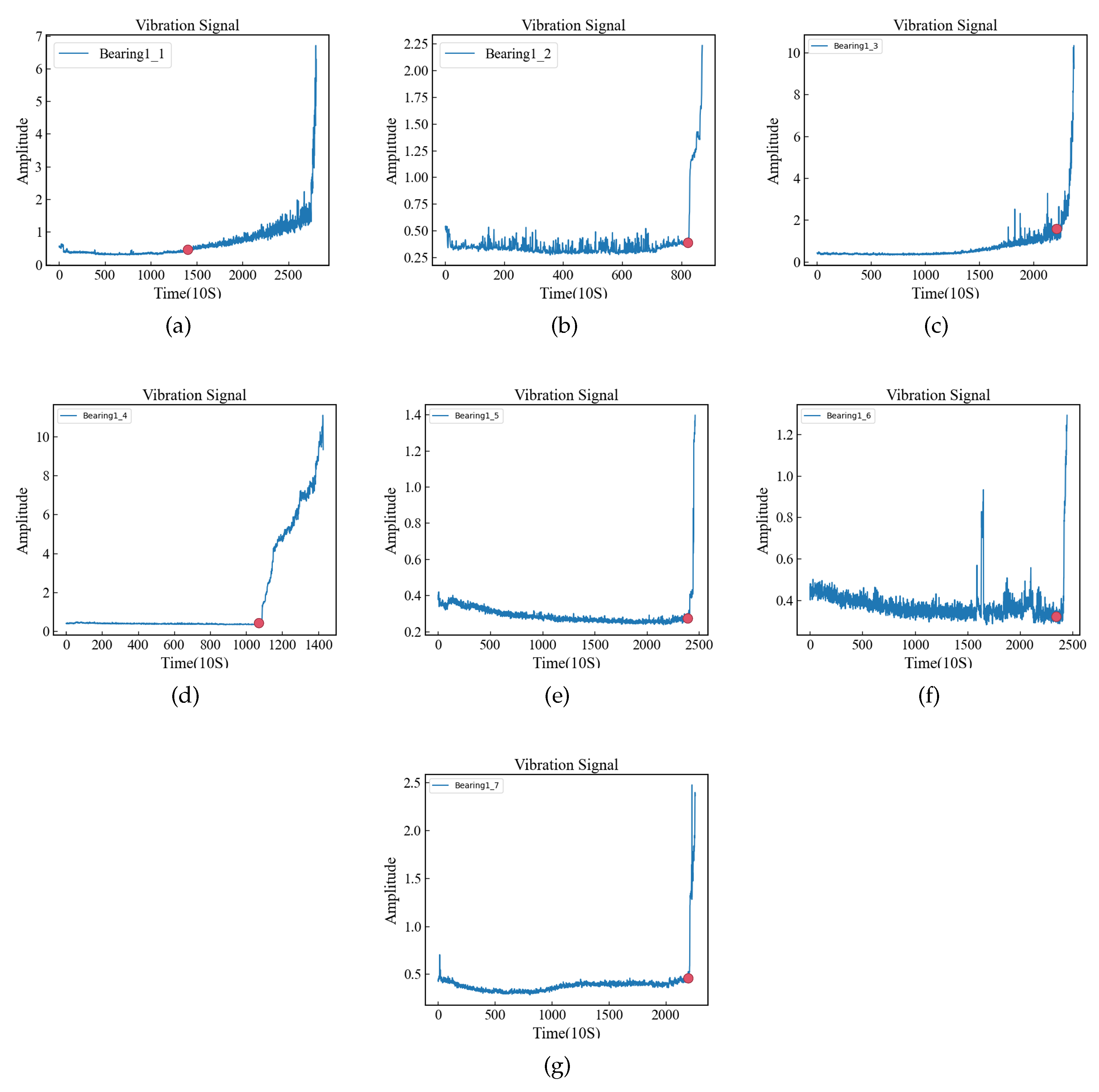
Figure 8.
The model predicted values, where the red dots represent FOT points based on amplitude and the yellow dots represent FOT points based on [10].(a-c expression Bearing1_5, Bearing1_6, Bearing1_7 predict_labels and fots.)
Figure 8.
The model predicted values, where the red dots represent FOT points based on amplitude and the yellow dots represent FOT points based on [10].(a-c expression Bearing1_5, Bearing1_6, Bearing1_7 predict_labels and fots.)

Figure 9.
For RUL prediction under various conditions, Bearing1_1 and Bearing1_2 under OC1 are used as training sets. The test set is as follows: Bearing1_3 and Bearing1_4 under OC1, Bearing2_1 and Bearing2_2 under OC2, and Bearing3_1 and Bearing3_2 under OC3 (corresponding to a-h in the figure). The yellow line indicates the predicted RUL, the blue line indicates the actual RUL, and the red line indicates the end of life.(a-h expression Bearing1_1, 1_2, 1_3, 1_4, 2_1, 2_2, 3_1, 3_2 RUL)

Figure 10.
Feature distribution of samples in different OCs. Each test group (Bearing1_3, Beqaring1_4, Bearing2_1, Bearing2_2, Bearing3_1, and Bearing3_2) was compared with training groups (Bearing1_1 and Bearing1_2). Samples in the same OC are compared in one subfigure.Red box lines indicate similar feature areas.
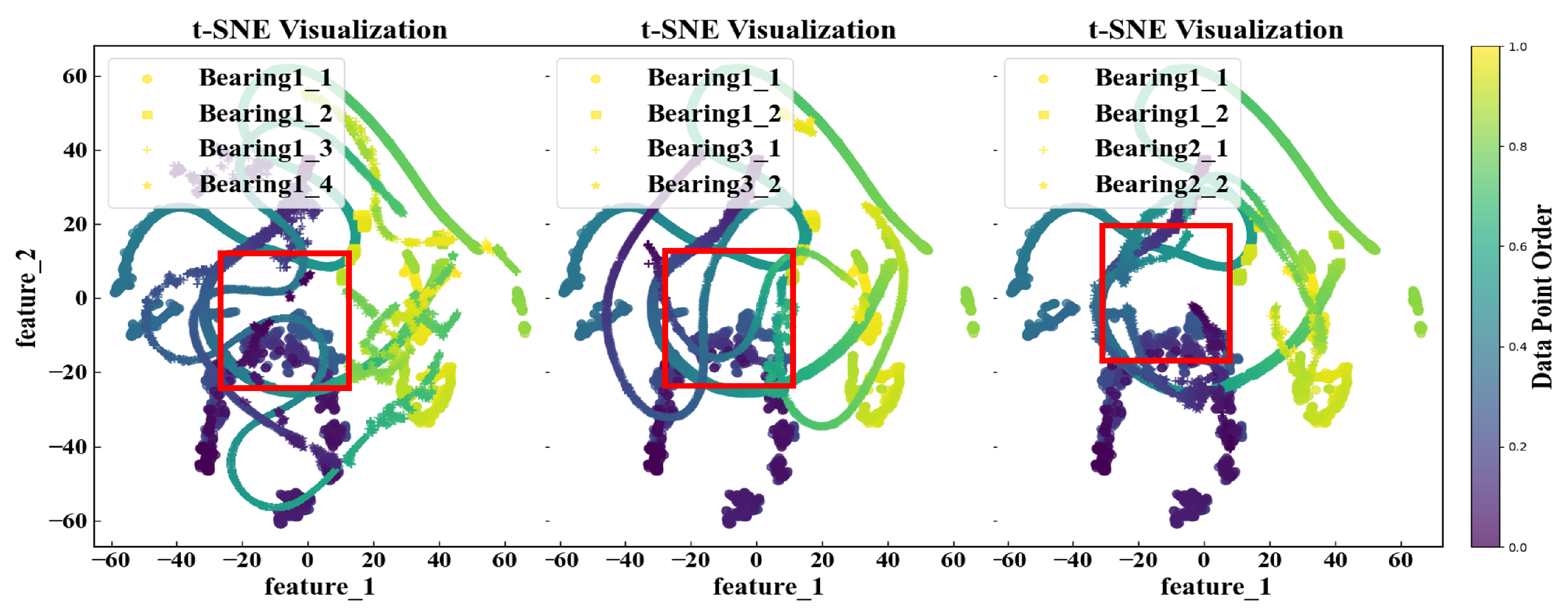
Table 1.
Datasets of IEEE 2012 PHM prognostic challenge.
| Operating Conditions | |||
|---|---|---|---|
| Datasets | Conditions 1 | Conditions 2 | Conditions 3 |
| Learning set | Bearing1_1 | Bearing2_1 | Bearing3_1 |
| Bearing1_2 | Bearing2_2 | Bearing3_2 | |
| Test set | Bearing1_3 | Bearing2_3 | Bearing3_3 |
| Bearing1_4 | Bearing2_4 | ||
| Bearing1_5 | Bearing2_5 | ||
| Bearing1_6 | Bearing2_6 | ||
| Bearing1_7 | Bearing2_7 | ||
Table 2.
Number of sample points in dataset.
| Dataset Name | Sample Size | Uncollected Sample |
|---|---|---|
| Bearing1_1 | 2803 | 0 |
| Bearing1_2 | 871 | 0 |
| Bearing1_3 | 2375 | 573(5730s) |
| Bearing1_4 | 1428 | 34(339s) |
| Bearing1_5 | 2463 | 161(1610s) |
| Bearing1_6 | 2448 | 146(1460s) |
| Bearing1_7 | 2259 | 757(7570s) |
| Bearing2_1 | 911 | 0 |
| Bearing2_2 | 797 | 0 |
| Bearing2_3 | 1955 | 753(7530s) |
| Bearing2_4 | 751 | 139(1390s) |
| Bearing2_5 | 2311 | 309(309s) |
| Bearing2_6 | 701 | 129(1290s) |
| Bearing2_7 | 230 | 58(580s) |
| Bearing3_1 | 515 | 0 |
| Bearing3_2 | 1637 | 0 |
| Bearing3_3 | 434 | 82(820s) |
Table 3.
Parameters of the CNN.
| Experimental parameter | Grid search related parameters | Final Numerical value | ||
|---|---|---|---|---|
| Optimizer | Adam | Adam | ||
| Learning_rate | 0.01 | 0.001 | 0.0001 | 0.01 |
| Loss_function | CrossEntropyLoss | CrossEntropyLoss | ||
| Batch_size | 8 | 16 | 32 | 32 |
| Activation_function | ReLU | Leaky_ReLU | Tanh | ReLU |
| Number of iterations | 10 | 200 | ||
Table 4.
CRWU Dataset.
| Condition 1 | Condition 2 | Condition 3 | Condition 4 | |||||||||
|---|---|---|---|---|---|---|---|---|---|---|---|---|
| Breakdown | 0.007" | 0.014" | 0.021" | 0.007" | 0.014" | 0.021" | 0.007" | 0.014" | 0.021" | 0.007" | 0.014" | 0.021" |
| Inner | 105.mat | 169.mat | 209.mat | 106.mat | 170.mat | 210.mat | 107.mat | 171.mat | 211.mat | 108.mat | 172.mat | 212.mat |
| Ball | 118.mat | 185.mat | 222.mat | 119.mat | 186.mat | 223.mat | 120.mat | 187.mat | 224.mat | 121.mat | 188.mat | 225.mat |
| 130.mat | 197.mat | 234.mat | 131.mat | 198.mat | 235.mat | 132.mat | 199.mat | 236.mat | 133.mat | 200.mat | 237.mat | |
| Outer | 144.mat | 246.mat | 145.mat | 247.mat | 146.mat | 248.mat | 147.mat | 249.mat | ||||
| 156.mat | 258.mat | 158.mat | 259.mat | 159.mat | 260.mat | 160.mat | 261.mat | |||||
| Normal | 97.mat | 98.mat | 99.mat | 100.mat | ||||||||
Table 5.
Experimental data and results.
| Experimental parameter | Numerical value | Experimental parameter | Numerical value |
|---|---|---|---|
| Total_data | Condition 1 all data | Train_data | 0.7*total_data |
| Test_data_1 | 0.3*total_data | Test_data_2 | Condition 2 all data |
| Test_data_3 | Condition 3 all data | Test_data_4 | Condition 4 all data |
| Test_data_1_acc_rate | 1.0 | Test_data_2_acc_rate | 1:1.0,0:0.961 |
| Test_data_3_acc_rate | 1:1.0,0:0.885 | Test_data_4_acc_rate | 1:1.0,0:0.698 |
Table 6.
FOT of Dataset
| Bearing | Sample Size | FOT([10]) | FOT(Amplitude) |
|---|---|---|---|
| 1_1 | 2803 | 1490 | 1490 |
| 1_2 | 871 | 827 | 827 |
| 1_3 | 2375 | 1684 | 2200 |
| 1_4 | 1428 | 1083 | 1080 |
| 1_5 | 2463 | 680 | 2400 |
| 1_6 | 2448 | 649 | 2400 |
| 1_7 | 2259 | 1026 | 2200 |
Table 7.
ACC of Dataset
| Bearing | ACC_rate([10]) | ACC_rate(Amplitude) |
|---|---|---|
| 1_1 | 0.9697 | 0.9697 |
| 1_2 | 0.9977 | 0.9977 |
| 1_3 | 0.7326 | 0.8025 |
| 1_4 | 0.8179 | 0.8172 |
| 1_5 | 0.3134 | 0.9704 |
| 1_6 | 0.4788 | 0.7496 |
| 1_7 | 0.4998 | 0.9398 |
Table 8.
Basic parameters of the model.
| Experimental parameter | Random search numerical value | Final numerical value | ||
|---|---|---|---|---|
| Optimizer | Adam | Adam | ||
| Learning_rate | 0.01 | 0.001 | 0.0001 | 0.001 |
| Loss_function | MSELoss | MSELoss | ||
| Num_layers | 1 | 2 | 3 | 2 |
| Hidden_size | 64 | 128 | 256 | 64 |
| Input_size | 160 | 160 | ||
| Batch_size | 16 | 32 | 64 | 32 |
| Number of iterations | 10 | 200 | ||
| Activation_function | ReLU | Leaky_ReLU | Tanh | ReLU |
Table 9.
Basic model evaluation metrics and evaluation indices for I-DCNN and MCNN.
| Proposed | I-DCNN | MCNN | ||||
|---|---|---|---|---|---|---|
| Bearing | MAE | RMSE | MAE | RMSE | MAE | RMSE |
| 1_3 | 0.1112 | 0.1370 | 0.2190 | 0.2513 | / | / |
| 1_4 | 0.1325 | 0.1840 | 0.4865 | 0.5236 | / | / |
| 1_5 | 0.1921 | 0.2341 | 0.1949 | 0.2199 | / | / |
| 1_6 | 0.1712 | 0.2035 | 0.1734 | 0.2002 | / | / |
| 1_7 | 0.1790 | 0.2024 | 0.2145 | 0.2499 | / | / |
| NRMSE | 0.1922 | 0.2890 | 0.3805 | |||
Table 10.
Comparative analysis of the performance of various time series models.
| Bi-LSTM | LSTM | RNN | Bi-RNN | GRU | Bi-GRU | |||||||
|---|---|---|---|---|---|---|---|---|---|---|---|---|
| Bearing | NMAE | NRMSE | NMAE | NRMSE | NMAE | NRMSE | NMAE | NRMSE | NMAE | NRMSE | NMAE | NRMSE |
| OC1 | 0.1020 | 0.1576 | 0.2346 | 0.2735 | 0.2433 | 0.2869 | 0.2788 | 0.3369 | 0.2723 | 0.3285 | 0.1274 | 0.1641 |
| OC2 | 0.2036 | 0.2235 | 0.2268 | 0.2661 | 0.2386 | 0.2840 | 0.2815 | 0.3414 | 0.2904 | 0.3420 | 0.1831 | 0.7728 |
| OC3 | 0.1795 | 0.2152 | 0.2399 | 0.2785 | 0.2464 | 0.2891 | 0.2770 | 0.3343 | 0.3343 | 0.3832 | 0.1621 | 0.2037 |
Table 11.
Jensen–Shannon divergence of baseline feature distribution.
| Feature region | JS divergence(Bearing1_1) | JS divergence(Bearing1_2) |
|---|---|---|
| Bearing1_1 | / | 0.1494 |
| Bearing1_2 | 0.1494 | / |
| Bearing1_3 | 0.6848 | 0.0837 |
| Bearing1_4 | 0.4578 | 0.2097 |
| Bearing2_1 | 0.4416 | 0.1500 |
| Bearing2_2 | 0.6364 | 0.1249 |
| Bearing3_1 | 0.8425 | 0.1065 |
| Bearing3_2 | 0.5660 | 0.0663 |
Table 12.
Basic parameters of domain adaption experiment.
| Experimental parameter | Numerical value |
|---|---|
| Optimizer | Adam |
| Learning rate | 0.0001 |
| Predict loss function | MSELoss |
| Domain loss function | CrossEntropyLoss |
| Num_layers | 2 |
| Hidden_size | 64 |
| Input_size | 160 |
| Batch_size | 32 |
| Number of iterations | 200 |
| Source domain data set | Bearing1_1 |
| Target domain data set | Bearing2_1,Bearing2_2,Bearing3_1,Bearing3_2 |
Table 13.
Domain adaption model and original model evaluation index.
| Domain_model | Raw_model | |||
|---|---|---|---|---|
| Bearing | MAE | RMSE | MAE | RMSE |
| 1_1 | 0.0419 | 0.0578 | 0.0511 | 0.0662 |
| 2_1 | 0.2996 | 0.3572 | 0.3007 | 0.3634 |
| 2_2 | 0.2027 | 0.2500 | 0.1964 | 0.2444 |
| 3_1 | 0.1833 | 0.2274 | 0.1880 | 0.2353 |
| 3_2 | 0.1917 | 0.2274 | 0.1955 | 0.2316 |
Disclaimer/Publisher’s Note: The statements, opinions and data contained in all publications are solely those of the individual author(s) and contributor(s) and not of MDPI and/or the editor(s). MDPI and/or the editor(s) disclaim responsibility for any injury to people or property resulting from any ideas, methods, instructions or products referred to in the content. |
© 2024 by the authors. Licensee MDPI, Basel, Switzerland. This article is an open access article distributed under the terms and conditions of the Creative Commons Attribution (CC BY) license (http://creativecommons.org/licenses/by/4.0/).
Copyright: This open access article is published under a Creative Commons CC BY 4.0 license, which permit the free download, distribution, and reuse, provided that the author and preprint are cited in any reuse.


