Remaining Useful Life Prediction in Varied Operational Conditions Considering Change Point: A Novel Deep Learning Approach with Optimum Features

1. Introduction

In today's Artificial Intelligence (AI)-driven advanced technological era, particularly in the field of aviation, ensuring the reliability, availability, and performance of aircraft systems is crucial to prevent unexpected failures, malfunctioning, and breakdowns[1]. One of the most important techniques in achieving this objective is the accurate prediction of RUL value of turbofan engines[2]. Gradual degradation of reliability and performance of a turbofan engine is a natural phenomenon. Sensors are used to understand such degradation patterns as well as to track machine conditions through a machine health index value. This index value is used to predict RUL value[3,4]. The RUL prediction offers confidence to the aircraft engineers on how long the engine or its components will continue to operate effectively before reaching a critical state. The accurate estimation of RUL serves as a proactive approach in optimal aircraft maintenance, enabling timely interventions and thereby preventing any untoward incidences of the engine[5,6]. Aviation engineers and maintenance personnel can plan and execute maintenance activities optimally by accurately foreseeing the point at which components might degrade or fail. This predictive maintenance strategy avoids unplanned downtime, enhances safety, and contributes to a more cost-effective and streamlined operational processes[7,8,9].

Due to the rapid advancements in IoT-based sensor technology, a wide array of sensors is now employed to monitor the operational health of turbofan engines[10]. Leveraging sensor-generated data, researchers have recently developed different data-driven models to forecast the RUL of these turbofan engines[5,11]. A hybrid Autoregressive Integrated Moving Average-Support Vector Machine (ARIMA-SVM) model was proposed by Ordonez et al.[12] for RUL prediction. In this study, the ARIMA model has been used to forecast sensor signals over time, and the SVM model was used later to predict RUL using the predicted sensor signals. Wang et al.[13] developed a Hidden Markov Model (HMM) for RUL prediction. A data-driven model was developed by Liu et al.[14] considering various sensor data to predict sensor anomaly and RUL of various complex machines. A fuzzy inference system (FIS)-based model was developed by Wu et al.[15] to predict the RUL of different matching tools. Wu et al.[16] utilized an extreme machine learning model to predict the RUL of lithium-ion battery. Li et al.[17] developed a convolution neural network (CNN)-based model to achieve better accuracy of RUL prediction. In this study, different time series models were used to predict the Sensor signals, and then the CNN model was used based on these predicted sensor signals to predict the RUL. A modified deep CNN model was proposed by Li et al.[18] for RUL prediction. Most of these studies considered all available sensor-based data for RUL prediction. However, not all sensors have similar importance in RUL prediction. Therefore, it is important to consider the most relevant sensors through feature engineering techniques for RUL prediction.

The primary challenge in performance degradation monitoring, machine health checking, and RUL prediction involves deriving important features from raw data collected from sensors [19]. Generally, various sensors are used to collect information related to time-domain and frequency-domain-based features with the assumption of a stationary degradation model until a fault occurs. However, these features might only be effective during specific operational stages, posing limitations. Additionally, modern machineries often function under diverse operating conditions, complicating the extraction of representative features. Variations in operating conditions can lead to distinct degradation models for the same machine, reflecting data dynamics and challenging the usability of conventional stationary features [20]. One prevalent approach to tackle this challenge is the utilization of feature engineering methods tailored to degradation patterns in the data. These methods aim at extracting more relevant features capable of accommodating different operating conditions. Kundu et al.[21] proposed a Weibull Accelerated Failure Time Regression (WAFTR) model specifically designed to extract representative features under various conditions. Wang and Zhao[20] also designed a three-step-based feature selection method to select important features before prediction of RUL. Buchaiah and shakya[22] proposed a RUL prediction algorithm based on Bhattacharyya distance and SVM techniques. A random forest algorithm was initially developed in this study for important feature selection, which helped to achieve better accuracy in RUL prediction for turbofan engines. Most of these developed methodologies for RUL prediction have assumed uniform operating conditions following similar and systematic patterns of RUL, which may not be the case in reality. Therefore, there is a need to develop a RUL-prediction model considering such changes in operating and environmental conditions.

Changes in the basic levels of operating conditions, environments, and skills to operate and maintain an engine, with their respective fluctuations around the levels, are expected to change the trend and pattern of RUL. In this context, the alteration in RUL patterns is identified as a change point[23]. Finding the exact location of the change point helps to estimate the RUL more accurately. Therefore, change point detection has recently become a significant and crucial problem for RUL estimation. Detecting change point in RUL prediction involves analyzing various data obtained from sensors or monitoring systems attached to the equipment. Wen et al.[24] proposed a model initially to predict the change point location in RUL. A dual-long short-term memory (LSTM) model was also developed by Shi and Chehade[25] to find the location of change point in RUL. In this study, they showed the performance of their developed model is better than baseline deep learning models. The identification of these change point locations allows predictive maintenance models to adapt or be revised in response to the machinery's evolving behaviour, thereby enhancing the accuracy of RUL estimations.

Turbofan engine, with its multi-dimensional complexity and dynamics, makes it extremely difficult to predict its health condition and RUL. Therefore, deep neural network models are more suitable for prediction than classical machine learning models, and the same is discussed in recent literatures[17,18,26,27,28,29,30]. Among various deep learning models, Bidirectional Long Short-Term Memory networks (BiLSTMs) hold significant importance in time series data modelling, especially in tasks requiring context from past and future information[31]. BiLSTMs offer advantages over traditional LSTM networks and other Recurrent Neural Networks (RNN) as they can simultaneously capture information from preceding and succeeding sequences, diminish information loss during network training, and model long-term dependencies in sequential data[32]. In this article, a BiLSTM network has been developed to predict RUL for turbofan engines. For RUL prediction, initially a feature selection algorithm has been proposed in this article to identify crucial features from a pool of sensor data. This algorithm not only discerns important features but also tracks the weights of these features, aiding in subsequent RUL prediction. It acts as a filter, eliminating unnecessary sensor signals for accurate RUL prediction. An algorithm for change point detection has also been proposed here based on the selected features to identify the change point location for every engine. This change point analysis, conducted on the chosen features, significantly contributes to RUL prediction in this study. Finally, a BiLSTM model has been proposed here based on selected sensors and change points to predict the health index as well as the RUL value of turbofan engines. The main contributions of the paper can be summarized as follows:

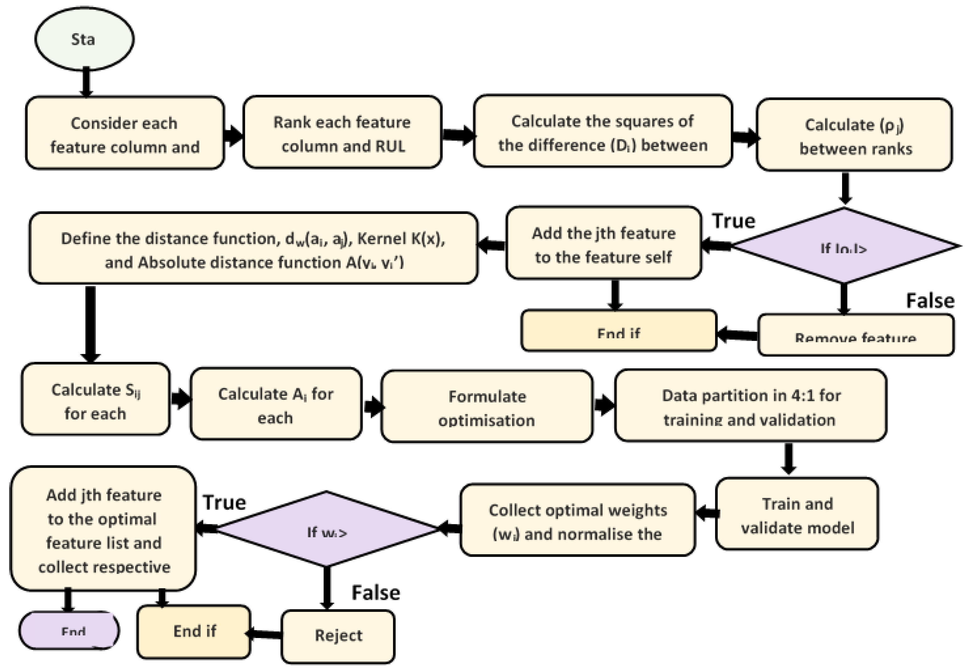
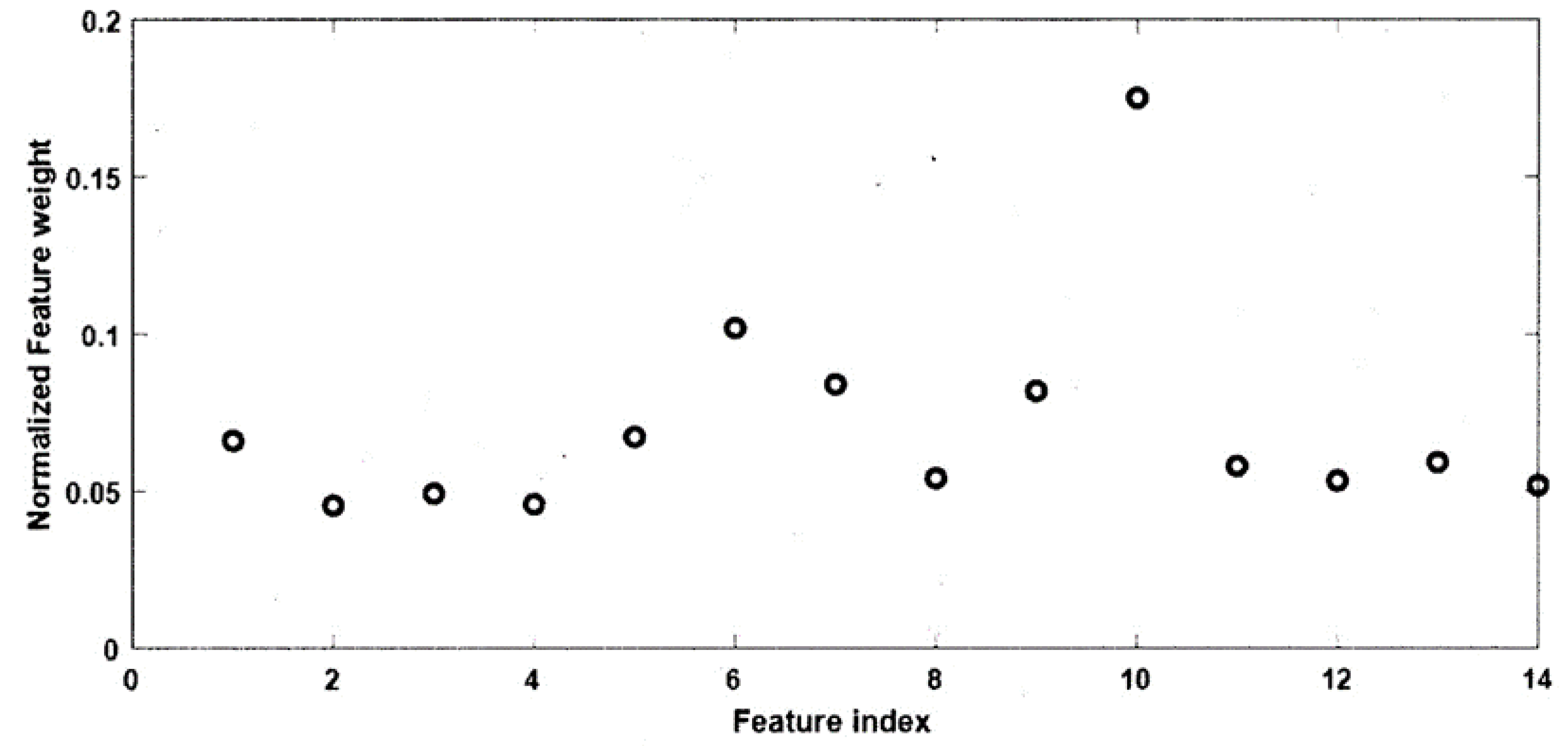
• Proposing a new feature selection algorithm to identify the most important features from all sensor data for RUL prediction. This proposed algorithm also keeps track of the feature weight corresponding to each important feature, which helps to predict the RUL later. The feature selection algorithm is a prerequisite to filter out the unnecessary sensor signals for RUL prediction.
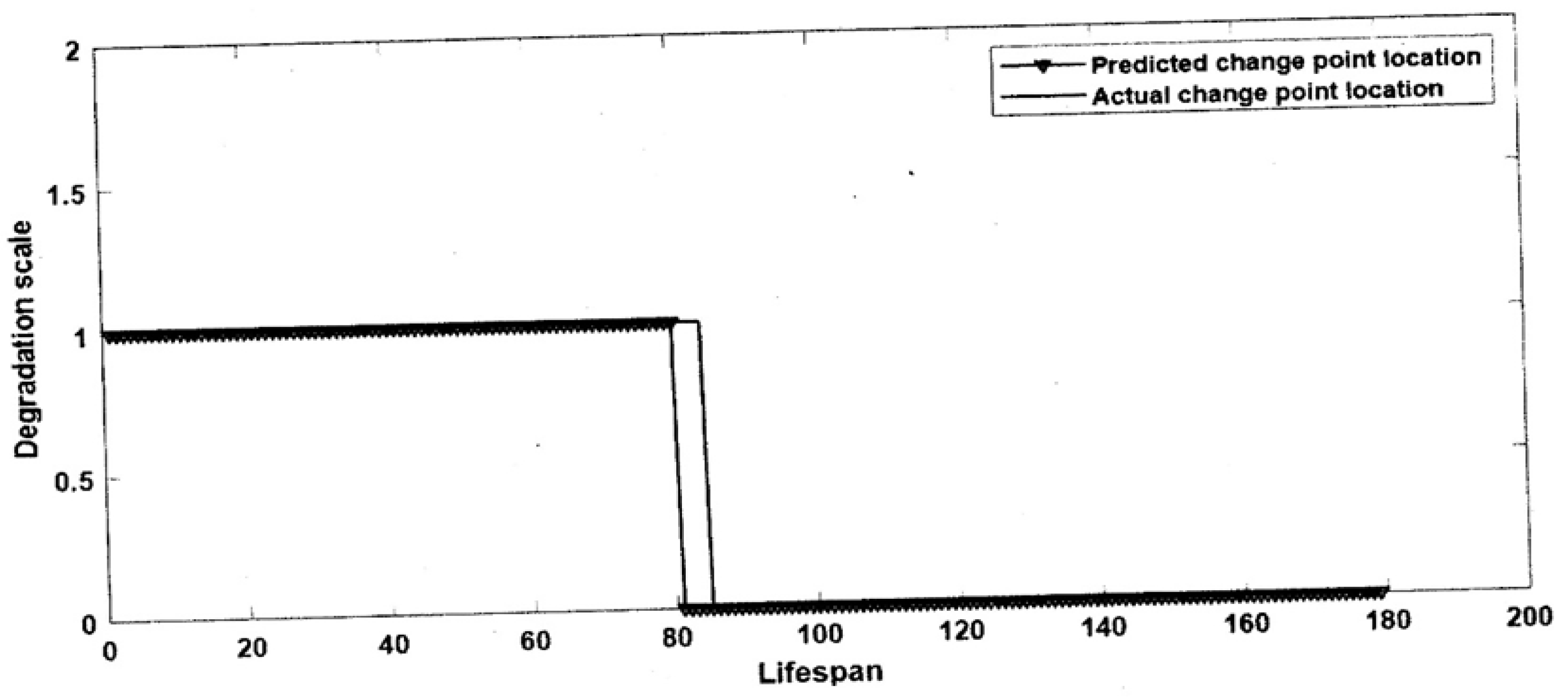
• Introducing a logistic regression-based algorithm for change point detection for each engine on the basis of their respective selected important features.
• Designing a BiLSTM network for prediction of RUL with the optimal number of sensors so that both long-term and short-term dependencies within the sensor can be characterized bidirectionally via the BiLSTM network. Therefore, historical information can be preserved as much as possible and used for health index as well as RUL prediction.
• Demonstrating the superior performance of the proposed methodology on the basis of C-MAPSS data and comparing the performances with some existing models.

Before delving into the specifics of the paper, structural flow in this article is outlined in five sections. Having introduced the study in section 1, the subsequent sections have been laid out. Section 2 provides the essential backgrounds and related mathematical formulations needed for this study. The details of the proposed methodology are described in Section 3. Section 4 demonstrates the experimental setup and performance comparison of the proposed methodology against existing models, and finally, Section 5 offers concluding remarks.

2. Prerequisites

This section introduces some mathematical and other theoretical background knowledge and information required to develop the proposed model of RUL prediction. In this study, a special kind of Recurrent Neural Network (RNN) network called Bidirectional Long short-term memory (BiLSTM) has been used for RUL prediction. Details of different deep learning techniques like: Recurrent Neural Network (RNN), Long short-term memory (LSTM), and Bidirectional Long short-term memory (BiLSTM) have been described in this section.

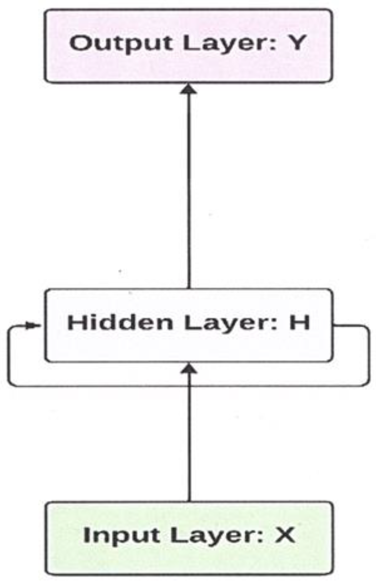
2.1. Recurrent Neural Network (RNN)

Recurrent neural networks (RNNs) are the extensions of conventional feed-forward neural networks, which can take care of sequence data. Unlike a unidirectional feed forward neural network, a bidirectional artificial neural network permits information to flow in both forward and backward directions[33]. That indicates the output from certain nodes can influence subsequent input to the succeeding nodes in a network environment. Capability of the network utilizes internal memory to handle various sequences of inputs suitably for the prediction of different tasks such as handwriting recognition, speech recognition, etc. The pictorial representation of an RNN model has been given in Figure 1. A formal definition of RNN can be given as follows:

Let us assume ${\mathrm{a}}^{\mathrm{t}}=({\mathrm{a}}_1^{\mathrm{t}},{\mathrm{a}}_2^{\mathrm{t}},...,{\mathrm{a}}_{\mathrm{t}}^{\mathrm{t}},\mathrm{...},{\mathrm{a}}_{\mathrm{T}}^{\mathrm{t}})$ represents input vectors with length T and ${\mathrm{k}}_{\mathrm{t}}$represents RNN memory at time step t. Then, RNN can be updated its memory with the formula using:

$${\mathrm{k}}_{\mathrm{t}}=\mathrm{\alpha }({\mathrm{S}}_{\mathrm{x}}.{\mathrm{a}}_{\mathrm{t}}+{\mathrm{S}}_{\mathrm{h}}{\mathrm{k}}_{\mathrm{t}-1}+{\mathrm{b}}_{\mathrm{t}})$$

(1)

where$\mathrm{\alpha }(\mathrm{p})$is a nonlinear activation function (e.g., logistic sigmoid function or hyperbolic tangent function), ${\mathrm{S}}_{\mathrm{x}},{\mathrm{S}}_{\mathrm{h}}$are weight matrices, and${\mathrm{b}}_{\mathrm{t}}$is a constant bias for time stamp t.

Generally, two problems can be looked at while training a RNN model; one is known as “vanishing gradients”, and the other is known as “exploding gradients”. The information passes through many layers, and it will vanish or wash out by the time it reaches the last layer or the first layer. This phenomenon is called as “vanishing gradients”. On the other hand, “exploding gradients” refers to the cases in which information about the gradient becomes large when it passes through a lot of layers. It will then result in a very high gradient when it reaches to the last layer or first layer. These problems make it hard to train the network. These problems can be solved by truncating or squashing the gradients[25].

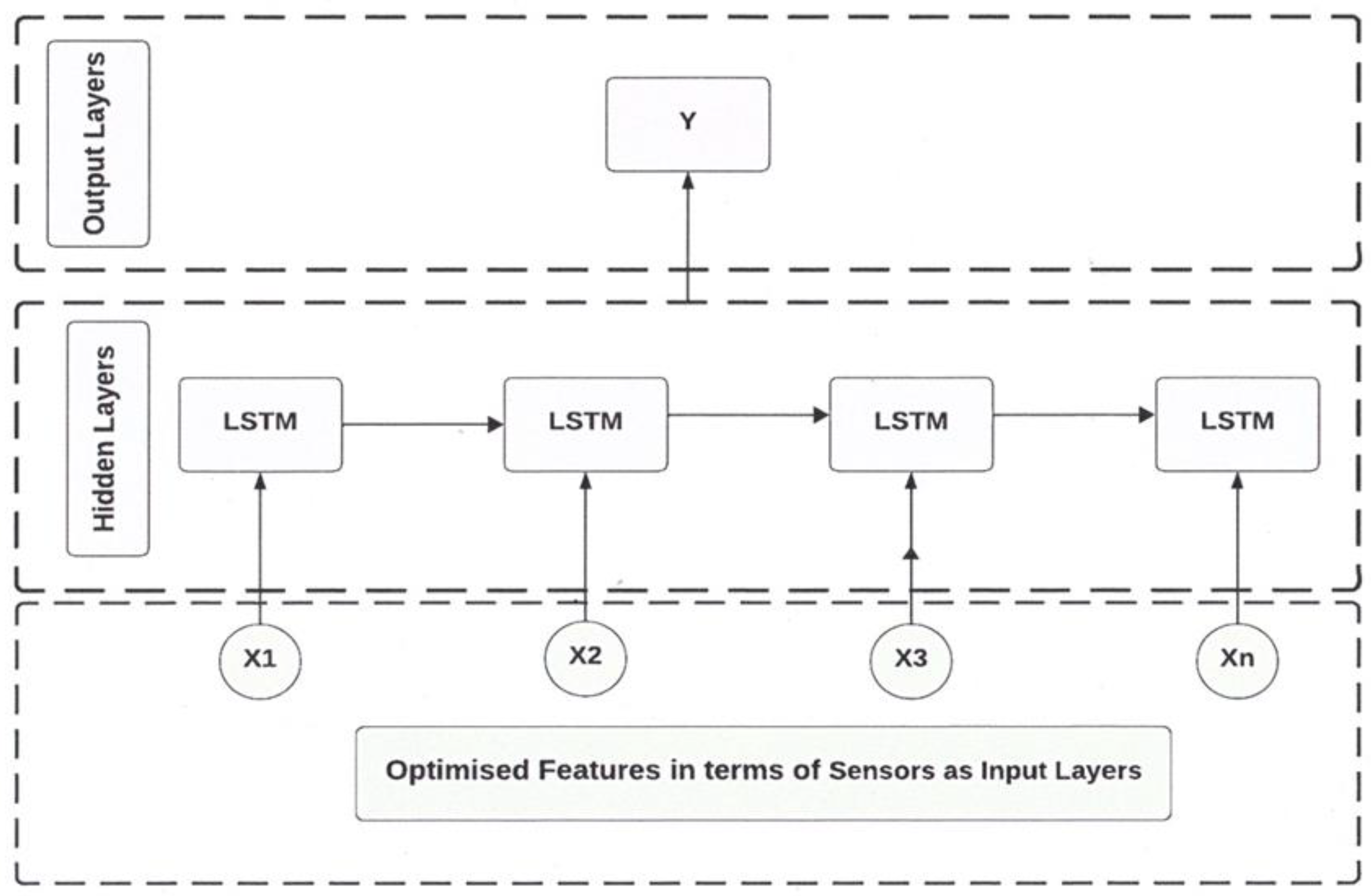
2.2. Long-Short Term Memory (LSTM)

Due to difficulties created during training RNNs, a new RNN technique called long short-term memory (LSTM) model was developed to tackle the long-term dependencies of input data by Hochreiter and Schmidhuber in 1997[34]. LSTM model is an extension of the RNN model developed to address the vanishing gradient problem. The LSTM memory is called a “Gated” cell, where the decision to preserve or ignore of the information is made. An LSTM model takes the information from the input features and keeps the information in the cell for a long period of time. The information, that is deleted from cell, is decided based on allocated weights on the features while training the model[35]. The architecture of the LSTM model is given in Figure 2.

The LSTM model generally consists of three gates like: “Forget gate”, “Input gate”, and “Output gate”.

2.2.1. Forget Gate

In this gate, a decision is taken for preserving or deleting information. The preserving or deleting the information depends on the allocated weights of the input features. A sigmoid function is used in this gate during training the LSTM model. The decision is made based on the values of ${\mathrm{k}}_{\mathrm{t}-1},{\mathrm{a}}_{\mathrm{t}}$. The output of the gate, ${\mathrm{M}}_{\mathrm{t}}$, lies between 0 and 1. Here, 0 indicates total forget about the feature and 1 implies preserving the whole information about the feature. Mathematically, the formula can be written as follows:

$${\mathrm{M}}_{\mathrm{t}}=\mathrm{\sigma }({\mathrm{S}}_{\mathrm{k}\mathrm{M}}[{\mathrm{k}}_{\mathrm{t}-1}],{\mathrm{S}}_{\mathrm{a}\mathrm{M}}[{\mathrm{a}}_{\mathrm{t}}],{\mathrm{b}}_{\mathrm{M}})$$

(2)

where $\mathrm{\sigma }$is the sigmoid activation function and ${\mathrm{b}}_{\mathrm{M}}$ is the bias.

2.2.2. Input Gate

In this gate, a decision is taken on whether new information is added or not in the LSTM memory. This gate contains two layers: one is the sigmoid layer, and the other is the tanh layer. Based on sigmoid layer, it is decided whether the information is required or not, and the tanh layer updates the memory by adding information related to important features. The outputs of these two layers are computed by the formula:

$${\mathrm{N}}_{\mathrm{t}}=\mathrm{\sigma }({\mathrm{S}}_{\mathrm{k}\mathrm{N}}[{\mathrm{k}}_{\mathrm{t}-1}],{\mathrm{S}}_{\mathrm{a}\mathrm{N}}[{\mathrm{a}}_{\mathrm{t}}],{\mathrm{b}}_{\mathrm{N}})$$

(3)

$$\mathrm{and} {{\mathrm{L}}_{\mathrm{t}}}^{*}=\tanh ({\mathrm{S}}_{\mathrm{k}}[{\mathrm{k}}_{\mathrm{t}-1}],{\mathrm{S}}_{\mathrm{a}}[{\mathrm{a}}_{\mathrm{t}}],{\mathrm{b}}_{\mathrm{L}})$$

(4)

where ${\mathrm{N}}_{\mathrm{t}}$represents whether the values are updated or not and ${\mathrm{L}}_{\mathrm{t}}$represents the new values that will be added to the memory. Here,${\mathrm{b}}_{\mathrm{N}}$and${\mathrm{b}}_{\mathrm{L}}$are the biases of the sigmoid and tanh layers respectively. Finally, the combination of these two layers is used to update the value in the LSTM memory. The formula used for the upgradation of the memory value is as follows:

$${\mathrm{L}}_{\mathrm{t}}={\mathrm{M}}_{\mathrm{t}}\times {\mathrm{L}}_{\mathrm{t}-1}+{\mathrm{N}}_{\mathrm{t}}\times {{\mathrm{L}}_{\mathrm{t}}}^{*}$$

(5)

where ${\mathrm{M}}_{\mathrm{t}}$ is the output of the forget layer, whose value lies between 0 and 1.

2.2.3. Output Gate

In this gate, two operations are performed. Initially, a sigmoid activation function is used to decide which specific features are going to contribute the output. A nonlinear tanh activation function is then used on the output of input layer, which values lie between -1 to 1. Finally, the result is multiplied by the output of the sigmoid layer of this gate. Mathematically, the formula can be written as follows:

$${\mathrm{O}}_{\mathrm{t}}=\mathrm{\sigma }({\mathrm{S}}_{\mathrm{k}\mathrm{O}}[{\mathrm{k}}_{\mathrm{t}-1}],{\mathrm{S}}_{\mathrm{a}\mathrm{O}}[{\mathrm{a}}_{\mathrm{t}}],{\mathrm{b}}_{\mathrm{O}})$$

(6)

$$\mathrm{and} {\mathrm{h}}_{\mathrm{t}}={\mathrm{O}}_{\mathrm{t}}\times \tanh ({\mathrm{L}}_{\mathrm{t}})$$

(7)

where ${\mathrm{b}}_{\mathrm{O}}$is the bias of the output layer,${\mathrm{O}}_{\mathrm{t}}$is the output value, and is the output representation as a value between -1 and 1. Due to increase in the interdependency of explanatory variables, capturing the context of future information becomes crucial with capturing the context of past information. LSTM model can capture only past information but not future information. To acknowledge this issue, a bidirectional LSTM model was developed later. The detailed architecture of the BiLSTM is given in the next subsection.

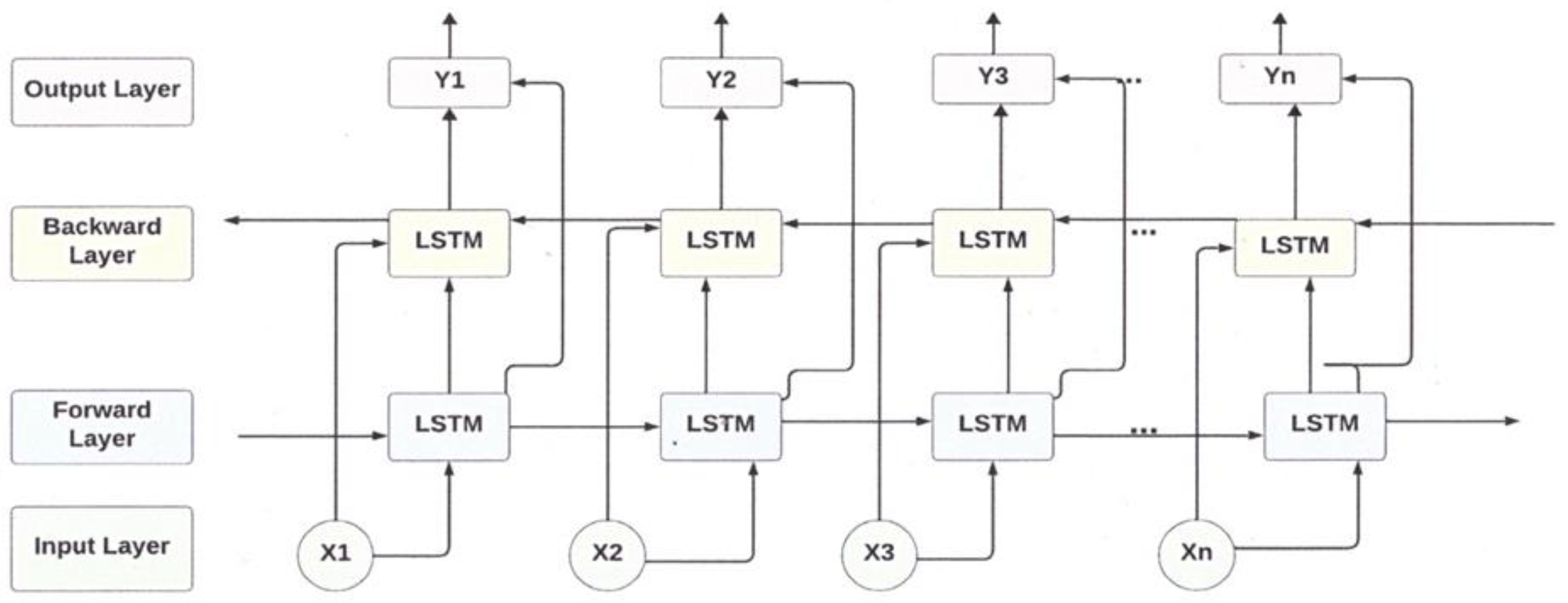
2.3. Bidirectional Long Short-Term Memory (BiLSTM)

The BiLSTM model is the extension of the LSTM model, which consists of two LSTM models[31]. The primary advantage of using a BiLSTM over an LSTM is its ability to capture context from past and future information and use it during testing. This bidirectional approach helps in understanding the context of a sequence more comprehensively, making it particularly useful in tasks where the complete context of the sequence matters, such as various time series prediction problems like predicting RUL in a machine. During BiLSTM model training, one LSTM model is trained as a forward layer, and the other LSTM model is trained as a backward layer to the input features. Applying two consecutive LSTMs helps to increase prediction accuracy[32]. An architecture of the BiLSTM model is given in Figure 3.

Figure 3 shows how two LSTM models work together in forward and backward layers for RUL prediction. The details of the proposed methodology have been discussed in the next section.

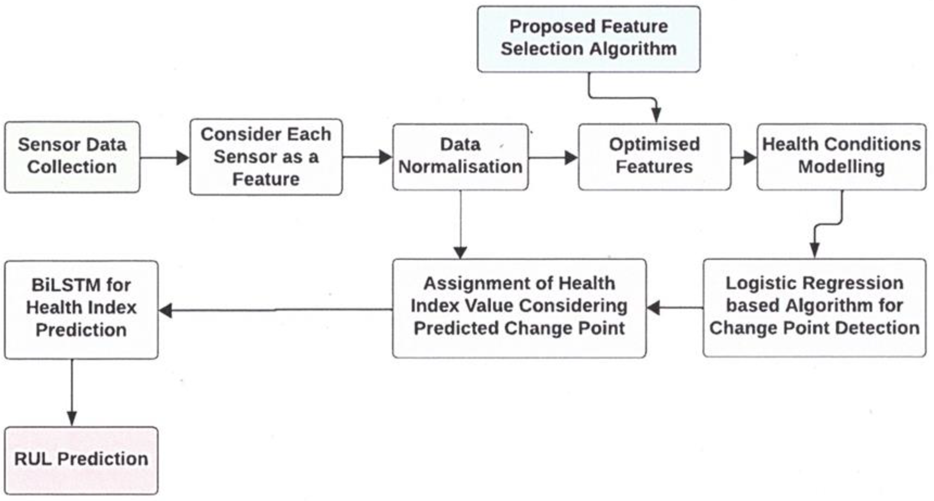
3. Proposed Methodology

A novel methodology has been proposed in this study to predict RUL value of turbofan engines. Collected data from various sensors are utilized as inputs for the RUL prediction. The proposed methodology consists of five steps are as under:

• normalization of the input features,
• optimal feature selection from all the sensors,
• change point detection for each turbofan engine,
• predict the health index of turbofan engines,
• RUL prediction based on the health index values for each turbofan engine.

Figure 4 depicts the workflow of the proposed methodology. The detailed steps of the proposed methodology have been described in the following subsections.

3.1. Feature Normalization

Incompatibility, inconsistency, and computational complexity in terms of measurement unit, values, and variations of features, to connect while relating the RUL values requires normalization of input features. This process also aids in outlier detection (if available), that is crucial for accurate RUL predictions. Therefore, a standard normalization formula is applied to input features for the development of RUL prediction model. In this study, the min-max rescaling technique is employed to normalize input vectors within the range of 0 to 1. Following the proposed methodology steps, the subsequent stage involves determining the most significant features from the pool of available features.

3.2. Feature Selection

Feature selection aims to consider only important features without compromising the prediction accuracy of the prediction model and reducing computational complexities. The emphasis is on removing redundant or noninformative variables that make negligible contributions to the performance of the RUL prediction model or might induce overfitting concerns. Pertaining to RUL prediction, the identification of the most pertinent features from sensor data aids in constructing predictive models capable of more precise estimations regarding the remaining life span of machines or systems. This subsequently enhances maintenance planning and the allocation of resources. This study introduces a two-stage-based methodology for feature selection, as elaborated in the proposed feature selection algorithm outlined in the next subsection. The progressive flow of development and working of the proposed model is available in Figure 5.

3.2.1. Proposed Two-Stage Feature Selection Algorithm

Input: Input feature set $\mathrm{D}=\{{\mathrm{S}}_{\mathrm{i}1},{\mathrm{S}}_{\mathrm{i}2},\mathrm{...},{\mathrm{S}}_{\mathrm{i}\mathrm{N}}\}$, $\mathrm{T}\mathrm{a}\mathrm{r}\mathrm{g}\mathrm{e}\mathrm{t} \mathrm{s}\mathrm{e}\mathrm{t}=\left\{\mathrm{R}\mathrm{U}{\mathrm{L}}_{\mathrm{i}}\right\}$ for $\mathrm{i}=1(1)\mathrm{n}.$Parameter: N: number of input features, n: number of total observations

Output: Optimized feature set $\mathrm{T}=[]\mathrm{a}\mathrm{n}\mathrm{d} \mathrm{F}\mathrm{W}=[];$

1^st step: Step for removal of irrelevant features

for j in 1: Total number of features (N)

Consider ${\mathrm{S}}_{\mathrm{j}}$and RUL columns

Sort and rank R${\mathrm{S}}_{\mathrm{j}}$and RUL columns

Calculate ${\mathrm{D}}_{\mathrm{i}}$= difference between two rank columns and ${{\mathrm{D}}_{\mathrm{i}}}^2$Calculate ${\mathrm{\rho }}_{\mathrm{j}}=1-{\displaystyle \frac{6\times {\displaystyle \sum _{\mathrm{i}=1}^{\mathrm{n}}{{\mathrm{D}}_{\mathrm{i}}}^2}}{\mathrm{n}({\mathrm{n}}^2-1)}}$if $\left|{\mathrm{\rho }}_{\mathrm{j}}\right|>0.05$Add ${\mathrm{S}}_{\mathrm{j}}$ to T and update T

Collect $\left|{\mathrm{\rho }}_{\mathrm{j}}\right|$ as weights and add to FW

else

Remove from the list

end

end

2^nd Step: Step for removal of redundant features and collect feature weights

Define ${\mathrm{d}}_{\mathrm{w}}({\mathrm{a}}_{\mathrm{i}},{\mathrm{a}}_{\mathrm{j}})={\displaystyle \sum _{\mathrm{r}=1}^{{\mathrm{N}}^{\prime }}{{\mathrm{w}}_{\mathrm{r}}}^2\{({\mathrm{x}}_{\mathrm{i}\mathrm{r}}-{\mathrm{x}}_{\mathrm{j}\mathrm{r}}){\sum }^{-1}{({\mathrm{x}}_{\mathrm{i}\mathrm{r}}-{\mathrm{x}}_{\mathrm{j}\mathrm{r}})}^{\mathrm{T}}\}}$ # where $\sum$is covariance matrix of input features and T is used for transpose of the matrix and w is weight matrix.

Define $\mathrm{k}(\mathrm{p})=\exp (-{\displaystyle \frac{\mathrm{p}}{\mathrm{\alpha }}})$ #

$\mathrm{\alpha }$is a constant

Define $\mathrm{A}({\mathrm{y}}_{\mathrm{i}},{\mathrm{y}}_{\mathrm{i}}\text{'})=|{\mathrm{y}}_{\mathrm{i}}-{\mathrm{y}}_{\mathrm{i}}\text{'}|$ # absolute distance between two points and ${\mathrm{y}}_{\mathrm{i}}\text{'}$is the output of multi-linear regression model

Input: N` is the number of features after removing irrelevant features

for i in 1 to n

for j in 1 to N`

$${\mathrm{S}}_{\mathrm{i}\mathrm{j}}={\displaystyle \frac{\mathrm{k}({\mathrm{d}}_{\mathrm{w}}({\mathrm{x}}_{\mathrm{i}},{\mathrm{x}}_{\mathrm{j}}))}{{\displaystyle \sum _{\mathrm{j}=1,\mathrm{j}\ne \mathrm{i}}^{\mathrm{N}`}\mathrm{k}({\mathrm{d}}_{\mathrm{w}}({\mathrm{x}}_{\mathrm{i}},{\mathrm{x}}_{\mathrm{j}}))}}}$$

end

$${\mathrm{A}}_{\mathrm{i}}={\displaystyle \sum _{\mathrm{j}=1,\mathrm{j}\ne \mathrm{i}}^{\mathrm{N}\text{'}}{\mathrm{S}}_{\mathrm{i}\mathrm{j}}.\mathrm{A}(\mathrm{R}\mathrm{U}{\mathrm{L}}_{\mathrm{i}},\mathrm{R}\mathrm{U}{\mathrm{L}}_{\mathrm{j}})}$$

Formation of optimization function: $\mathrm{f}(\mathrm{w})={\displaystyle \frac{1}{\mathrm{n}}}\times {\displaystyle \sum _{\mathrm{i}=1}^{\mathrm{n}}{\mathrm{l}}_{\mathrm{i}}+\mathrm{\chi }{\displaystyle \sum _{\mathrm{r}=1}^{\mathrm{N}\text{'}}{{\mathrm{w}}_{\mathrm{r}}}^2}}$ # Consider weight matrix of previous step

end

Divide training data in 5-parts for model training and validation

Train f(w) based on 4 parts and validate on 1 part

for j in 1 to N’

Collect weights ${\mathrm{w}}_{\mathrm{j}}$ from optimized model

$${\mathrm{w}}_{\mathrm{j}}={\displaystyle \frac{{\mathrm{w}}_{\mathrm{j}}}{{\displaystyle \sum _{\mathrm{j}}{\mathrm{w}}_{\mathrm{j}}}}}$$

end

Optimized feature set$=\mathrm{O}\mathrm{F}=[]$ and normalized weight$=\mathrm{N}\mathrm{W}=[]$.

if ${\mathrm{w}}_{\mathrm{j}}>0.04$ Add ${\mathrm{S}}_{\mathrm{j}}$ in OF and collect ${\mathrm{w}}_{\mathrm{j}}$ and store in NW.

else

Remove as redundant feature

end

This proposed algorithm helps collect optimal features and the weights (in normalized form) corresponding to each selected feature, which influence the health condition and RUL value of the turbofan engines. Following the feature selection process, the subsequent subsection conducts a change point analysis based on the chosen features.

3.3. Change Point Detection

As the flowchart of the proposed methodology in Figure 4 shows, once the data with optimal features are fully prepared, the third step is to detect the change point for each engine based on the multi-sensor data. Machines or equipment may operate under changing conditions, prompting the need to detect shifts or changes in their operational context, such as variations in operating conditions, maintenance activities, or external influences. Detecting these change points allows for adjustments or updates to predictive maintenance models to accommodate the evolving behaviour of the machinery. In this study, a change point analysis has been conducted for RUL prediction. The sensors, selected through the proposed feature selection algorithm, serve as input for the change point detection process. A logistic regression model has been trained to pinpoint the change point location for each Turbofan engine.

At time t, the input ${\mathrm{a}}_{\mathrm{t}}=[{{\mathrm{a}}_{\mathrm{t}}}^{(1)},{{\mathrm{a}}_{\mathrm{t}}}^{(2)},\mathrm{....},{{\mathrm{a}}_{\mathrm{t}}}^{(\mathrm{N}\text{'})}]$represents the normalized sensor data, where N’ is the optimal number of features selected based on the proposed feature selection algorithm. If m is the number time stamps, ${\mathrm{A}}_{(\mathrm{t}-\mathrm{m}):\mathrm{t}}=\{{\mathrm{a}}_{\mathrm{t}-\mathrm{m}},\mathrm{...},{\mathrm{a}}_{\mathrm{t}}\}$represents N’ dimension-based input values from time t-m to t and ${\mathrm{y}}_{\mathrm{t}}$indicates the machine condition at time t. Due to changes in operational conditions, machine performance degrades after a certain period. Therefore, ${\mathrm{y}}_{\mathrm{t}}$also changes when performance degradation starts. Mathematically, it is defined as follows:

$${\mathrm{y}}_{\mathrm{t}}=1 \mathrm{before} \mathrm{the} \mathrm{degradation} \mathrm{process}$$

$$=0 \mathrm{after} \mathrm{the} \mathrm{degradation} \mathrm{process} \mathrm{starts}$$

Considering the multi-sensors input values, ${\mathrm{A}}_{\mathrm{t}}$and the output machine condition value, ${\mathrm{y}}_{\mathrm{t}}$, the logistic regression model has been trained to detect the location of the change point. The proposed change point detection approach helps to identify change point of different Turbofan engine and to predict Health index as well as RUL for turbofan engine accurately. The detailed methodology of the health index prediction of turbofan engines has been described in the next subsection.

3.4. Health Index Value Prediction

Most of the existing RUL prediction methodologies directly predict the RUL value for various turbofan engines by directly inputting multi-sensor data into the model. The true RUL value for each engine is represented as a piecewise linear function due to the existence of a change point. Prior to the change point, which signifies the onset of performance degradation, the RUL value remains constant. Subsequently, following the start of the degradation process, the RUL value experiences a linear decrease until it reaches zero. Consequently, direct RUL prediction based solely on multi-sensor data might not be suitable. Furthermore, machines operating at the same health condition level may exhibit varying change points over their respective spans of life. Hence, predicting the health index value proves more crucial than directly estimating the RUL value. In this study, a health index function has been designed to address the impact of the change point issue. Mathematically, health index function, i.e., HI(t) of an engine, is designed in this paper as follows:

$$\mathit{H}\mathit{I}\left(\mathit{t}\right)=\left\{\begin{array}{c}1\mathit{i}\mathit{f}\mathit{t}>\mathit{T}\mathit{c}\mathit{p}\\ 1-{\displaystyle \frac{\mathit{t}-{\mathit{T}}_{\mathit{c}\mathit{p}}}{{\mathit{T}}_{\mathit{f}}-{\mathit{T}}_{\mathit{c}\mathit{p}}}}\hspace{1em}\mathbf{i}\mathbf{f}\hspace{1em}{\mathrm{T}}_{\mathrm{c}\mathrm{p}}\le \mathrm{t}\le {\mathrm{T}}_{\mathrm{L}\mathrm{S}}\\ 0\hspace{1em}\hspace{1em}\hspace{1em}\mathit{o}\mathit{t}\mathit{h}\mathit{e}\mathit{r}\mathit{w}\mathit{i}\mathit{s}\mathit{e}\end{array}\right.$$

(8)

where T_CP is the change point and ${\mathrm{T}}_{\mathrm{f}}$is the life span of the engine. To predict HI values in this article, a BiLSTM model has been proposed based on the input features A(t) and the output HI(t). During BiLSTM model training, effective feature weight initialization ensures that the network can efficiently extract relevant information from the input data, improving its ability to discover the hidden patterns and dependencies following the sequence, which is crucial for accurate RUL prediction. Due to this reason, the weights for input features predicted by the feature selection algorithm are used as initial weights for training the BiLSTM model. To optimize performance, Adam algorithm has been used in this article to train the BiLSTM model. Finally, the loss function that is used for the training BiLSTM model is given as follows:

$$\mathrm{L}\mathrm{o}\mathrm{s}\mathrm{s}=\sqrt{{\displaystyle \sum _{\mathrm{N}\text{'}}{\left(\mathrm{H}\mathrm{I}(\mathrm{t})-\mathrm{p}\mathrm{r}\mathrm{e}\mathrm{d}\mathrm{i}\mathrm{c}\mathrm{t}\mathrm{e}\mathrm{d}(\mathrm{H}\mathrm{I}(\mathrm{t}))\right)}^2/\mathrm{N}\text{'}}}$$

(9)

The predicted values of the health index are used in this article to predict the RUL values.

3.5. RUL Prediction

The final stage of the proposed methodology is to predict the RUL values for the turbofan engines. RUL of a turbofan engine is defined as the length from the current time to the failure time. Mathematically, RUL can be calculated as follows:

$$\mathrm{R}\mathrm{U}\mathrm{L}=\mathrm{t}\mathrm{o}\mathrm{t}\mathrm{a}\mathrm{l} \mathrm{l}\mathrm{i}\mathrm{f}\mathrm{e} \mathrm{s}\mathrm{p}\mathrm{a}\mathrm{n}{ \mathrm{T}}_{\mathrm{f}}– \mathrm{c}\mathrm{u}\mathrm{r}\mathrm{r}\mathrm{e}\mathrm{n}\mathrm{t} \mathrm{t}\mathrm{i}\mathrm{m}\mathrm{e} \mathrm{t}$$

(10)

Total life span of an engine,${\mathrm{T}}_{\mathrm{f}}$is predicted in this article based on equation (8), which helps to estimate the RUL of different engines. The performance of the proposed methodology has been checked in the next section.

4. Experiments and Results

This section aims at discussing about the salient features of the results obtained from the proposed methodology. The methodology also involves inducting the results to similar systems. Performance of the proposed methodology is then compared with the most relevant baseline methodologies as well as the recently developed compatible methodologies[26,36]. To assess the consistency of the proposed methodology, a BiLSTM model with two hidden layers has been trained and tested. The weights from proposed feature selection algorithm are used here as initial weights of BiLSTM model. To compare the performance among the proposed model and the other models, three metrices viz. root mean square error (RMSE), mean absolute error (MAE), and relative percentage error (RPE) are used[25]. The detailed discussion about performance metrices, and results are showcased in the following subsections.

4.1. Implementation of Proposed Methodology

To implement the proposed methodology, a min-max normalization technique has been applied initially to all input features. The proposed feature selection algorithm has been then applied to select most important features. This proposed algorithm also include collecting the weights of all important selected features, which are used later to predict RUL values. Based on selected features and RUL values of turbofan engines, a change point analysis has been performed. The logistic regression technique has been used for change point analysis. A BiLSTM model has been designed to predict the health index values of turbofan engines. The proposed BiLSTM model contains four layers: one input layer (multi-sensor data), two hidden layers with 128 neurons and 20 look-back time-steps, and one output layer (Health index). Adam optimizer is used with learning rate 0.01 and a batch size of 100 for 60 epochs. Finally, predicted health index value is used finally to predict RUL value of the turbofan engines. The performance of the proposed methodology is validated on C-MAPSS data. The details of the dataset are described in literature [37].

4.2. Performance Metrics

To compare the performance among the proposed methodology with other models, three performance metrics are used here.

3.2.2. Root Means Square Error (RMSE)

The "root means square error” (RMSE) is a statistical metric used to measure the average difference between observed and predicted RUL values. It calculates the square root of the average of squared differences between predicted and observed values. RMSE provides a way to assess the accuracy of a predictive model by quantifying the magnitude of errors between predicted and observed values. Mathematically, the formula can be written as follows:

$$\mathrm{R}\mathrm{M}\mathrm{S}\mathrm{E}=\sqrt{{\displaystyle \frac{1}{\mathrm{n}}}{\displaystyle \sum {(\mathrm{O}\mathrm{b}\mathrm{s}\mathrm{e}\mathrm{r}\mathrm{v}\mathrm{e}\mathrm{d}-\mathrm{Pr}\mathrm{e}\mathrm{d}\mathrm{i}\mathrm{c}\mathrm{t}\mathrm{e}\mathrm{d})}^2}}$$

3.2.2. Mean Absolute Error (MAE)

Mean Absolute Error (MAE) is a commonly used metric in machine learning, especially for regression problems. It measures the average absolute difference between the predicted values generated by a model and the actual observed values in the dataset. Mathematically, the formula can be written as follows:

$$\mathrm{M}\mathrm{A}\mathrm{E}={\displaystyle \frac{1}{\mathrm{n}}}{\displaystyle \sum |\mathrm{O}\mathrm{b}\mathrm{s}\mathrm{e}\mathrm{r}\mathrm{v}\mathrm{e}\mathrm{d}-\mathrm{Pr}\mathrm{e}\mathrm{d}\mathrm{i}\mathrm{c}\mathrm{t}\mathrm{e}\mathrm{d}|}$$

3.2.1. Relative Percentage Error (RPE)

In machine learning, percentage error or relative error is a way to evaluate the performance of a model’s predictions in comparison to the actual values. While it might not be a direct evaluation metric used in many machine learning libraries, it can be derived or used to interpret model performance. Percentage error in machine learning is often calculated similarly to how it is calculated in general:

$$\mathrm{P}\mathrm{e}\mathrm{r}\mathrm{c}\mathrm{e}\mathrm{n}\mathrm{t}\mathrm{a}\mathrm{g}\mathrm{e} \mathrm{e}\mathrm{r}\mathrm{r}\mathrm{o}\mathrm{r}={\displaystyle \sum \left|\frac{\mathrm{O}\mathrm{b}\mathrm{s}\mathrm{e}\mathrm{r}\mathrm{v}\mathrm{e}\mathrm{d}-\mathrm{p}\mathrm{r}\mathrm{e}\mathrm{d}\mathrm{i}\mathrm{c}\mathrm{t}\mathrm{e}\mathrm{d}}{\mathrm{O}\mathrm{b}\mathrm{s}\mathrm{e}\mathrm{r}\mathrm{v}\mathrm{e}\mathrm{d}}\right|\times 100\%}$$

According to the definitions of three metrics, the best fitted model for RUL prediction is the one that results smallest RMSE, RPE and percentage error value.

4.3. Performance Comparison and Discussion

Based on the proposed two-stage feature selection algorithm (mentioned in section 3.2), 14 most important features have been selected. The normalized weights of the selected features have been collected and is available in Figure 6. The normalized weights of the features help to estimate the RUL values of turbofan engines later. The black points in this Figure 6 indicate the normalized weights of the selected features.

Based on the selected 14 important features, change point for each engine are detected based on the change point detection algorithm here. The algorithm is mentioned in subsection 3.3 and is visualised in Figure 7 for a sample engine. Performance accuracy of the RUL prediction model depends on two factors viz. the relevant features selection and exact location of change point detection. Figure 7 shows that the change point has been detected at 81 time-point for third engine which is very closer to the actual change point (85 time point) based on the proposed methodology.

Various machine learning models and deep learning models are now employed to compare the performance of different models. The parameters of the compared models are given in Table 1.

In this article, three machine learning models like: decision tree, support vector machine, artificial neural network model, and ensembling decision tree model are used for comparison of the proposed model’s performance. The performance of the proposed model is also compared with deep learning techniques like: Elman neural network model, LSTM model, and bidirectional LSTM (BiLSTM) model. Table 2 gives the performance analysis of the proposed methodology and other different models.

Table 2 presents the comparison results derived from FD001 dataset based on three evaluation metrics. Bold entries in Table 2 describe the performance metrics of the proposed methodology. Based on the performance analysis, the proposed methodology achieved the best RUL prediction (lowest RMSE, MAE, and percentage error). It means the proposed methodology can be very useful for RUL prediction problem. Four machine learning models (superscript as 1, 2, 3, and 4) have higher RMSE, MAE as well as RPE than every deep learning model values. It indicates that deep learning approach is more appropriate for RUL prediction. Table 2 also shows that change point detection is very important as it makes prediction more accurate. A precise change point detection can give more accuracy for RUL prediction. In the proposed methodology, the feature selection algorithm and change point detection make the prediction more accurate. Therefore, the proposed methodology can be utilized for more accurate RUL prediction.

5. Conclusions

To predict remaining useful life (RUL) values of turbofan engines accurately, this article introduces an innovative hybrid model that combines logistic regression with Bidirectional Long Short-Term Memory (BiLSTM). Various sensor data have been utilized here to predict RUL values through machine health index. During RUL prediction, two persistent challenges encountered are the presence of both relevant and irrelevant features and the occurrence of change points in RUL. Not all sensors used to contribute equally to RUL prediction, prompting the introduction of a novel feature selection algorithm aimed at gathering the most crucial sensors for prediction. Therefore, a feature selection algorithm has been proposed in this paper. Due to variations in operational conditions and increased structural complexity of the machines, RUL prediction becomes exceedingly challenging. Due to this reason, this article conducts a change point analysis on the selected sensors. Finally, a BiLSTM model has been designed to predict the RUL values of turbofan engines. The proposed RUL prediction model has outperformed the existing machine learning and deep learning models. Besides, the outstanding RUL performance achieved, the proposed methodology also helps to ensure the reliability and availability of the machines as well as minimize the maintenance costs.

References

1. Liu, L.; Song, X.; Zhou, Z. Aircraft engine remaining useful life estimation via a double attention-based data-driven architecture. Reliab. Eng. Syst. Saf. 2022, 221. [Google Scholar] [CrossRef]
2. Su, C.; Shen, J. A Novel Multi-hidden Semi-Markov Model for Degradation State Identification and Remaining Useful Life Estimation. Qual. Reliab. Eng. Int. 2012, 29, 1181–1192. [Google Scholar] [CrossRef]
3. Li, Y.; Han, T.; Xia, T.; Chen, Z.; Pan, E. A CM&CP framework with a GIACC method and an ensemble model for remaining useful life prediction. Comput. Ind. 2022, 144. [Google Scholar] [CrossRef]
4. Li, Y.; Chen, Y.; Hu, Z.; Zhang, H. Remaining useful life prediction of aero-engine enabled by fusing knowledge and deep learning models. Reliab. Eng. Syst. Saf. 2022, 229. [Google Scholar] [CrossRef]
5. Liu, L.; Wang, S.; Liu, D.; Peng, Y. Quantitative selection of sensor data based on improved permutation entropy for system remaining useful life prediction. Microelectron. Reliab. 2017, 75, 264–270. [Google Scholar] [CrossRef]
6. Esfahani, Z.; Salahshoor, K.; Farsi, B.; Eicker, U. A New Hybrid Model for RUL Prediction through Machine Learning. J. Fail. Anal. Prev. 2021, 21, 1596–1604. [Google Scholar] [CrossRef]
7. Zhang, X.; Jiang, H.; Zheng, B.; Li, Z.; Gao, H. Optimal maintenance period and maintenance sequence planning under imperfect maintenance. Qual. Reliab. Eng. Int. 2023, 39, 1548–1558. [Google Scholar] [CrossRef]
8. Yeardley, A.S.; Ejeh, J.O.; Allen, L.; Brown, S.F.; Cordiner, J. Integrating machine learning techniques into optimal maintenance scheduling. Comput. Chem. Eng. 2022, 166. [Google Scholar] [CrossRef]
9. Aremu, O.O.; Cody, R.A.; Hyland-Wood, D.; McAree, P.R. A relative entropy based feature selection framework for asset data in predictive maintenance. Comput. Ind. Eng. 2020, 145, 106536. [Google Scholar] [CrossRef]
10. Aheleroff, S.; Xu, X.; Lu, Y.; Aristizabal, M.; Velásquez, J.P.; Joa, B.; Valencia, Y. IoT-enabled smart appliances under industry 4.0: A case study. Adv. Eng. Informatics 2020, 43, 101043. [Google Scholar] [CrossRef]
11. Naderi, E.; Khorasani, K. Data-driven fault detection, isolation and estimation of aircraft gas turbine engine actuator and sensors. In: Canadian Conference on Electrical and Computer Engineering. Institute of Electrical and Electronics Engineers Inc. 2017. [Google Scholar]
12. Ordóñez, C.; Lasheras, F.S.; Roca-Pardiñas, J.; Juez, F.J.d.C. A hybrid ARIMA–SVM model for the study of the remaining useful life of aircraft engines. J. Comput. Appl. Math. 2018, 346, 184–191. [Google Scholar] [CrossRef]
13. Wang, S.; Xiang, J.; Zhong, Y.; Zhou, Y. Convolutional neural network-based hidden Markov models for rolling element bearing fault identification. Knowledge-Based Syst. 2017, 144, 65–76. [Google Scholar] [CrossRef]
14. Liu, L.; Guo, Q.; Liu, D.; Peng, Y. Data-Driven Remaining Useful Life Prediction Considering Sensor Anomaly Detection and Data Recovery. IEEE Access 2019, 7, 58336–58345. [Google Scholar] [CrossRef]
15. Wu, J.; Su, Y.; Cheng, Y.; Shao, X.; Deng, C.; Liu, C. Multi-sensor information fusion for remaining useful life prediction of machining tools by adaptive network based fuzzy inference system. Appl. Soft Comput. 2018, 68, 13–23. [Google Scholar] [CrossRef]
16. Wu, C.; Sun, H.; Zhang, Z. Stages prediction of the remaining useful life of rolling bearing based on regularized extreme learning machine. Proc. Inst. Mech. Eng. Part C: J. Mech. Eng. Sci. 2021, 235, 6599–6610. [Google Scholar] [CrossRef]
17. Li, X.; Ding, Q.; Sun, J.-Q. Remaining useful life estimation in prognostics using deep convolution neural networks. Reliab. Eng. Syst. Saf. 2018, 172, 1–11. [Google Scholar] [CrossRef]
18. Li, H.; Zhao, W.; Zhang, Y.; Zio, E. Remaining useful life prediction using multi-scale deep convolutional neural network. Applied Soft Computing Journal 2020, 89, 106113. [Google Scholar] [CrossRef]
19. Chen, J.; Li, D.; Huang, R.; Chen, Z.; Li, W. Aero-engine remaining useful life prediction method with self-adaptive multimodal data fusion and cluster-ensemble transfer regression. Reliab. Eng. Syst. Saf. 2023, 234. [Google Scholar] [CrossRef]
20. Wang, Y.; Zhao, Y. Three-stage feature selection approach for deep learning-based RUL prediction methods. Qual. Reliab. Eng. Int. 2023, 39, 1223–1247. [Google Scholar] [CrossRef]
21. Kundu, P.; Chopra, S.; Lad, B.K. Multiple failure behaviors identification and remaining useful life prediction of ball bearings. J. Intell. Manuf. 2017, 30, 1795–1807. [Google Scholar] [CrossRef]
22. Buchaiah, S.; Shakya, P. Bearing fault diagnosis and prognosis using data fusion based feature extraction and feature selection. Measurement 2021, 188, 110506. [Google Scholar] [CrossRef]
23. Son, J.; Zhang, Y.; Sankavaram, C.; Zhou, S. RUL Prediction for Individual Units Based on Condition Monitoring Signals With a Change Point. IEEE Trans. Reliab. 2014, 64, 182–196. [Google Scholar] [CrossRef]
24. Wen, Y.; Wu, J.; Das, D.; Tseng, T.-L. Degradation modeling and RUL prediction using Wiener process subject to multiple change points and unit heterogeneity. Reliab. Eng. Syst. Saf. 2018, 176, 113–124. [Google Scholar] [CrossRef]
25. Shi, Z.; Chehade, A. A dual-LSTM framework combining change point detection and remaining useful life prediction. Reliab Eng Syst Saf. 2020, 205, 107257. [Google Scholar] [CrossRef]
26. Wang, Y. , Zhao, Y., Addepalli, S. Remaining useful life prediction using deep learning approaches: A review. In: Procedia Manufacturing. pp. 81–88. Elsevier B.V. 2020. [Google Scholar]
27. Djeziri, M.; Benmoussa, S.; Sanchez, R. Hybrid method for remaining useful life prediction in wind turbine systems. Renew. Energy 2018, 116, 173–187. [Google Scholar] [CrossRef]
28. Xiahou, T.; Zeng, Z.; Liu, Y. Remaining Useful Life Prediction by Fusing Expert Knowledge and Condition Monitoring Information. IEEE Trans. Ind. Informatics 2020, 17, 2653–2663. [Google Scholar] [CrossRef]
29. Jing, T.; Zheng, P.; Xia, L.; Liu, T. Transformer-based hierarchical latent space VAE for interpretable remaining useful life prediction. Adv. Eng. Informatics 2022, 54. [Google Scholar] [CrossRef]
30. Guo, L.; Li, N.; Jia, F.; Lei, Y.; Lin, J. A recurrent neural network based health indicator for remaining useful life prediction of bearings. Neurocomputing 2017, 240, 98–109. [Google Scholar] [CrossRef]
31. Woźniak, M.; Wieczorek, M.; Siłka, J. BiLSTM deep neural network model for imbalanced medical data of IoT systems. Futur. Gener. Comput. Syst. 2022, 141, 489–499. [Google Scholar] [CrossRef]
32. Chadha, G.S.; Panambilly, A.; Schwung, A.; Ding, S.X. Bidirectional deep recurrent neural networks for process fault classification. ISA Trans. 2020, 106, 330–342. [Google Scholar] [CrossRef]
33. Chen, J.; Jing, H.; Chang, Y.; Liu, Q. Gated Recurrent Unit Based Recurrent Neural Network for Remaining Useful Life Prediction of Nonlinear Deterioration Process. 2019, 185, 372–382. [CrossRef]
34. Hochreiter, S. "Long Short-term Memory." Neural Computation MIT-Press (1997).
35. Sayah, M.; Guebli, D.; Noureddine, Z.; Al Masry, Z. Deep LSTM Enhancement for RUL Prediction Using Gaussian Mixture Models. Autom. Control. Comput. Sci. 2021, 55, 15–25. [Google Scholar] [CrossRef]
36. Ferreira, C.; Gonçalves, G. Remaining Useful Life prediction and challenges: A literature review on the use of Machine Learning Methods. J. Manuf. Syst. 2022, 63, 550–562. [Google Scholar] [CrossRef]
37. Ensarioğlu, K.; İnkaya, T.; Emel, E. Remaining Useful Life Estimation of Turbofan Engines with Deep Learning Using Change-Point Detection Based Labeling and Feature Engineering. Appl. Sci. 2023, 13, 11893. [Google Scholar] [CrossRef]
Figure 1. Architecture of an RNN model.
Preprints 140162 g001
Figure 2. Architecture of an LSTM model.
Preprints 140162 g002
Figure 3. Architecture of a BiLSTM model.
Preprints 140162 g003
Figure 4. The flow diagram of the proposed methodology.
Preprints 140162 g004
Figure 5. Flowchart of the proposed feature selection algorithm.
Preprints 140162 g005
Figure 6. Selected features and their normalized weights based on proposed algorithm.
Preprints 140162 g006
Figure 7. Predicted change point for third engine based on change point detection algorithm.
Preprints 140162 g007