
Submitted:
26 September 2024
Posted:
27 September 2024
You are already at the latest version
Abstract
Geological storage of carbon dioxide (CO2) is a crucial technology for mitigating global temperature rise. Near-depleted edge-bottom water reservoirs are attractive targets for CO2 storage, as they can not only enhance oil recovery (EOR) but also provide important potential candidates for geological storage. This study investigated CO2 enhanced oil recovery and storage for a typical near-depleted edge-bottom water reservoir that had been developed for a long time with a recovery factor of 51.93%. To improve the oil recovery and CO2 storage, new production scenarios are explored. At the near-depleted stage, by comparing the four different scenarios of water injection, gas injection, water alternating gas injection, and bi-directional injection, the highest additional recovery of 8.64% is achieved by the bi-directional injection scenario. Increasing the injection pressure leads to a higher gas-oil ratio and liquid production rate. After shifting from the near-depleted to depleted stage, the most effective approach to improve CO2 storage capacity is to increase reservoir pressure. At 1.4 times the initial reservoir pressure, the maximum storage capacity is 6.52×10⁸ m3. However, excessive pressures boosting poses potential storage and leakage risks. Therefore, lower injection rates and longer intermittent injections are expected to achieve a larger amount of long-term CO2 storage. Through the numerical simulation study, a gas injection rate of 80,000 m3/day and a schedule of 4-6 years injection with 1 year shut-in was shown to be effective for the case considered. During 31 years of CO2 injection, the percentage dissolved CO2 increased from 5.46% to 6.23% during the near-depleted period, and to 7.76% during the depleted period. This study acts as a guide for the CO2 geological storage of typical near-depleted edge-bottom water reservoirs.
Keywords:
CO2 storage
; CO2-EOR
; Bi-direction injection
; Near-depleted edge-bottom water reservoir
1. Introduction
Greenhouse gas emissions are expected to increase due to the use of fossil energy sources[1]. This will result in an increase in global temperatures and a series of environmental degradation issues[2]. The Paris Agreement seeks to keep the rise in global temperatures well below 2 ℃ compared to pre-industrial levels[3]. This is the reason why an increasing number of countries and regions have adopted carbon neutral targets, emphasizing the significance of emission reduction technologies[4,5]. The carbon capture, utilization and storage(CCUS) technologies are means to control emissions of CO2[6,7]. Geological utilization and storage of CO2 is an important part of CCUS technologies, with many potential injection sites including depleted oil and gas reservoirs[8,9,10,11,12], saline aquifers[13,14,15], marine sediments[16,17] and unmineable coal seams[18]. CO2 enhanced oil recovery (CO2-EOR), one of the fundamental technologies of CCUS, is playing an increasingly active role in sequestering captured CO2 in depleted oilfields among early adopters[19,20].
CO2-EOR was first implemented in field projects in the USA during the 1960s[21], starting with a pilot project in Field Ritchie in 1964 and followed by a wide project called SACROC in 1972. As of 2020, there are 41 operational CO2 capture and storage (CCS) projects and 351 in development globally. For these CCS projects, the total CO2 capture capacity of CCS production is 361 Mtpa[22]. Similarly to other EOR methods, the crude oil crises played a significant role in promoting the use and optimization of CO2-EOR. One key factor driving its adoption is the potential to mitigate climate change[23]. Recently, there has been a growing amount of research focusing on more complex CO2-EOR problems, such as water and CO2 injection rates, water alternating gas (WAG) ratios, permeability anisotropy, and the impact of different simulation unit sizes[24,25]. Adopting technologies such as WAG makes it possible to optimize oil recovery, injection costs and the amount of CO2 in permanent storage. Karimaie et al.[26] conducted a simulation study using a realistic model of a North Sea reservoir to evaluate the performance of CO2 flooding in terms of oil recovery compared to the base case injection. They explored various CO2 injection strategies to identify superior options for water injection. The strategies examined included pure CO2 injection, water flooding followed by CO2 injection, CO2 Water-Alternative-Gas (WAG) injection, and CO2 Simultaneous-Water-And-Gas (SWAG) injection. Simulation results indicated enhanced recovery by CO2 injection ranged from 3% to 8%, with SWAG flooding (water above gas) showing promising results. Wei et al.[27] employed a combination of experimentation and numerical simulation to assess the performance of WAG and SAG (surfactant-alternating-gas) flooding in low-permeability reservoirs. The results showed that the gas phase could reduce gas-oil interfacial tension in the WAG process, contributing to oil displacement from smaller pores. Additionally, the surfactant in the SAG process could also enhance oil displacement efficiency in larger pores due to the generation of foams. Li et al.[28] conducted microfluidic experiments at the pore scale to simulate and investigate the mixing and flow behavior of oil and CO2 in porous media with dead-end pores. The modeling results indicated that diffusion played a crucial role in oil- CO2 mixing, particularly in deep dead-end pores. Without diffusion, over 70% of oil components would remain in their original location during CO2 flooding. Wang et al.[29] investigated the impact of permeability autocorrelation length, global heterogeneity (Dykstra–Parsons coefficient), and permeability anisotropy on cumulative oil recovery and CO2 retention fraction. Simulation results showed that as the permeability autocorrelation length increased, both cumulative oil recovery and CO2 storage efficiency decreased. This is due to the accelerated migration of CO2 along high permeability zones (i.e., gas channeling). Haro et al.[30] performed compositional numerical simulations to identify optimal injection sites in the reservoir and to optimize injection strategies. With respect to CCS, simulation results for CGI, WAG, and TWAG indicate that the CO2 stored represents approximately 28.77%, 14.49%, and 13.24% of CO2 emissions related to the oil produced due to the implementation of the EOR project, respectively. Ampomah et al.[31] introduced an optimization methodology for CO2 enhanced oil recovery in partially depleted reservoirs. They developed a field-scale compositional reservoir flow model to assess the performance history of a CO2 flood and optimize oil production and CO2 storage in the Farnsworth field unit (FWU) in Ochiltree County, Texas. The reservoir modeling approach employed demonstrated an improved method for optimizing oil production and CO2 storage within partially depleted oil reservoirs. Imanovs et al.[32] studied a depleted sandstone reservoir in the Norwegian Continental Shelf (NCS) and considered an innovative development scenario involving two phases: CO2 storage followed by CO2-EOR. They evaluated the effect of different injection methods on oil recovery and CO2 storage potential and found that the cyclic SWGI approach was the most effective solution for enhanced oil recovery. EOR technology has been applied to 47 strong edge-water and bottom-water drive oil reservoirs globally[33]. Gas injection for EOR in strong bottom-water drive oil reservoirs is mostly implemented along the structural dip of the reservoirs and from the top, resulting in the formation of a gas cap and promoting the stable advancement of the oil-gas interface. This can effectively inhibit the coning of bottom water and greatly enhance oil recovery. CO2-EOR technology has a significant recovery enhancing effect in strong edge-bottom water reservoirs such as the Timbalier Bay Reservoir, Timbalier Bay Oilfield and Timbalier Bay S-2B (Ra) SU reservoir[33]. The CO2-EOR approach for depleted reservoirs needs to be determined on a case-by-case basis to arrive at the most effective method.
Depleted oil and gas reservoirs are one of the main sites for the geological storage of CO2 due to their extensively studied and characterized geological structure and physical properties. Although the amount of CO2 storage still needs to be evaluated, there is a documented production history and proven hydrocarbon retention. Utilizing existing facilities can save development costs and time[34]. Agartan et al.[35] conducted a high-level quantitative assessment of the CO2 volume that can be stored in depleted oil and gas fields in the Federal offshore regions of the Gulf of Mexico (GOM). Their studies showed that the CO2 storage capacity in all 3514 depleted fields was 4.75 billion tons and the CO2 storage capacity in all 1295 depleted and active fields (13,289 reservoirs) in the GOM was calculated to be 21.57 billion tons. Orlic et al.[36] compared the geomechanical impact of large-scale CO2 sequestration in depleted gas fields in the Netherlands with the impact of CO2 sequestration in saline aquifers. They found that injection and storage of CO2 in saline aquifers always cause pressure build-up that exceeds the virgin hydrostatic pressure, with the largest reservoir pressures and injection-induced geomechanical effects expected in the final phase of injection. Seal quality and continuity are usually more difficult to demonstrate for aquifer storage sites than depleted gas reservoirs that have held hydrocarbons for millions of years. Mo et al.[37] modeled long-term CO2 storage in a shallow saline aquifer using a commercial black-oil reservoir simulator and studied the impact of various reservoir parameters, including average permeability, vertical to horizontal permeability ratio (kv/kh), relative permeability, and capillary pressure. They observed that a low kv/kh ratio is most important for the storage of CO2 as a residual gas. Li et al.[38] investigated the efficiency of different injection strategies on simultaneous CO2 EOR and storage in ultra-low permeability (<1 milli-Darcy) core samples from the Yanchang Formation in the Ordos Basin, China. They found that water alternative gas injection was superior to continuous gas injection in achieving high oil recovery and CO2 storage. However, cyclic CO2 injection provided the most efficient strategy for enhanced oil recovery in the tight rocks studied, with a comparatively higher gas storage capacity than other injection strategies. Saffou et al.[39] provided a guideline for conducting geomechanical analysis of depleted fields for safe CO2 sequestration. The results from their geomechanical model constructed for a depth of 2,570 m indicated that the magnitude of the principal vertical, minimum and maximum horizontal stresses in the field were 57 MPa, 41 MPa and 42-46 MPa, respectively, indicating the presence of a normal faulting regime in the caprock and reservoir. They also found that a sustainable maximum fluid pressure of 25 MPa would not induce fractures in the reservoir during CO2 storage. Sun et al.[40] created a history-matched numerical simulation model using extensive data collected from the Morrow B Sandstone in the Farnsworth Unit and forecasted the field response of 20 years of WAG injections. After shutting in all wells, they allowed the reservoir to evolve for 1,000 years to investigate the fate of injected CO2 and assessed the impacts of various trapping mechanisms on oil recovery and CO2 storage efficacy. It is worth noting that the actual storage capacity of depleted reservoirs may vary depending on specific site characteristics such as formation porosity and permeability and the presence of sealing formations[41]. Therefore, an analysis of the actual reservoir is required to assess the amount of storage.
There have been many studies on CO2 utilization and storage in near-depleted or depleted reservoirs, and there are many parameters that need to be optimized. The parameters and production dynamics of a typical near-depleted edge-bottom water reservoir are preferred. As shown in Figure 1, the production and injection regimes are shifted from the near-depleted stage to the depleted stage. In this study, the mode of oil displacement to be adopted to further enhance recovery is first identified. Then a sensitivity analysis is carried out on the enhancement effect of the preferred injection mode. With the objective of improving oil production, several injection and production parameters are tested, including injection pressure, injection rate and fluid production rate. Finally, CO2 storage in the depleted reservoir is analyzed, for which effects of injection pressure, injection rate and intermittent gas injection were carried out.2.
2. Overview of the Reservoir
The typical edge-bottom water reservoir is located in the Yellow River Delta, a rectangular closed fault block shaded by faults, with an oil-bearing area of 0.98 km2, an average oil thickness of 30.5 m and a geological reserve of 6.82×10⁶ t. The gas-bearing area is 0.58 km2, with an average gas thickness of 15.1 m. Historical production data for CO2-EOR and storage are adopted for the 35 years of production. The closed fault block is a high-permeability, highly saturated, active edge-bottom water reservoir.
2.1. Structural Characteristics
The structure has been studied using 3D seismic data and combined with formation subdivision data. The reservoir is surrounded by sub-east-west and sub-north-south partitions and is internally complicated by small faults. The structure is high in the south and low in the north, high in the east and low in the west, and the stratigraphy is mainly south-dipping. Four faults have developed within the block. The microstructures in the block are primarily of tectonic origin, and the positive microstructures are mainly small fault-nose structures distributed along the faults, with a certain degree of succession from top to bottom.
2.2. Reservoir Characteristics
2.2.1. Reservoir Characteristics
- Sedimentary microphases and lithology
The type of sedimentary microphases in this fault block is mainly the sediment of divergent channels, estuarine sand dams and matted sands on the subphase of the delta front. The reservoir is massive sandstone, mud colluvium, and loose colluvium; the primary lithology is chalky sandstone.
- 2.
- Reservoir characteristics
The reservoir porosity ranges from 8 to 49%, and the permeability ranges from 717 to 2,154 mD, which is medium porosity and medium-high permeability.
- 3.
- Distribution characteristics of interbedded layers
For the sandy mudstone stratigraphic section in eastern China, according to the lithological characteristics, the septal interlayer can be divided into three types: muddy interlayer, calcareous interlayer, and muddy conglomerate interlayer. The development of this fault block is dominated by parallel layers that are parallel to the stratigraphy.
Table 1 shows the classification of this septal interlayer:
2.2.2. Fluid Properties
The crude oil has good physical properties and medium viscosity. The surface crude oil viscosity is 209.5 mPa·s, the density is 0.9206 g/cm3.
2.2.3. Temperature and Pressure
The initial formation pressure is 14.67 MPa, the saturation pressure is 14.1 MPa, and the formation-saturation pressure difference is 0.57 MPa. The reservoir is highly saturated and the formation temperature is around 55 ℃.
3. Model Description
3.1. Mathematical Model
3.1.1. Subsubsection
The simulation is performed through the CMG-GEM simulator, which is widely used for CO2 storage and enhanced recovery studies[42]. The mathematical description of the fluid flow is based on the principle of mass conservation, which is used as a basis in the EOS compositional simulator of the CMG. The simulation consists of a cumulative term, a convective term, and a sink/source term, represented by the following continuity equation[43]:
where, is the porosity. is the density of each phase; the subscripts w, g, and o stand for water phase, gas phase and oil phase, respectively. is the saturation of each phase; is Darcy’s flow velocity of each phase. and are the mole fraction of component in the oil phase and gas phase. is the injection or production of component .
The porosity of the model is considered as a function of the compressibility and pressure:
where, is the reference porosity at reference pressure , is the rock compressibility.
The relationship between permeability and porosity for the simulation is determined by the Carmen-Kozeny equation[44]:
where, is the initial permeability; is the current permeability. is the fit index, which can be modified according to the experimental data, and is 5 in this study.
The mechanisms of CO2-EOR and storage considered in the simulations are as follows:
(1) CO2-EOR
Several components of CO2, CH4, C2H6, C3-4, C5-8, C9-19, C20-40, and C41+ are present in the model. In order to satisfy the thermodynamic equilibrium, calculated by the Peng-Robinson Equation of State (PR-EOS), which is used to model the fluid properties[45]:
where, is the pressure; is the temperature; is the molar volume. is the pressure used to correct for intermolecular attraction; is used to correct the molar volume; is the eccentricity factor.
The primary mechanism of CO2-EOR lies in the interfacial tension deduction, oil viscosity reduction, oil swelling, and extraction effect on lighter hydrocarbon components[46,47,48,49,50,51].
(2) CO2 storage
Generally, four storage mechanisms control the fate and transport of the injected CO2: stratigraphic/structural storage[52], dissolution storage[53], residual storage[54] and mineral storage[55]. As the reservoir is not highly mineralized, there are three main storage mechanisms that can be considered without mineral storage. In the simulation of gas dissolution in formation water, Henry’s law was used with parameters from Li’s model[56]:
where, is the mole fraction of component in the aqueous phase; fugacity of component i in the aqueous phase; is the Henry’s law constant of component in the aqueous phase. is the reference pressure. is the Henry’s constant at the reference pressure, obtained from Li’s model[56]. is the partial molar volume of component at infinite dilution.
Residual storage involves trapping CO2 as residual gas in the pores of rocks due to the Jamin effect and differences in pore-throat structure. It is described in the simulation by the Relative Permeability Hysteresis (RPH). The maximum residual gas saturation is set to be 0.3, which is between the critical gas saturation and one minus the connate water saturation minus the irreducible oil saturation in the oil and gas system. The remaining gaseous or supercritical CO2 takes place in structural storage.
3.2. Numerical Simulation Model
This study has developed a numerical simulation model based on a refined geological model. The tectonic information of seismic interpretation is fully unified with the geological data, which truly reflects the geological characteristics of the reservoir. Then geostatistics and phase-controlled stochastic simulation methods were applied to quantitatively describe the spatial distribution of reservoir rock properties. The 2D grid step size for this reservoir after coarsening is 25×25 m, the maximum vertical grid step size is 2.5 m, and the total grid number is 58×42×79=192,444, which satisfies the requirements of the reservoir simulator. Figure 2 shows the permeability and porosity distribution of the model. Figure 3 shows the distribution of oil at the start and end of the water drive. After the reservoir numerical simulation model is built matching the production history, a realistic representation of the production situation is obtained.
The typical near-depleted edge-bottom reservoir in which the study was conducted has been in production since December 1980. After five years of depletion production, it began to produce with water drive development. As of the end of the water drive, 18 production wells and 7 water injection wells are still in operation. The reservoir has produced 4.02×10⁶ m3 of oil and has a water cut of over 90%. As the recovery rate of the reservoir has increased, the water at the edge and the bottom continues to intrude. According to the distribution of water breakthrough wells, the closer the production horizon is to the original oil-water interface of the reservoir, the shorter the water breakthrough time is. Currently, the recovery rate of the developed geological reserves is approximately 51.93%, and the residual oil saturation is low. In summary, this edge-bottom water reservoir is currently in a late stage of production with high water cut and is in the near depleted stage. Therefore, the high water-cut wells in this reservoir have important research value and significance for the utilization and storage of CO2[57,58]. The CO2 produced from the reservoir can also be utilized by re-injecting it for storage. Therefore, the numerical simulation of CO2 is required to reflect the distribution characteristics of the oil and water formations and predict the CO2-EOR and storage characteristics.
4. Results and Discussion
4.1. Figures, Tables and Schemes
CO2 flooding in near-depleted reservoirs is influenced by the conditions of injection and production, and different injection and production parameters play different roles in CO2-EOR. Therefore, a better understanding of different production parameters on CO2 flooding is essential. The new CO2-EOR method has been in application since 2015.
4.1.1. Injection Modes
Four different injection modes were designed to investigate further enhanced recovery in the near-depleted edge-bottom water reservoir. These four modes are water injection, gas injection, water alternating gas injection, and bi-directional injection with gas at the top and water at the bottom. In water injection mode, the existing injection and production conditions remain the same; in gas injection mode, all water injection wells are converted to gas injection; in water alternating gas injection mode, the injection fluid changes every 6 months; and in bi-directional injection mode, the oil is controlled at the production layer for development by injecting water from the bottom and gas from the top. Each mode maintains the same injection pressure at 16,000 kPa.
Figure 4 shows the oil production of the 4 injection modes applied after the water drive. And Figure 5 shows the distribution of oil. Continued water injection in a high water-cut reservoir always produced the least oil. With the oil production of 2.13×10⁵ m3, it is necessary to change to a more efficient injection mode. By replacing water injection with gas injection, recovery was increased to 2.35×10⁶ m3. During the first two years, gas injection resulted in the highest oil production of the four modes. The microscopic sweeping efficiency was improved more effectively through gas flooding. However, due to the significant differences in density and viscosity between oil and gas, continuous gas injection typically has low volumetric sweeping efficiency. The transport of CO2 in the subsurface often formed dominant channels, leading to a reduction in the size of swept areas. WAG and bi-directional injection not only injected gas into the reservoir but were also accompanied by water injection, and their recovery was 2.71×10⁶ m3 and 2.80×10⁶ m3, respectively. The fluctuating pressure during WAG could push the gas into the pore space better, and the water phase reduced the relative permeability of the gas phase, which improved the oil recovery efficiency. Both the CO2 injected by the gas injection and the WAG moved from the bottom to the top by gravity, while the bi-directional injection was not. During bi-directional injection, gas injection at the top formed the gas top and water injection at the bottom pushed up the oil-water interface, stabilizing and controlling the position of the oil layer, resulting in a higher recovery rate. The bi-directional injection has increased oil production by 8.64% compared to conventional water drive.
Figure 6 shows the cumulative injection volume, production volume and oil production volume at different injection modes under reservoir conditions. Since the reservoir was previously developed by water injection, the production-injection ratio for continued water injection is close to 1:1, with very low oil production. The water saturation of the reservoir was so great that the gas flowed very easily in the pore space. Therefore, the amount of gas injected at the same injection pressure was very large. Under the effect of enhanced recovery through a large amount of CO2, 85.46% of the produced fluid was crude oil. The role of gas injection in the EOR of edge-bottom water reservoirs was great. Under reservoir conditions, the amount of injection and production of each fluid in the water alternating gas injection mode was the average of the water injection and gas injection modes. The percentage of crude oil being produced was 66.47%. In the bi-directional injection mode, although the injection pressure remained the same, the fluid and crude oil production was significantly increased by co-pressurizing from the top and the bottom to utilize the residual oil in the pore space. This resulted in an increase in the percentage of crude oil in the production fluid, which was 84.79%.
4.1.2. Injection Pressure
Based on the study of the injection modes, bi-directional injection was applied well, and then the injection pressure was varied from 1 to 1.3 times the reservoir pressure. Figure 7 shows the variation in oil production and water cut over 10 years of bi-directional injection at different pressures. In the early stages of bi-directional injection, the maximum oil production was achieved at a minimum injection pressure of 14,500 kPa, with a cumulative production of 1.97×10⁵ m3 over 1,700 days. While higher injection pressures were beneficial to fluid production, for the high water-cut reservoir, the high injection pressures led to increased water production and were not conducive to enhanced recovery. Before the bi-directional injection, the reservoir pressure dropped to 12,000 kPa and some of the producing wells were shut in. Following an increase in injection pressure, the higher injection pressure allowed the reservoir to recover pressure more quickly. At a maximum injection pressure of 19,000 kPa, shut-in production wells were the first to return to production at 1,800 days. Because of the increased number of production wells and the reduced water cut, the large injection pressure maintained maximum oil recovery for 1,200 days. However, the water cut returned to a high value as production continued. The conclusion at this point was the same as at the start, i.e., the lower the injection pressure, the more oil was produced. The maximum oil production volume over 10 years was 3.28×10⁵ m3. Figure 8 shows the final gas oil ratio for production. It can be seen that the gas oil ratio was positively correlated with the injection pressure, with the injection pressure increasing from 14,500 kPa to 19,000 kPa and the gas oil ratio increasing from 2,521 m3/m3 to 4,463 m3/m3. The gas oil ratio damaged the efficiency of CO2 storage and increased gas production resulted in a significant loss of storage capacity. In addition, if reservoir pressure is increased too much during the recovery stage, CO2 storage during the depleted stage will require greater pressure, thus preventing further storage.
4.1.3. Gas Injection Rate
The gas injection rate is also an important factor in controlling the recovery of CO2. For the reservoir, the gas injection rate was set from 40,000 m3/d to 160,000 m3/d. Figure 9 shows the variation in oil production over 7 years for different injection rates. Figure 10 shows the gas oil ratio at the final moment. For the first 600 days of bi-directional injection, the difference in oil production between the different injection rates was relatively small. This was due to the fact that early in the injection period, gas injection decreased the high water saturation of the reservoir, effectively restoring reservoir conditions and reducing the water cut. As the injection continued for a more extended period, differences began to emerge. The highest oil production was consistently achieved when the gas injection rate was 160,000 m3/d, with the oil production of 2.65×10⁵ m3 for 7 years. The minimum oil production was 2.25×10⁵ m3 at the lowest injection rate of 40,000 m3/d. For the four injection rates, the enhanced recoveries were 6.40%, 8.35%, 9.60% and 10.90%, respectively. It indicated that it is possible to enhance recovery in the high water-cut reservoir by increasing the CO2 injection rate. However, increasing the injection rate did not only increase oil production but also gas production. The maximum gas oil ratio of 3,587 m3/m3 was inappropriate for production. It was unacceptable in production and would result in low CO2 utilization. Therefore, the gas injection rate is expected to be within a reasonable range during the near-depleted stage.
4.1.4. Gas Injection Rate
In addition to the role of the injection, the production regime also has an impact on the effect of CO2-EOR. By changing the fluid production rate of the production wells, the impact on the reservoir was assessed. The total liquid production rate was set at 360 m3/d, 540 m3/d, 720 m3/d and 900 m3/d. Figure 11 shows the variation of the cumulative oil production and oil recovery rate of different liquid production rates. Figure 12 shows the gas oil ratio and water cut of different production rates at the end of production. The variation in cumulative oil production volume showed that the higher the production rate, the more recovery was achieved, but the curve became flat earlier. According to the curve of the oil production rate, at the beginning of the bi-directional injection, the gas improved the reservoir conditions and could maintain the oil production rate at its maximum. However, due to the high water saturation, the oil production rate soon decreased. The higher the liquid production rate, the faster the oil production is reduced. Keeping the liquid production rate at 900 m3/day, the oil production rate was not the highest after 500 days. Then, as production continued, the oil production rate gradually fell below the other methods. After 7 years of production, it had fallen to 3.95% of its peak, making it unsuitable for long-term production. The minimum reduction in oil production rate occurred at the liquid production rate of 360 m3/d. At the same time, although increasing the liquid production rate from 360 m3/d to a maximum of 2.5 times, the cumulative oil production volume only increased from 1.81×10⁵ m3 to 2.23×10⁵ m3 by 1.23 times. Many factors affected the oil production in the produced liquids. The most significant changes in the water cut and gas oil ratio increased the liquid production rate in the high water saturation reservoir. The final water cut was even achieved at 97.02%, which was inappropriate. It would be more reasonable to keep the liquid production rate below 540 m3/d.
4.2. Analysis of CO2 Storage in Near-Depleted Edge-Bottom Water Reservoir
After 7 years of bi-directional injection into the near-depleted edge-bottom water reservoir, the oil production rate was at a low level. The crude oil recovery rate in this process increased from 51.93% to 57.96%. However, although the crude oil production rate was increased to some extent by the measures taken, it dropped back to the previous level after 4 years. At the end of 7 years, the oil production rate was further reduced, leaving the reservoir with a daily production rate of only 20 m3/d. Figure 13 shows the distribution of oil and gas at the end of production. There was little residual oil in the reservoir, and gas was mainly stored at the top. It was feasible to shift from the near-depleted stage to the depleted stage by shutting down the production and water injection wells while maintaining the CO2 injection. The net storage volume of the bi-directional injection period, i.e., injected CO2 minus produced CO2, was 0.56×10⁸ m3. The amount of storage relied heavily on the structured storage when the injection was at the early stage. Thus a rapid gas injection was conducted at the top with an injection rate of 1.4×10⁵ m3/d for 4 years in order to form a gas cap. Also, a lower gas injection rate of 8.0×10⁴ m3 at the bottom was kept for 24 years. The injection factors that affect the amount of storage were then analyzed.
4.2.1. Injection Pressure
Different injection pressures of 16,000 kPa, 17,500 kPa, 19,000 kPa, and 20,500 kPa were set in the depleted stage. Figure 14 shows the variation of cumulative CO2 storage and injection rate, and Figure 15 shows the distribution of CO2 after another 24 years of injection at different injection pressures. After increasing the injection pressure, the cumulative storage volume increased significantly, from 3.56×10⁸ m3 to 6.52×10⁸ m3, with a nearly linear increase. By increasing the injection pressure, the higher pressure would be able to compress the rock and fluid, thus allowing a larger pore volume to store CO2, acting as a direct way to enhance storage. Among the 4 injection pressures, the pressure of 16,000 kPa did not sustain injection for 4 years, after which the injection rate remained at a low level. It can be seen in Figure 15(a) that the gas mainly gathered at the top. With higher injection pressures, the longer the injection rate could be maintained. As the amount of storage increased, the distribution of gas gradually expanded from the top to the bottom. Although the injection pressure led to a significant increase in storage, it was not possible to increase the pressure indefinitely in terms of reservoir safety. The maximum injection pressure for this study was set at 1.4 times the initial reservoir pressure, i.e., no more than 20,500 kPa.
4.2.2. Injection Rate
The maximum injection pressure was set at 20,500 kPa and the injection rates for the bottom injection wells were varied to 40,000 m3/d, 80,000 m3/d, 120,000 m3/d, and 160,000 m3/d. Figure 16 shows the variation of cumulative CO2 storage and injection rate, and Figure 17 shows the distribution of CO2 after another 24 years of injection at different injection rates. In the period before 4 years, a reduction in injection rate occurred only when the bottom injection rate was 160,000 m3/d. As a result of the rapid injection, the upper pressure limit was reached. After shutting down the injection well at the top in the 4th year, gas injection from the bottom could only remain at a lower rate for a while. According to the cumulative storage curve, the injection rate of 40,000 m3/d was constant and the amount increased linearly to a final storage volume of 5.82×10⁸ m3. Since the injection rate did not decrease, the pressure limit was not reached and further injection was required to reach the storage limit. The injection rate of 80,000 m3/d resulted in the highest storage volume of the 4 injection rates at 6.93×10⁸ m3. After increasing the injection rate to 120,000 m3/d and 160,000 m3/d, the storage volume decreased. The reason was that the rapid injection resulted in the pressure limit being reached quickly and the CO2 not being fully dissolved. At 7,183 and 5,964 days, respectively, injection rates were below 10,000 m3/d for little cumulative storage for the long term. Taking into account the injection time and storage volume, it is most appropriate to keep the injection rate at 80,000 m3/d during the 24 years of storage. In addition, the distribution of CO2 showed that the difference in CO2 saturation was mainly at the closed fault. The sheltering effect of the several east-west and north-south faults effectively stored the injected CO2.
4.2.3. Intermittent Gas Injection
There may be a break for the injection process and a temporary break may be beneficial to the storage. Therefore, in addition to continuous injection, 6 years injection and 1 year shut-in, 4 years injection and 1 year shut-in, and 2 years injection and 1 year shut-in were considered, respectively. Figure 18 shows the variation of cumulative CO2 storage. As gas was consistently stored during continuous injection, the continuous injection curve was always above the other curves, with a cumulative storage volume of 6.40×10⁸ m3. For the different intermittent gas injections, the amount of storage after 24 years was 6.51×10⁸ m3, indicating that intermittent gas injection was conducive to CO2 storage. Intermittent gas injection could help to manage the pressure inside the reservoir. By injecting gas intermittently, it could maintain a safe pressure range and prevent the reservoir from becoming overpressurized. Also, the properties of the reservoir may vary in different areas, which affected the flow of CO2. The intermittent gas injection was used to overcome these heterogeneities and ensure that the CO2 was distributed evenly throughout the reservoir. However, the cumulative volume of storage dropped slightly after a long time shut-in, damaging the storage efficiency. A reasonable timing of intermittent gas injection is effective.
Figure 19 shows the amount of different mechanisms in the storage process. The main storage mechanism of injected CO2 is structural storage, which accounts for more than 80% of the full period. During the 7 years of CO2-EOR, the amount of structural storage of CO2 was 3.76×10⁹ mol, the amount of dissolved storage was 2.68×10⁸ mol, while the amount of residual storage was only 3.14×10⁷ mol. According to the percentage of various storage mechanisms, during the production process, the injected CO2 was more likely to be recovered directly in the supercritical and dissolved states. The percentage of supercritical CO2 decreased from a minimum of 94.49% to 81.74%. Whereas the percentage of dissolved CO2 increased from 5.46% to 6.23%. Also, the percentage of trapped CO2 increased, the highest percentage was able to reach 9.32%. With the further reduction of reservoir capacity, the CO2 structural storage further rebounded to 92.81% after 7 years. When the CO2 storage process continued for up to 24 years, the structural storage of CO2 was 2.46×10¹⁰ mol, the dissolved storage was 2.08×10⁹ mol, and the residual storage was still only 1.47×10⁸ mol. However, it is interesting to note that a large amount of supercritical CO2 was converted in the reservoir under prolonged physical and chemical effects. The percentage of CO2 trapped increased from 0.29% to 0.55%, the percentage of dissolved amount increased from 6.74% to 7.76%, while the percentage of structural storage decreased from 92.97% to 91.69%. According to the trend of the curve, more free CO2 will exist in a more stable state after a longer period of evolution.
5. Conclusions
In this study, numerical simulation was used to investigate the enhanced recovery and storage of CO2 in the near-depleted edge-bottom water reservoir. The injection mode, injection pressure, injection rate, and fluid recovery rate were considered, respectively, in the CO2-EOR process. Based on the oil production analysis, gas flooding improved microscopic sweeping efficiency in the current high water-cut period. Among the 4 modes of water injection, gas injection, WAG, and bi-directional injection, the bi-directional injection got the highest recovery rate of 8.64%. However, increasing the injection pressure brought some damage, and the water cut became greater, which was not conducive to oil recovery. While increasing the gas injection rate improved reservoir conditions, the gas phase reduced the water phase’s relative permeability, resulting in increased oil production, bringing 2.65×10⁵ m3 of oil. However, the gas oil ratio also increased. Therefore, the injection rate as well as the injection pressure both need to be controlled reasonably. The regime of production had an impact, increasing the fluid production rate from 360 m3/d to a maximum of 2.5 times, but the cumulative oil production only increased 1.23 times from 1.81×10⁵ m3 to 2.23×10⁵ m3, while the water cut was even able to reach 97.02%. The CO2-EOR regime needed to be maintained in a reasonable range. As the reservoir shifted from the near-depleted stage to the depleted stage, increased injection pressure was able to significantly increase the storage volume as it compressed the rock and fluid, creating larger pore space. However, the injection pressure should also be kept within the safe range, maintaining 1.4 times the initial reservoir pressure for a storage volume of 6.52×10⁸ m3. Furthermore, with large injection rates, the reservoir quickly reached the upper pressure limit, shutting down the injection well before it was sufficiently dissolved, resulting in a low storage volume. Slow injection rates, on the other hand, took a long time to inject. In addition, intermittent injection contributed to a higher storage volume. Due to its better reservoir pressure management, a regime of 4-6 years injection and 1 year shut-in gave a higher storage volume of 6.51×10⁸ m3. The percentage of dissolved CO2 increased from 5.46% to 6.23% throughout the CO2-EOR process, then increased to 7.76% at the end of storage. The total amount of residual storage of CO2 was consistently low. With time, the percentage of supercritical CO2 has been decreasing as more and more dissolved CO2 acts as a long-term sequestration.
Author Contributions
Jianchun Xu: Conceptualization, Methodology, Modelling and simulation, Writing - review & editing. Hai Wan: Modelling and simulation, Data curation, Formal analysis, Writing - original draft. Yizhi Wu: Project administration, Supervision. Shuyang Liu:Formal analysis, Investigation. Bicheng Yan: Project administration.
Funding
This work was financially supported by the National Natural Science Foundation of China (52174052 and 52374065).
Institutional Review Board Statement
Not applicable.
Data Availability Statement
Data are contained within the article.
Acknowledgments
The authors would like to thank the editors and anonymous reviewers for their careful work and thoughtful suggestions that have helped improve this paper substantially.
Conflicts of Interest
The authors declare no conflicts of interest. The funders had no role in the design of the study; in the collection, analyses, or interpretation of data; in the writing of the manuscript; or in the decision to publish the results.
Abbreviations
The following abbreviations are used in this manuscript:
CO2 Carbon Dioxide
EOR Enhance Oil Recovery
CCUS Carbon Capture, Utilization and Storage
CO2-EOR CO2 Enhanced Oil Recovery
CCS CO2 Capture and Storage
WAG Water Alternating Gas
SWAG Simultaneous-Water-And-Gas
SAG Surfactant-Alternating-Gas
FWU Farnsworth Field Unit
NCS Norwegian Continental Shelf
References
- Kennedy C, Steinberger J, Gasson B, et al. Greenhouse gas emissions from global cities. 2009. [CrossRef]
- Wang F, Harindintwali J D, Yuan Z, et al. Technologies and perspectives for achieving carbon neutrality. The Innovation, 2021, 2(4): 100180.
- Rogelj J, Den Elzen M, Höhne N, et al. Paris Agreement climate proposals need a boost to keep warming well below 2 C. Nature, 2016, 534(7609): 631-639. [CrossRef]
- d’Amore, Federico, Leonardo Lovisotto, and Fabrizio Bezzo. “Introducing social acceptance into the design of CCS supply chains: A case study at a European level.” Journal of Cleaner Production 249 (2020): 119337. [CrossRef]
- Zhang S, Zhuang Y, Tao R, et al. Multi-objective optimization for the deployment of carbon capture utilization and storage supply chain considering economic and environmental performance[. Journal of Cleaner Production, 2020, 270: 122481. [CrossRef]
- Tapia J F D, Lee J Y, Ooi R E H, et al. A review of optimization and decision-making models for the planning of CO2 capture, utilization and storage (CCUS) systems. Sustainable Production and Consumption, 2018, 13: 1-15.
- Greig C, Uden S. The value of CCUS in transitions to net-zero emissions. The Electricity Journal, 2021, 34(7): 107004. [CrossRef]
- Yang C, Dai Z, Romanak K D, et al. Inverse modeling of water-rock-CO2 batch experiments: Potential impacts on groundwater resources at carbon sequestration sites. Environmental science & technology, 2014, 48(5): 2798-2806. [CrossRef]
- Shaffer G. Long-term effectiveness and consequences of carbon dioxide sequestration. Nature Geoscience, 2010, 3(7): 464-467. [CrossRef]
- Bacon D H, Qafoku N P, Dai Z, et al. Modeling the impact of carbon dioxide leakage into an unconfined, oxidizing carbonate aquifer. International Journal of Greenhouse Gas Control, 2016, 44: 290-299. [CrossRef]
- Dai Z, Middleton R, Viswanathan H, et al. An integrated framework for optimizing CO2 sequestration and enhanced oil recovery. Environmental Science & Technology Letters, 2014, 1(1): 49-54. [CrossRef]
- Bacon D H, Dai Z, Zheng L. Geochemical impacts of carbon dioxide, brine, trace metal and organic leakage into an unconfined, oxidizing limestone aquifer. Energy Procedia, 2014, 63: 4684-4707. [CrossRef]
- Nordbotten J M, Celia M A, Bachu S. Injection and storage of CO2 in deep saline aquifers: analytical solution for CO2 plume evolution during injection. Transport in Porous media, 2005, 58: 339-360. [CrossRef]
- Dai Z, Stauffer P H, Carey J W, et al. Pre-site characterization risk analysis for commercial-scale carbon sequestration. Environmental science & technology, 2014, 48(7): 3908-3915. [CrossRef]
- Godec M, Kuuskraa V, Van Leeuwen T, et al. CO2 storage in depleted oil fields: The worldwide potential for carbon dioxide enhanced oil recovery. Energy Procedia, 2011, 4: 2162-2169. [CrossRef]
- Haugan P M, Drange H. Sequestration of CO2 in the deep ocean by shallow injection. Nature, 1992, 357(6376): 318-320.
- Christensen J R, Stenby E H, Skauge A. Review of WAG field experience. SPE Reservoir Evaluation & Engineering, 2001, 4(02): 97-106.
- Gale J, Freund P. Coal-bed methane enhancement with CO2 sequestration worldwide potential. Environmental Geosciences, 2001, 8(3): 210-217. [CrossRef]
- Hamza A, Hussein I A, Al-Marri M J, et al. CO2 enhanced gas recovery and sequestration in depleted gas reservoirs: A review. Journal of Petroleum Science and Engineering, 2021, 196: 107685. [CrossRef]
- Cui G, Zhu L, Zhou Q, et al. Geochemical reactions and their effect on CO2 storage efficiency during the whole process of CO2 EOR and subsequent storage. International Journal of Greenhouse Gas Control, 2021, 108: 103335. [CrossRef]
- Brnak J, Petrich B, Konopczynski M R. Application of SmartWell technology to the SACROC CO2 EOR project: A case stud, DOE Symposium on Improved Oil Recovery. OnePetro, 2006.
- Global CCS Institute. Global Status of CCS 2023 – Report & Executive Summary. Melbourne: Global CCS Institute, 2023.
- Quintella C M, Dino R, Musse A P. CO2 enhanced oil recovery and geologic storage: an overview with technology assessment based on patents and article, International Conference on Health, Safety and Environment in Oil and Gas Exploration and Production. OnePetro, 2010.
- Ren B, Duncan I J. Reservoir simulation of carbon storage associated with CO2 EOR in residual oil zones, San Andres formation of West Texas, Permian Basin, USA. Energy, 2019, 167: 391-401. [CrossRef]
- Zhong Z, Liu S, Carr T R, et al. Numerical simulation of water-alternating-gas process for optimizing EOR and carbon storage. Energy Procedia, 2019, 158: 6079-6086. [CrossRef]
- Karimaie H, Nazarian B, Aurdal T, et al. Simulation study of CO2 EOR and storage potential in a North Sea Reservoir. Energy Procedia, 2017, 114: 7018-7032. [CrossRef]
- Wei J, Zhou X, Zhou J, et al. Experimental and simulation investigations of carbon storage associated with CO2 EOR in low-permeability reservoir. International Journal of Greenhouse Gas Control, 2021, 104: 103203. [CrossRef]
- Li Z, Liu J, Su Y, et al. Influences of diffusion and advection on dynamic oil-CO2 mixing during CO2 EOR and storage process: Experimental study and numerical modeling at pore-scales. Energy, 2023, 267: 126567. [CrossRef]
- Wang Y Y, Wang X G, Dong R C, et al. Reservoir heterogeneity controls of CO2-EOR and storage potentials in residual oil zones: Insights from numerical simulations. Petroleum Science, 2023.
- Haro H A V, de Paula Gomes M S, Rodrigues L G. Numerical analysis of carbon dioxide injection into a high permeability layer for CO2-EOR projects. Journal of Petroleum Science and Engineering, 2018, 171: 164-174.
- Ampomah W, Balch R S, Grigg R B, et al. Optimization of CO2-EOR Process in Partially Depleted Oil Reservoirs, Western Regional Meeting. OnePetro, 2016.
- Imanovs E, Krevor S, Mojaddam Zadeh A. CO2-EOR and storage potentials in depleted reservoirs in the Norwegian continental shelf NCS, Europec. OnePetro, 2020.
- Liao H, Xu T, Yu H. Progress and prospects of EOR technology in deep, massive sandstone reservoirs with a strong bottom-water drive. Energy Geoscience, 2023: 100164. [CrossRef]
- Hannis S, Lu J, Chadwick A, et al. CO2 storage in depleted or depleting oil and gas fields: what can we learn from existing projects?. Energy Procedia, 2017, 114: 5680-5690. [CrossRef]
- Agartan E, Gaddipati M, Yip Y, et al. CO2 storage in depleted oil and gas fields in the Gulf of Mexico. International Journal of Greenhouse Gas Control, 2018, 72: 38-48. [CrossRef]
- Orlic B. Geomechanical effects of CO2 storage in depleted gas reservoirs in the Netherlands: Inferences from feasibility studies and comparison with aquifer storage. Journal of Rock Mechanics and Geotechnical Engineering, 2016, 8(6): 846-859. [CrossRef]
- Mo S, Akervoll I. Modeling long-term CO2 storage in aquifer with a black-oil reservoir simulator, doe exploration and production environmental conference. OnePetro, 2005.
- Li D, Saraji S, Jiao Z, et al. CO2 injection strategies for enhanced oil recovery and geological sequestration in a tight reservoir: An experimental study. Fuel, 2021, 284: 119013. [CrossRef]
- Saffou E, Raza A, Gholami R, et al. Geomechanical characterization of CO2 storage sites: A case study from a nearly depleted gas field in the Bredasdorp Basin, South Africa. Journal of Natural Gas Science and Engineering, 2020, 81: 103446. [CrossRef]
- Sun Q, Ampomah W, Kutsienyo E J, et al. Assessment of CO2 trapping mechanisms in partially depleted oil-bearing sands. Fuel, 2020, 278: 118356. [CrossRef]
- Rasool M H, Ahmad M, Ayoub M. Selecting Geological Formations for CO2 Storage: A Comparative Rating System. Sustainability, 2023, 15(8): 6599. [CrossRef]
- Computer Modelling Group. CMG GEM – Compositional & Unconventional Simulator, 2019.
- Chen Z. Reservoir simulation: mathematical techniques in oil recovery. Society for Industrial and Applied Mathematics, 2007.
- Izgec O, Demiral B, Bertin H, et al. CO2 injection in carbonates. SPE western regional meeting. SPE, 2005.
- Peng D, Donald B R. A new two-constant equation of statea. Industrial & Engineering Chemistry Fundamentals 15.1 (1976): 59-64.
- Narinesingh J, Boodlal D V, Alexander D. Feasibility study on the implementation of CO2-EOR coupled with sequestration in Trinidad via reservoir simulation, Energy Resources Conference. OnePetro, 2014.
- Phi T, Schechter D. CO2 EOR simulation in unconventional liquid reservoirs: an Eagle Ford case study, Unconventional Resources Conference. OnePetro, 2017.
- Alfarge D, Wei M, Bai B. Mechanistic study for the applicability of CO2-EOR in unconventional Liquids rich reservoirs, Improved Oil Recovery Conference. OnePetro, 2018.
- Hosseini S A, Alfi M, Nicot J P, et al. Analysis of CO2 storage mechanisms at a CO2-EOR site, Cranfield, Mississippi. Greenhouse Gases: Science and Technology, 2018, 8(3): 469-482.
- Haro H A V, de Paula Gomes M S, Rodrigues L G. Numerical analysis of carbon dioxide injection into a high permeability layer for CO2-EOR projects. Journal of Petroleum Science and Engineering, 2018, 171: 164-174.
- Holubnyak Y, Watney W, Rush J, et al. Reservoir Engineering Aspects of Pilot Scale CO2 EOR Project in Upper Mississippian Formation at Wellington Field in Southern Kansas. Energy Procedia, 2014, 63: 7732-7739. [CrossRef]
- Cao R, Knapp J, Bikkina P, et al. CO2 Storage Potential Reconnaissance of the Newly Identified Red Beds of Hazlehurst in the Southeastern United States. Frontiers in Energy Research, 2021, 9: 793300. [CrossRef]
- Burton M M, Bryant S L. Eliminating buoyant migration of sequestered CO2 through surface dissolution: implementation costs and technical challenges. SPE Reservoir Evaluation & Engineering, 2009, 12(03): 399-407. [CrossRef]
- Pentland C H, Itsekiri E, Al Mansoori S K, et al. Measurement of nonwetting-phase trapping in sandpacks. Spe Journal, 2010, 15(02): 274-281. [CrossRef]
- Pruess K, Xu T, Apps J, et al. Numerical modeling of aquifer disposal of CO2. Spe Journal, 2003, 8(01): 49-60. [CrossRef]
- Li Y, Long X N. Phase equilibria of oil, gas and water/brine mixtures from a cubic equation of state and Henry’s law. The Canadian Journal of Chemical Engineering 64.3 (1986): 486-496.
- Yu Z, Liu L, Liu K, et al. Petrological characterization and reactive transport simulation of a high-water-cut oil reservoir in the Southern Songliao Basin, Eastern China for CO2 sequestration. International Journal of Greenhouse Gas Control, 2015, 37: 191-212. [CrossRef]
- Wang C, Wang W, Su Y, et al. Assessment of CO2 storage potential in high water-cut fractured volcanic gas reservoirs—Case study of China’s SN gas field. Fuel, 2023, 335: 126999. [CrossRef]
Figure 1.
Schematic diagram of CO2-EOR and storage in the reservoir.
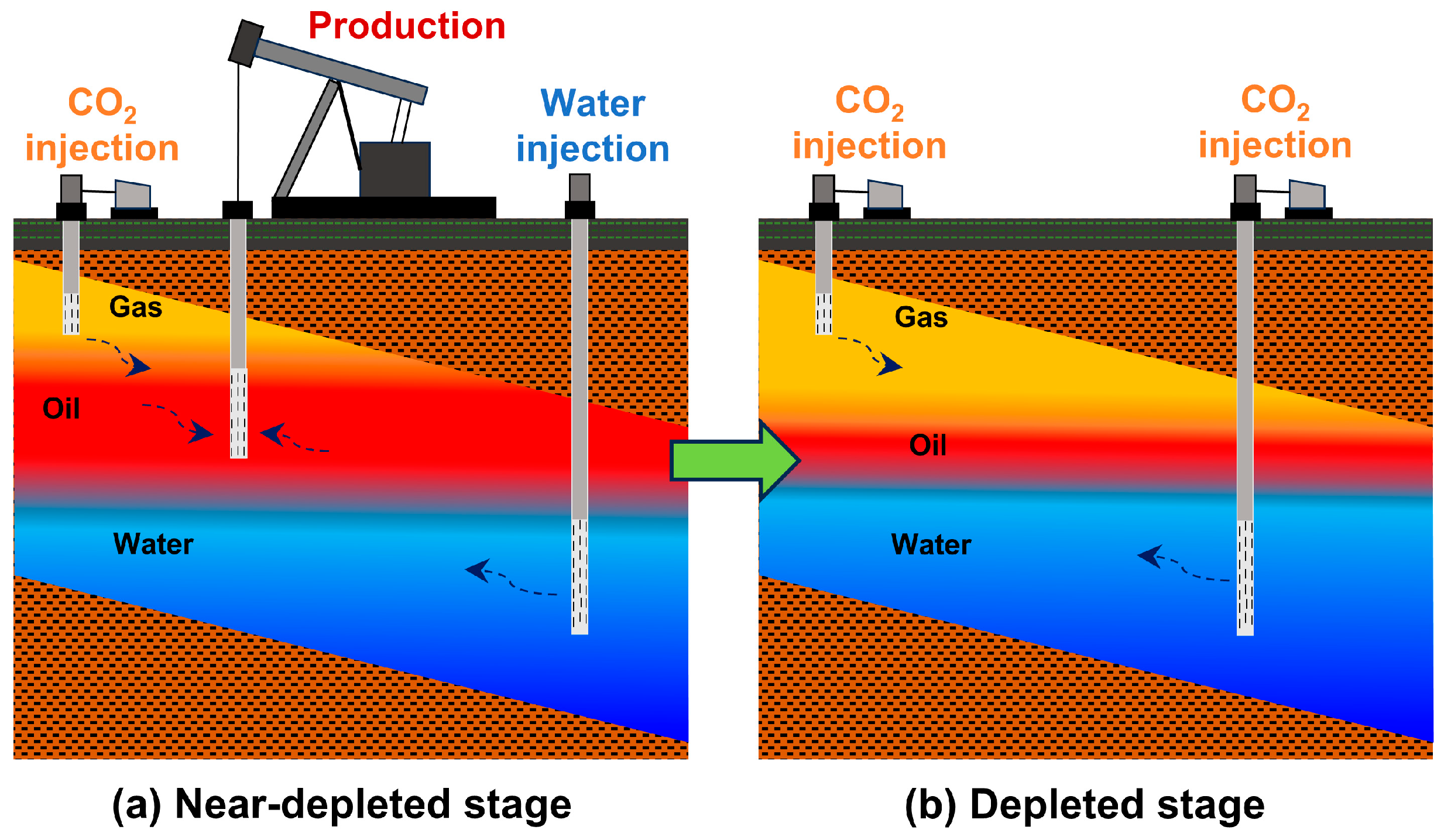
Figure 2.
Distribution of geologic model parameters.
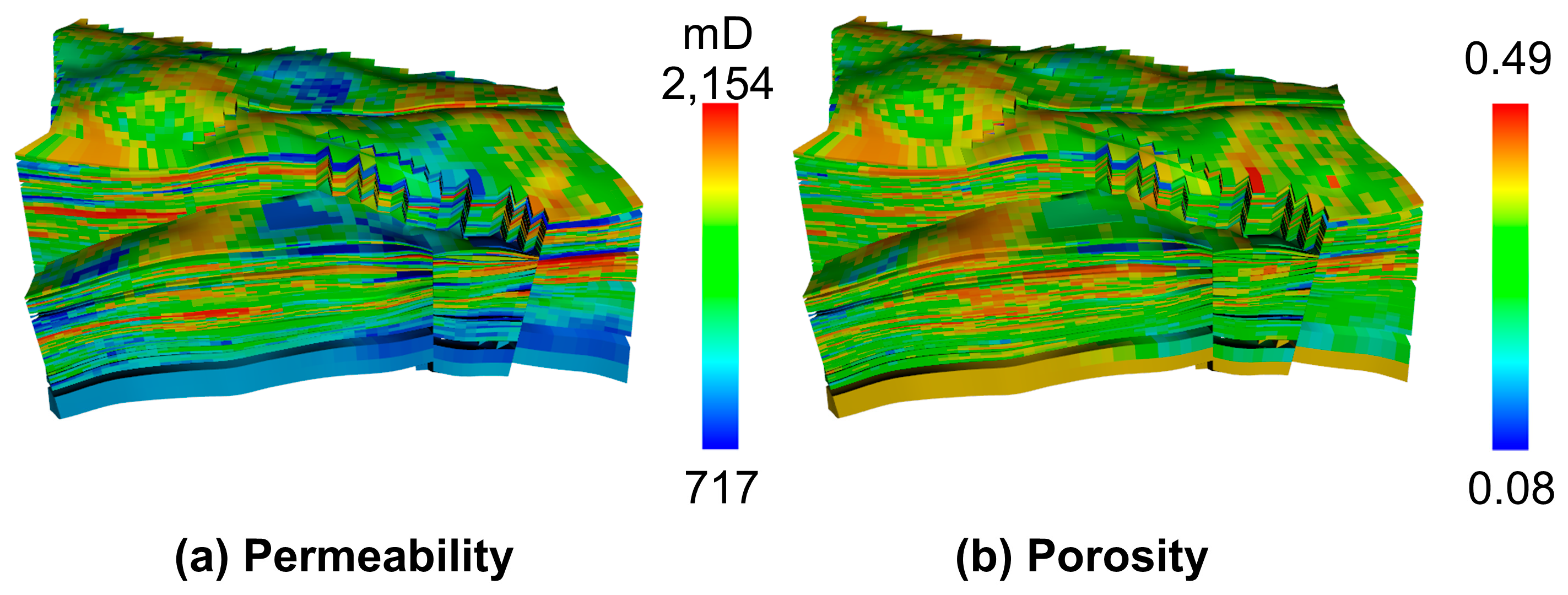
Figure 3.
Distribution of oil at the start and end of the water drive.
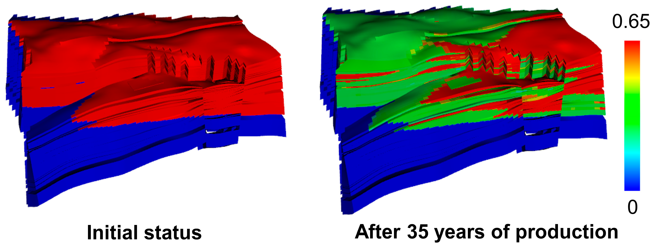
Figure 4.
Cumulative oil production volumes of different injection modes under surface condition for 7 years.
Figure 4.
Cumulative oil production volumes of different injection modes under surface condition for 7 years.
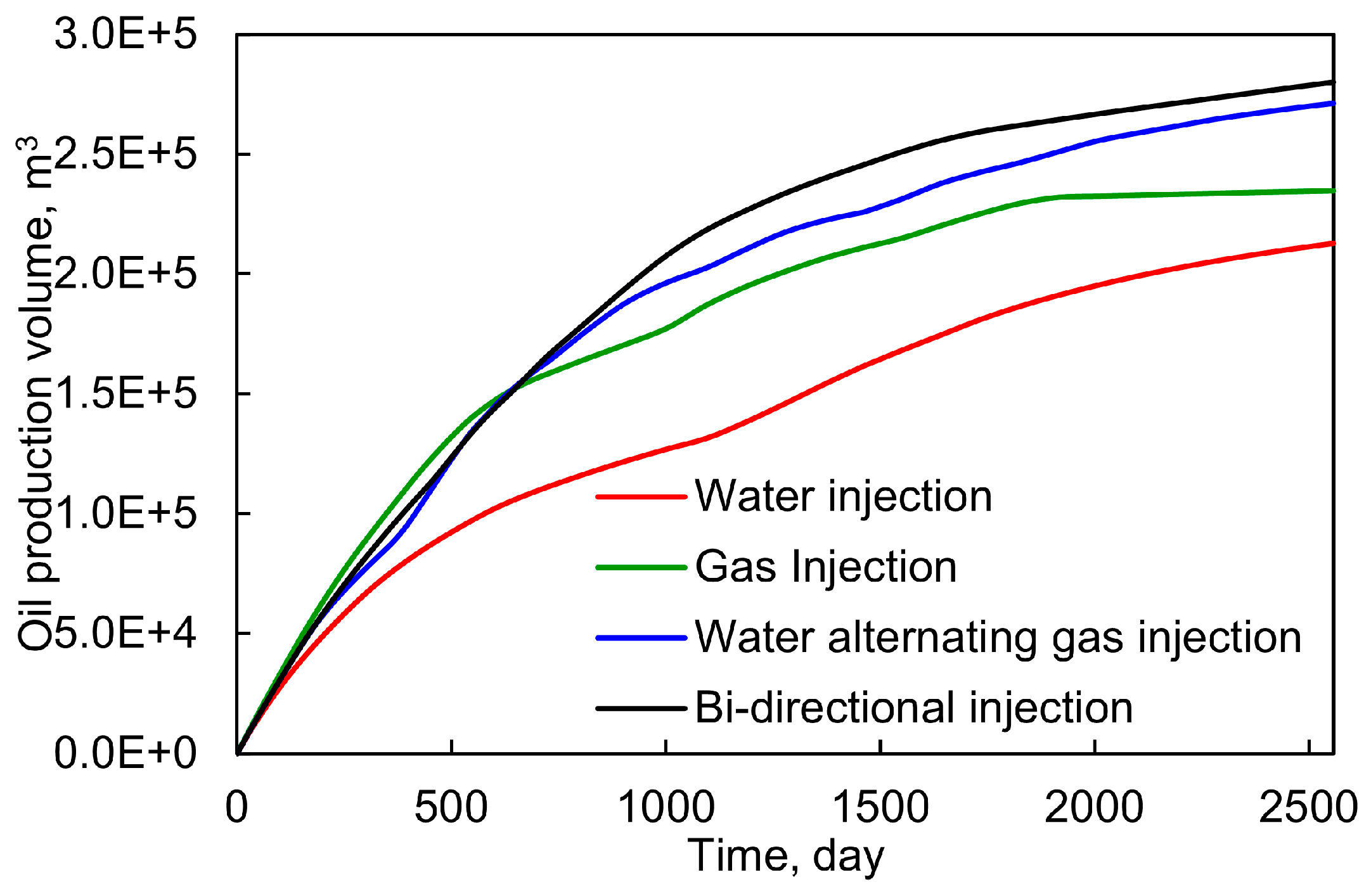
Figure 5.
Oil saturation of the different injection modes after 7 years.
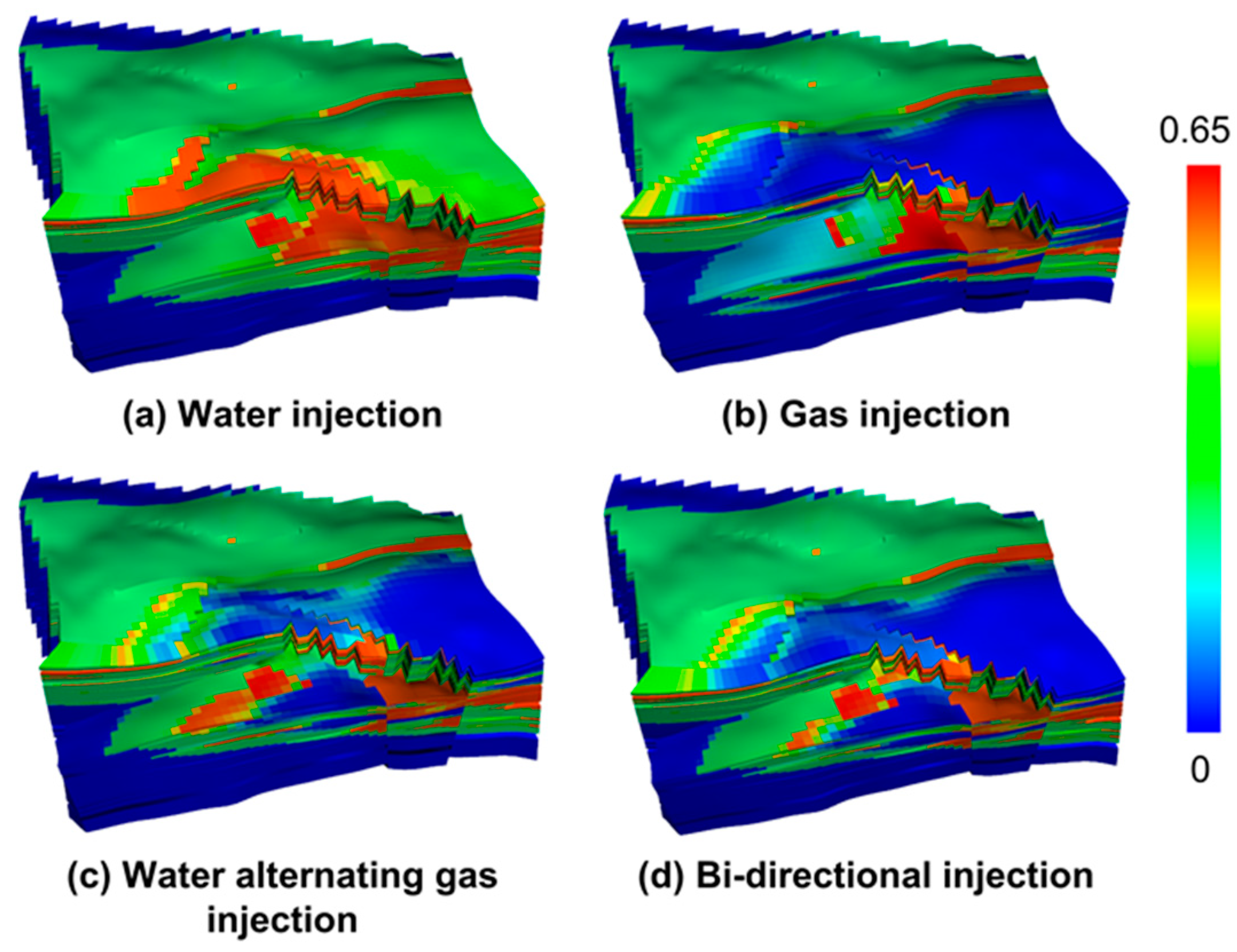
Figure 6.
Injection and production volumes for different injection modes under reservoir conditions after 7 years.
Figure 6.
Injection and production volumes for different injection modes under reservoir conditions after 7 years.
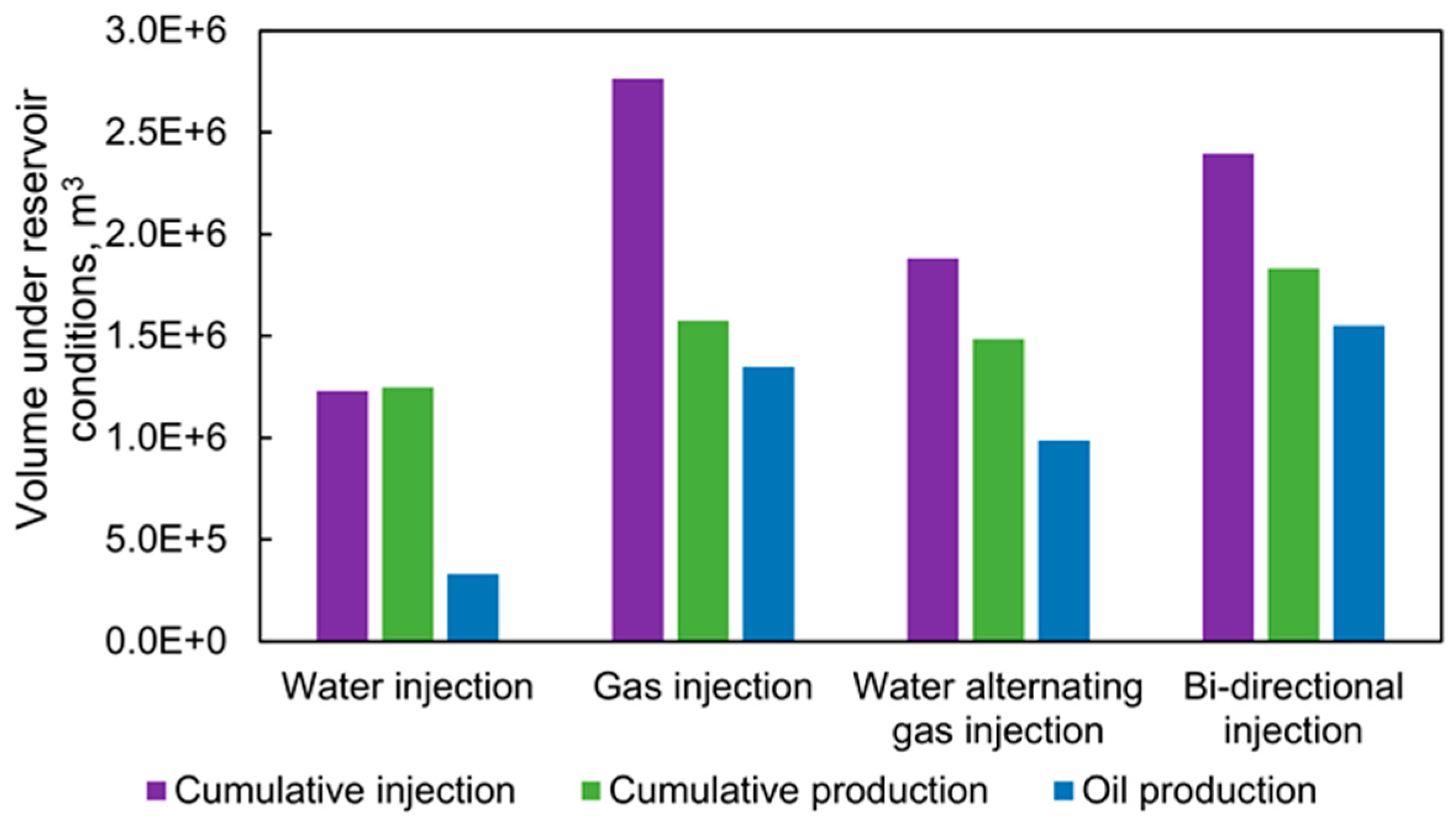
Figure 7.
Cumulative oil production volumes and water cut of different injection pressures for 10 years (— represents Oil production volume; --- represents Water cut).
Figure 7.
Cumulative oil production volumes and water cut of different injection pressures for 10 years (— represents Oil production volume; --- represents Water cut).
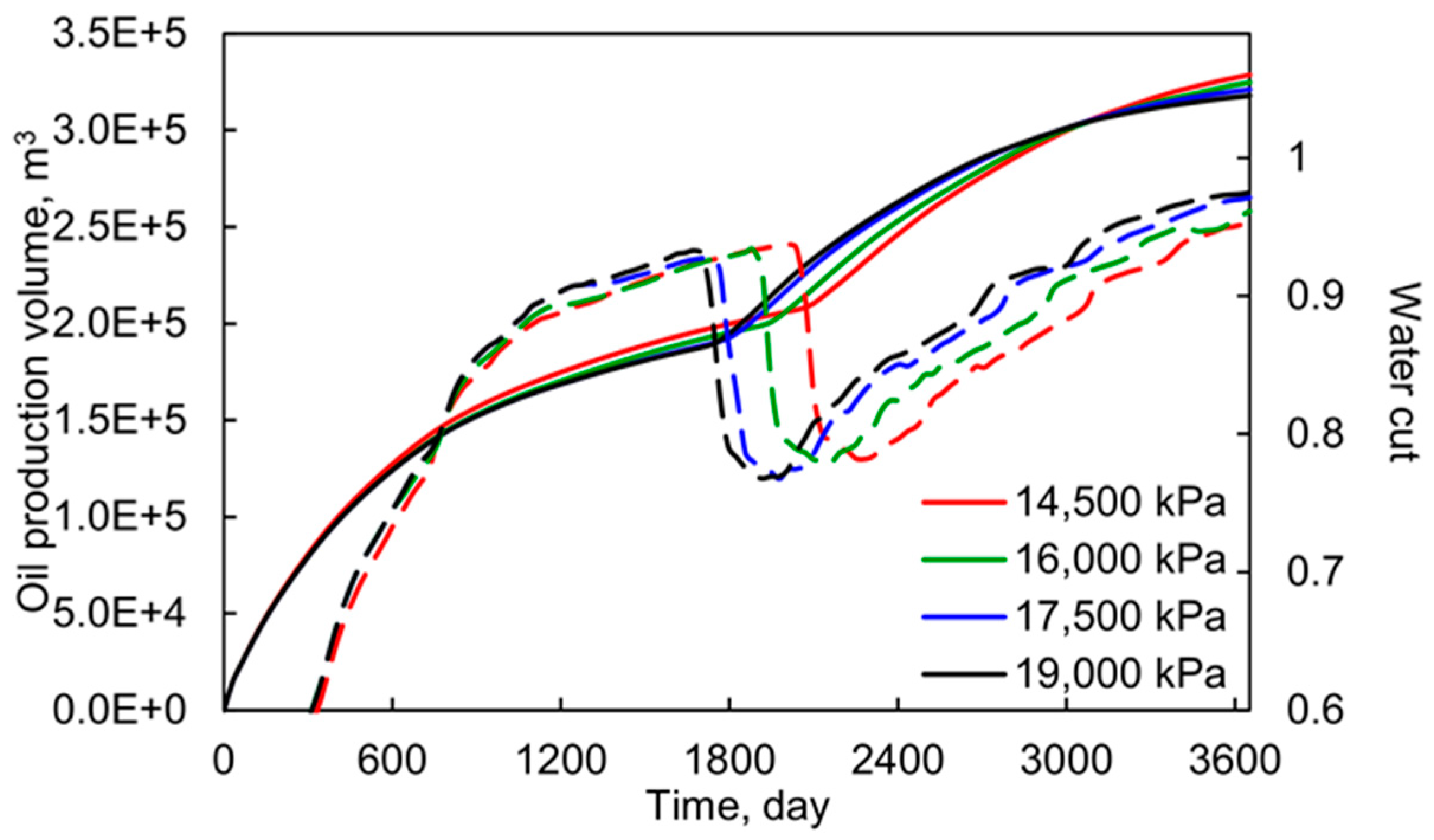
Figure 8.
Gas oil ratio of different injection pressures after 10 years.
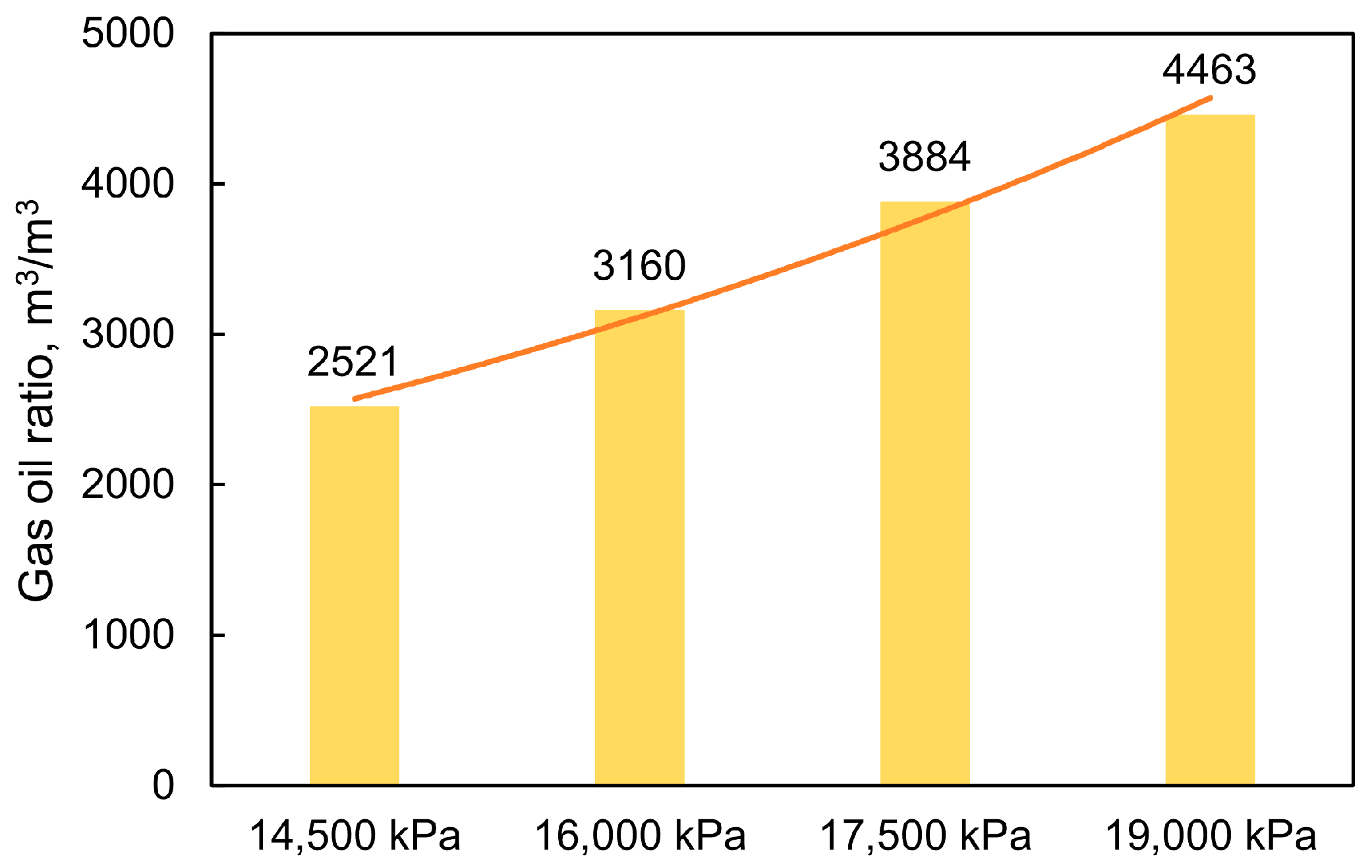
Figure 9.
Cumulative oil production volumes of different gas injection rates for 7 years.
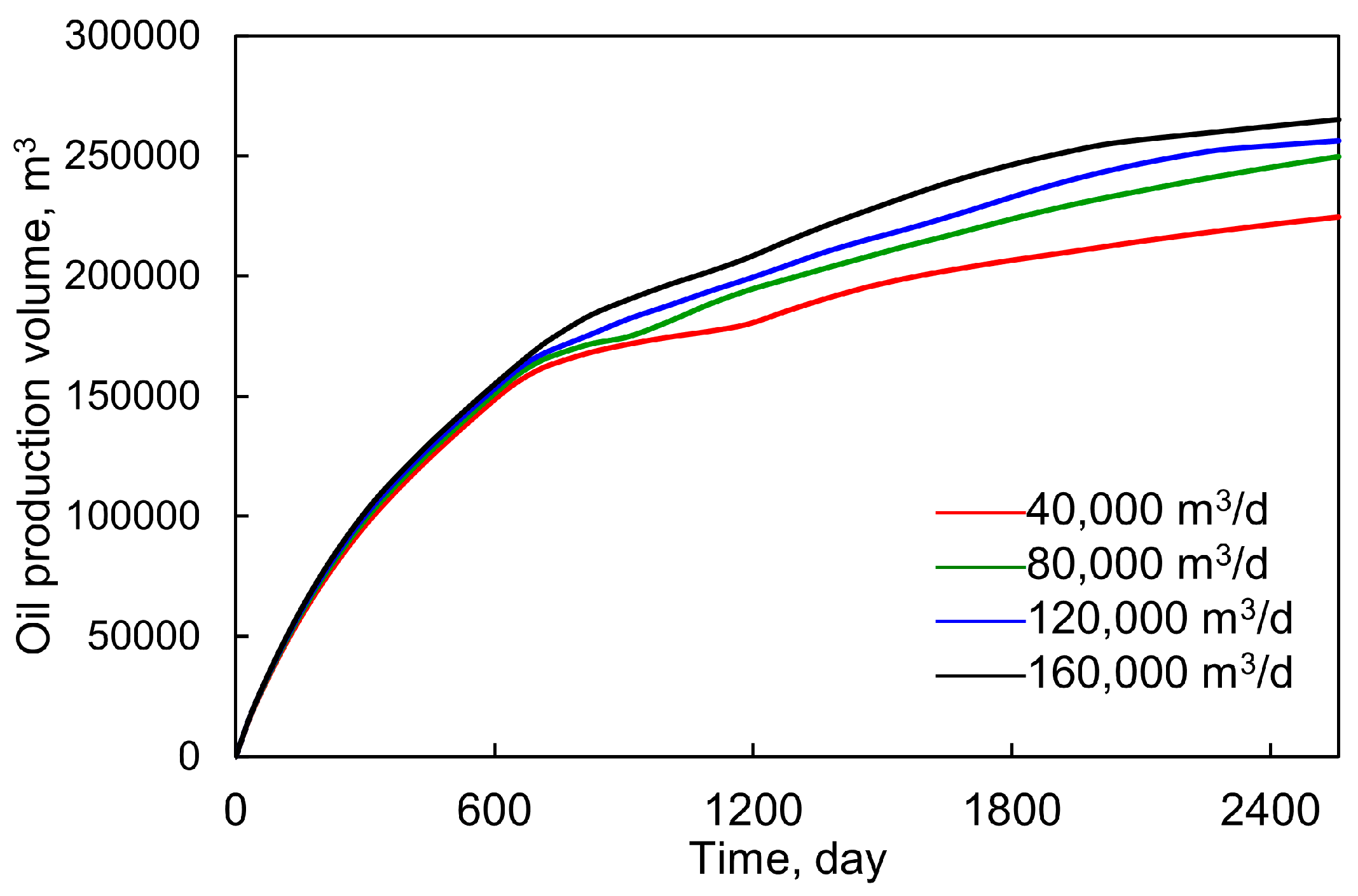
Figure 10.
Gas oil ratio of different gas injection rates after 7 years.
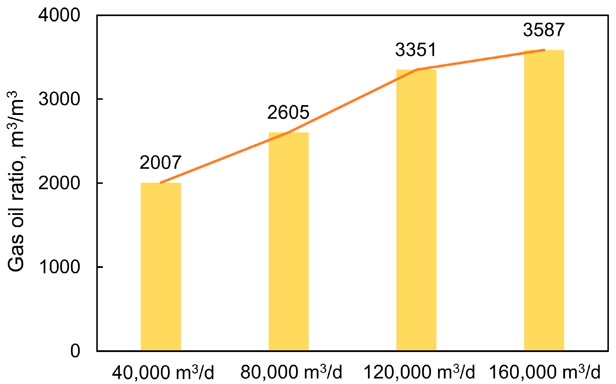
Figure 11.
Cumulative oil production volumes and oil production rates of different liquid production rates for 7 years (— represents Oil production volume; --- represents Oil production rate).
Figure 11.
Cumulative oil production volumes and oil production rates of different liquid production rates for 7 years (— represents Oil production volume; --- represents Oil production rate).
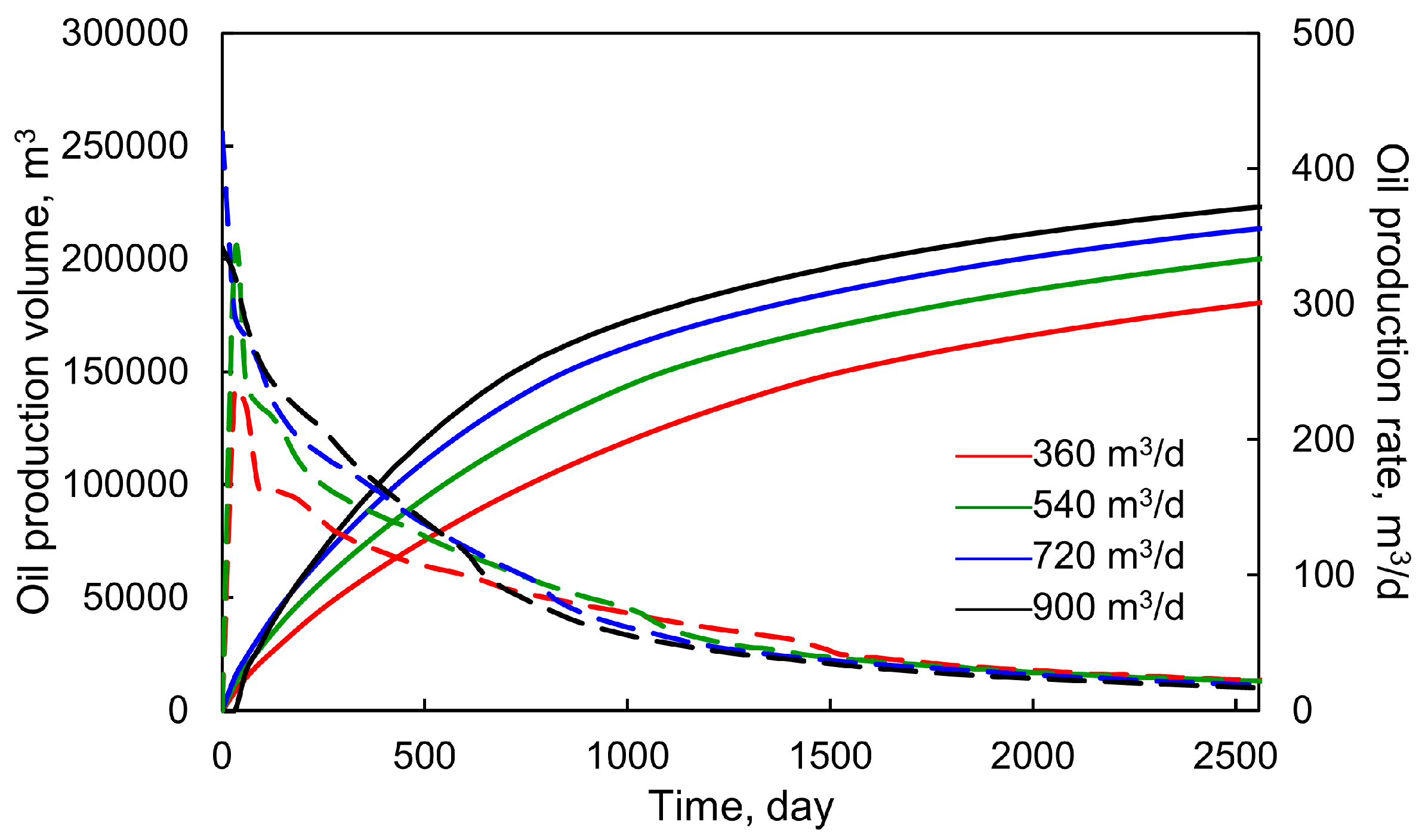
Figure 12.
Gas oil ratio and water cut of different liquid production rates after 7 years.
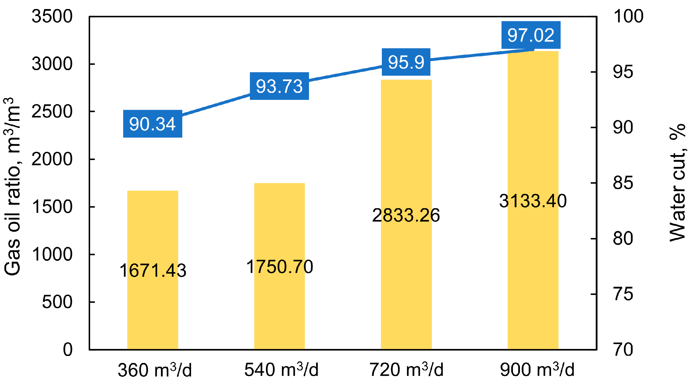
Figure 13.
Distribution of oil and gas after bi-directional injection.
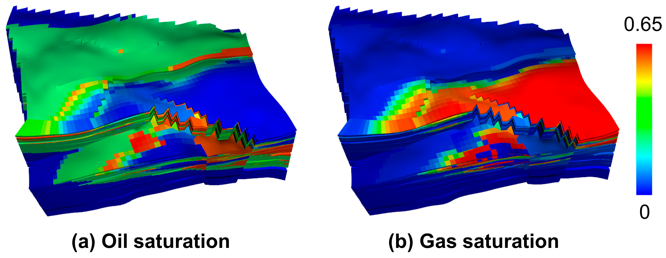
Figure 14.
Cumulative gas storage volumes and gas injection rates of different injection pressures for another 24 years (— represents Gas storage volume; --- represents Gas injection rate).
Figure 14.
Cumulative gas storage volumes and gas injection rates of different injection pressures for another 24 years (— represents Gas storage volume; --- represents Gas injection rate).
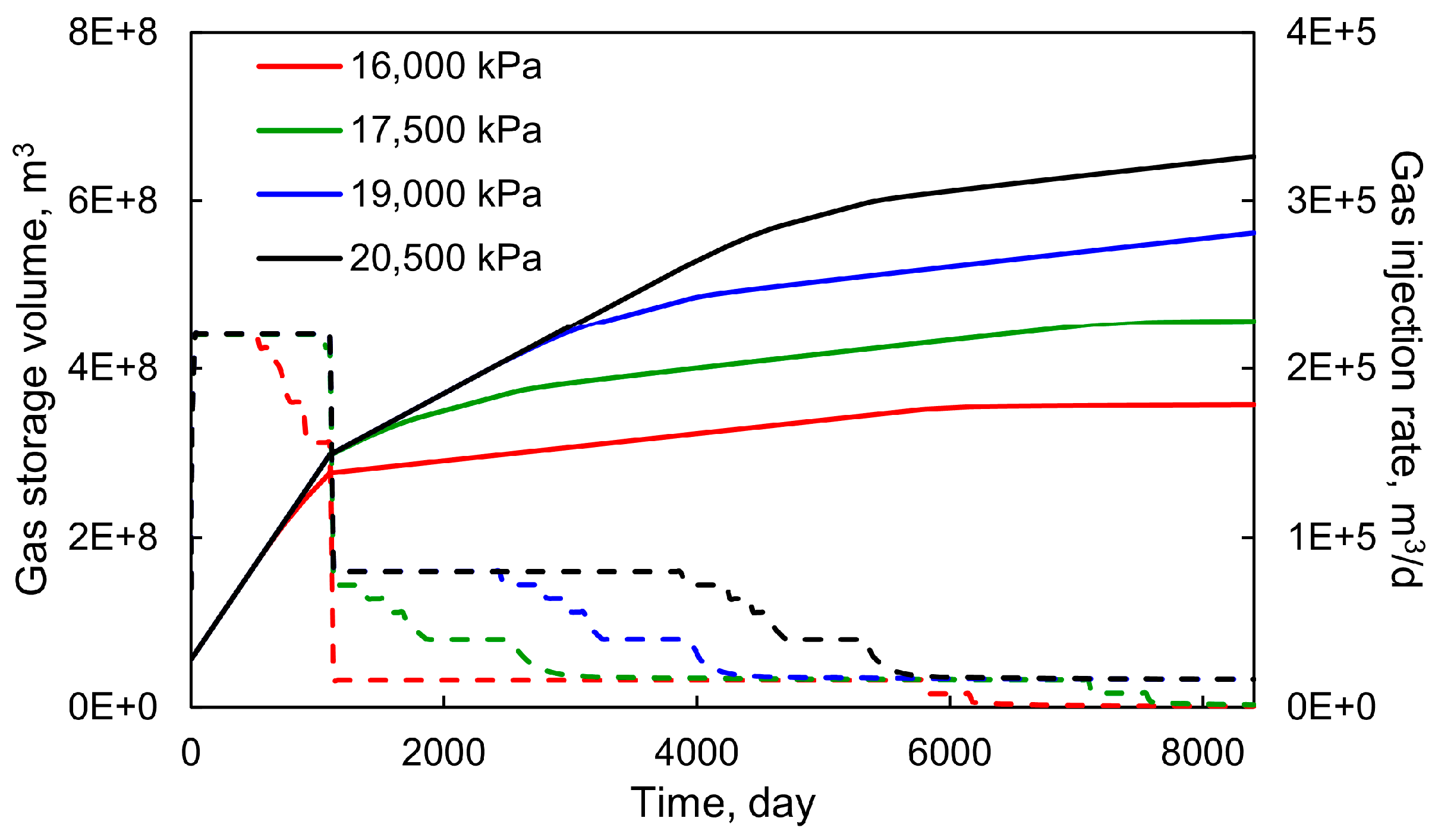
Figure 15.
Gas saturation of the different injection pressures after another 24 years.
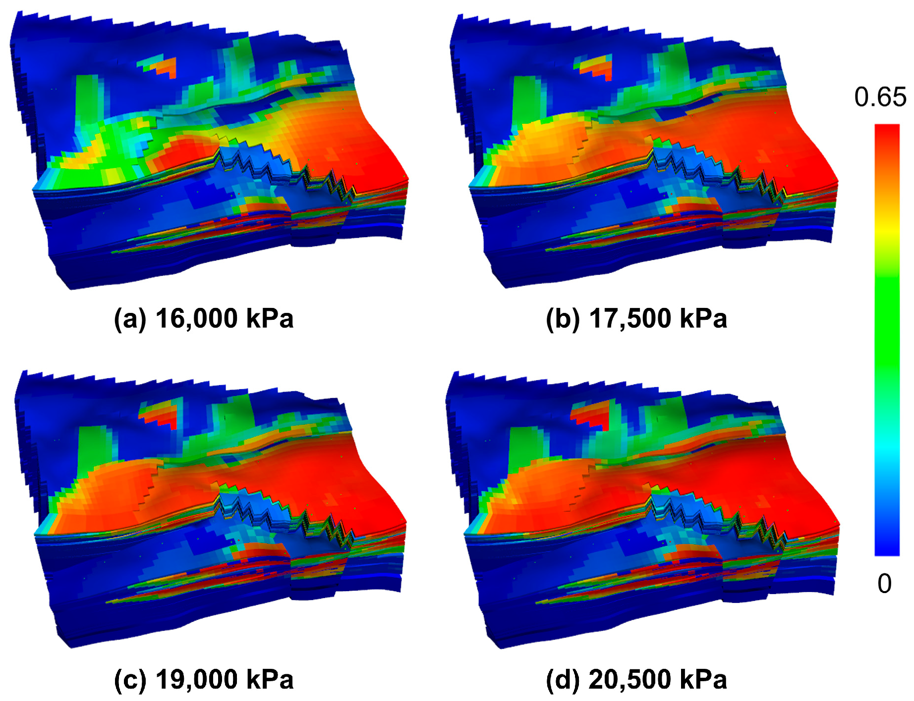
Figure 16.
Cumulative gas storage volumes and gas injection rates of different injection rates for another 24 years (— represents Gas storage volume; --- represents Gas injection rate).
Figure 16.
Cumulative gas storage volumes and gas injection rates of different injection rates for another 24 years (— represents Gas storage volume; --- represents Gas injection rate).
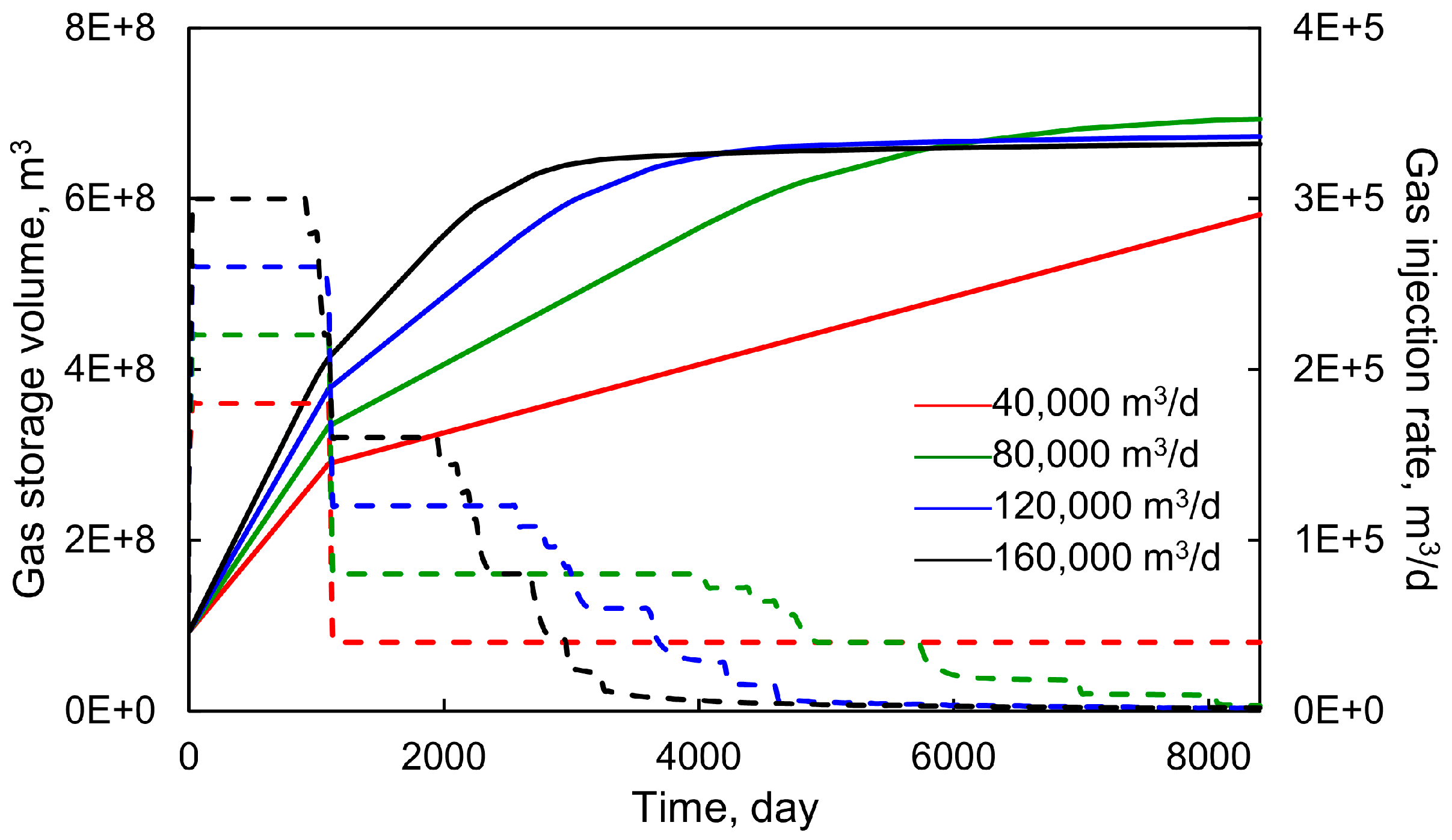
Figure 17.
Gas saturation of the different injection rates after another 24 years.
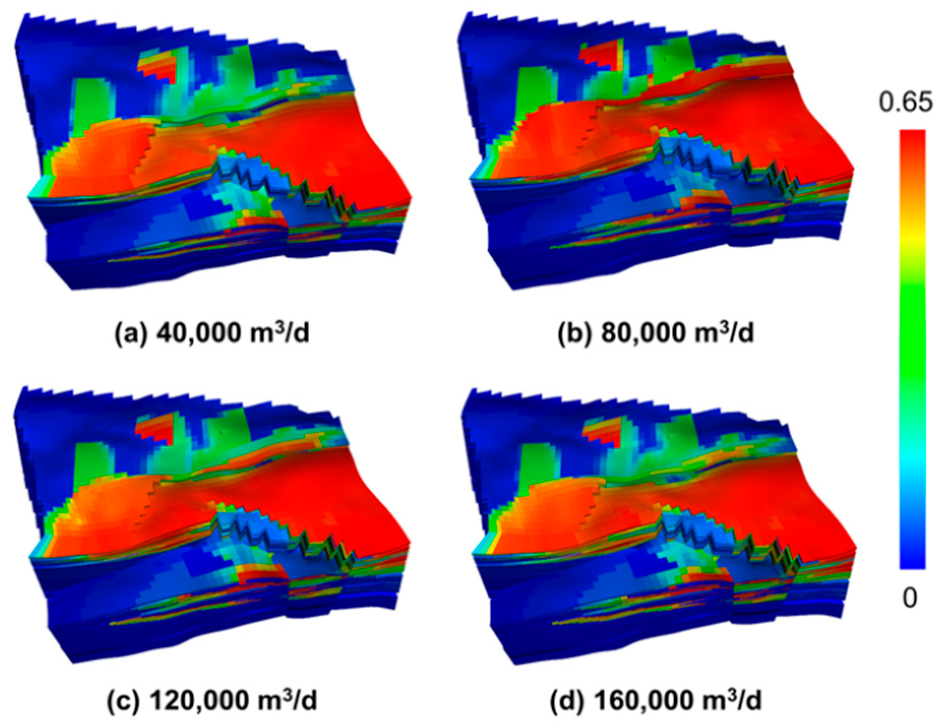
Figure 18.
Cumulative gas storage volumes of intermittent gas injection for another 24 years.
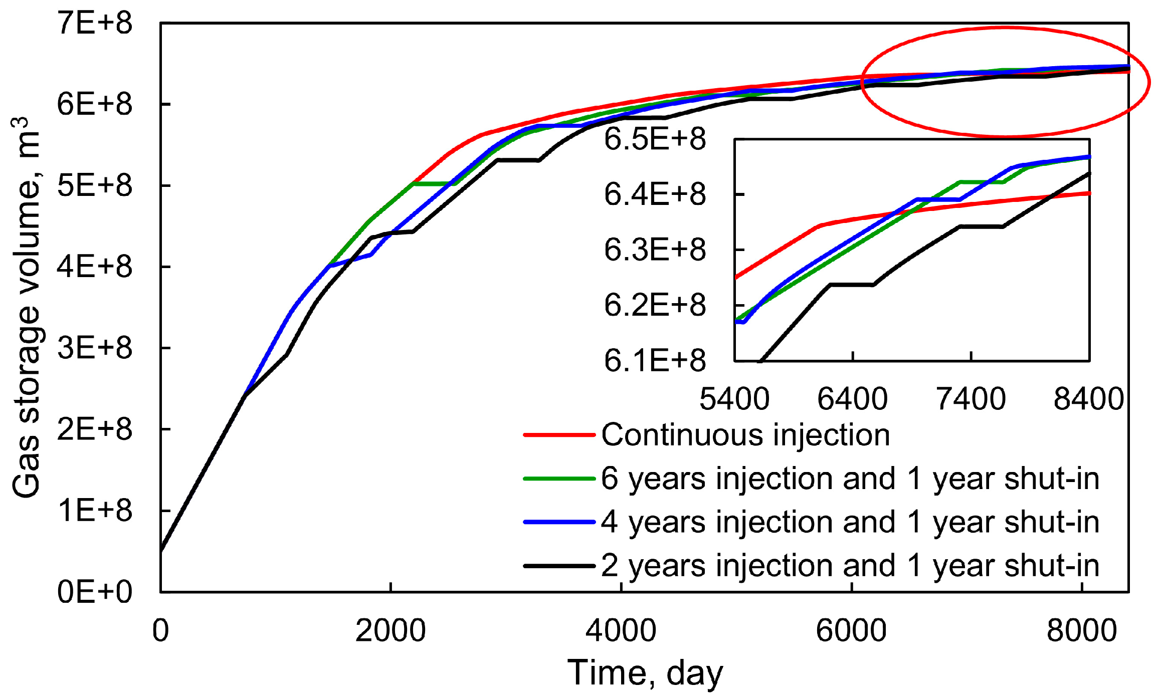
Figure 19.
Percentage and moles of different storage mechanisms for the total 31 years.
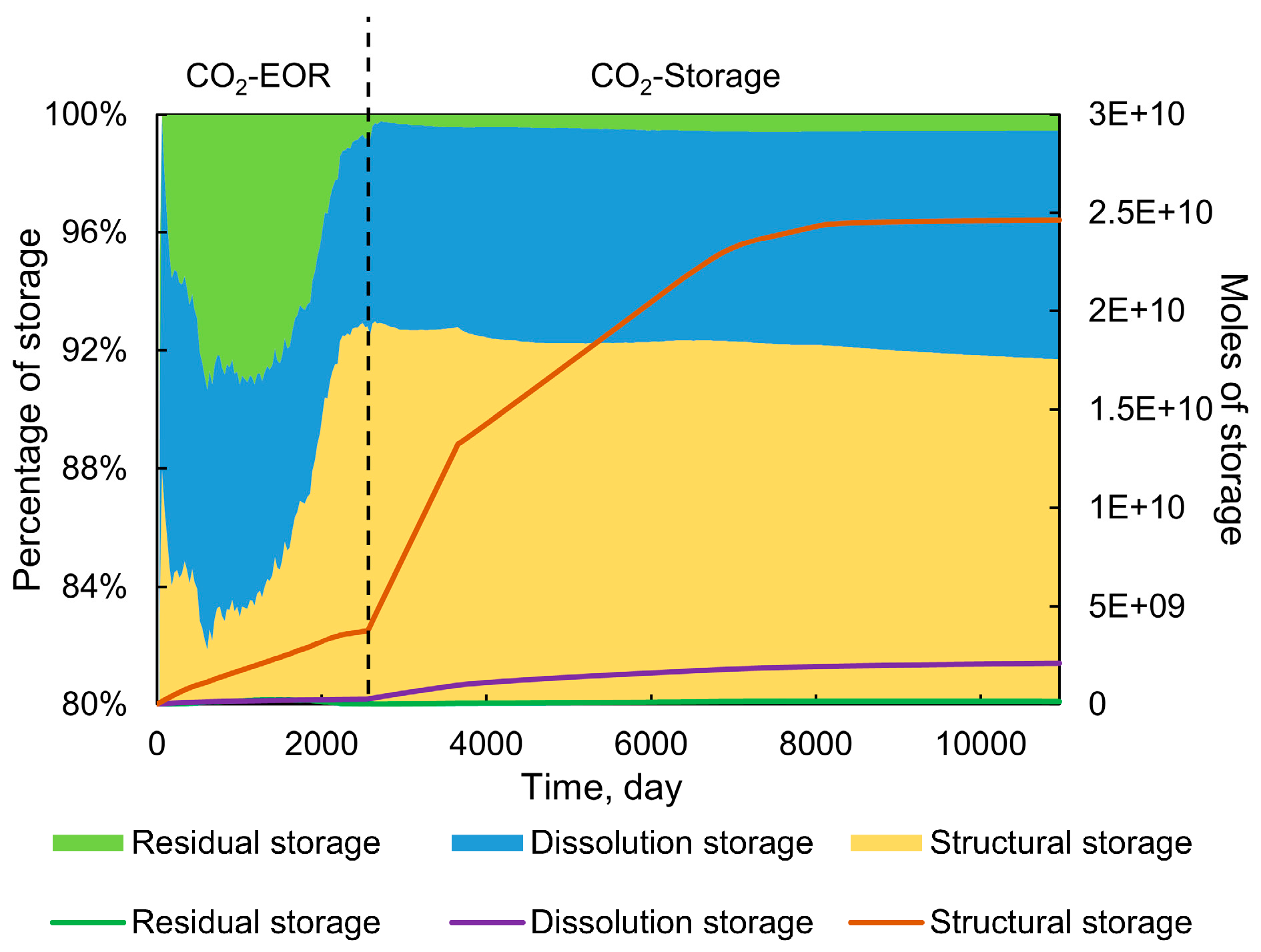

Table 1.
This is a table. Tables should be placed in the main text near to the first time they are cited.
Table 1.
This is a table. Tables should be placed in the main text near to the first time they are cited.
| Septal interlayer | Composition | Mechanisms of formation |
| Muddy | Mudstones, siltstones, muddy siltstones, shales | Sedimentation due to diminished hydrodynamics, with complete sheltering effect. |
| Calcareous | Calcareous siltstones, calcareous mudstones, calcareous shales | Related to the unevenness of the carbonate formation and dissolution, it is found at the junction of the top and base of the sandstone with the mudstone. With complete sheltering effect. |
| Stratigraphy | Sand, mud | Partially sheltered. |
Disclaimer/Publisher’s Note: The statements, opinions and data contained in all publications are solely those of the individual author(s) and contributor(s) and not of MDPI and/or the editor(s). MDPI and/or the editor(s) disclaim responsibility for any injury to people or property resulting from any ideas, methods, instructions or products referred to in the content. |
© 2024 by the authors. Licensee MDPI, Basel, Switzerland. This article is an open access article distributed under the terms and conditions of the Creative Commons Attribution (CC BY) license (http://creativecommons.org/licenses/by/4.0/).
Copyright: This open access article is published under a Creative Commons CC BY 4.0 license, which permit the free download, distribution, and reuse, provided that the author and preprint are cited in any reuse.


