
Submitted:
23 September 2024
Posted:
24 September 2024
You are already at the latest version
Abstract
Aquatic environments are generally heterogeneous in space and time, and the marine organisms have their ways response to those environmental heterogeneities. Cutlassfish (Trichiurus spp.) once is one of the “Chinese Four Major Marine Fish Species” along the coast of northwest Pacific Ocean. There are some comments on the cutlassfish (T. spp.) name identification. In this study, three cutlassfish species, namely, the largehead hairtail (T. japonicas) in East China Sea (ECS), Chinese short-tailed hairtail (T. brevis), and South China Sea (SCS) cutlassfish (T. nanhaiensis), have been identified in the northwest Pacific Ocean. This work integrated 115 studies in cutlassfish population dynamics from 24 sites across 8 countries in the world. The biomass distribution of T. japonicas in the ECS and T. nanhaiensis in SCS, was found to be highly correlated with water temperature and salinity. Spatiotemporal heterogeneity of cutlassfish is found to correlate with both genetic and environmental characteristics in the northwest Pacific Ocean (e.g., density dependency, primary productivity and climate ocean oscillation). Closely related species coexisting in the same shelf region (e.g., T. japonicus and T. nanhaiensis in ESC) often differ in diet and microhabitat. The difference of skull phenology between T. nanhaiens and T. brevis is found to correlate with species separation and environmental heterogeneity. With the implications for the design of ecological research programs on cutlassfish, our study found that the effect of temporal changes outweighs (to some extent) the effect of spatial changes on cutlassfish in those shelf regions.
Keywords:
Trichiurus spp.
; spatiotemporal heterogeneity
; population dynamics
; meta-analysis
; the northwest Pacific Ocean
1. Introduction
Environments are spatially and temporally heterogeneous, and the marine organisms have their ways response to those environmental heterogeneities [1,2]. Temporal heterogeneity shows as variability over time in the extent and quality of habitat, or ecological disturbance [3]. It is important factor to elicit demographic responses, whereas spatial heterogeneity is often related to habitat patchiness [1,4]. For example, the weaker competitors may find a more favorable site or time to spread under environmental stresses. Spatiotemporal heterogeneity in population abundance had been discussed in many studies [3,5,6,7]. Studies on the distribution and diversity patterns of species traditionally have relied on small-scale and local processes [8,9,10,11,12]. In this study, we drive a pattern to quantify the effect in the spatial ecosystem and population dynamics model for cutlassfish (Trichiuridae. spp. Linnaeus 1758) species.
Cutlassfish (T. spp.) (also often referred to as hairtails) is an economically important marine taxa around the world, especially in the China seas [13,14]. The China seas are including the East China Sea (ECS), the South China Sea (SCS), the Yellow Sea (YS) and the Bohai Sea (BH). The scientific name identification and species distribution of the cutlassfish have been summarized in Table 1 [13,15,16,17,18,19]. Based on the complete mitochondrial genome sequence, the improvement name identification has been suggested, namely, the largehead hairtail (T. japonicas) in East China Sea (ECS), Chinese short-tailed hairtail (T. brevis), and South China Sea (SCS) cutlassfish (T. nanhaiensis). The SCS (in Chinese “nanhai”) cutlassfish (T. nanhaiensis, [20]), was often called T. lepturus in some literatures. There are some comments on this species’ name identification. Cutlassfish was reported to thrive in 145 countries (or islands) and is classified as endemic, native, or introduced [13,15,17,21]. Since their similarity in morphology and their overlap in distribution, the samples from the normal surveys were often not identified to the species level. In SCS, T. nanhaiensis is mostly commonly observed, with a small fraction of T. japonicas and T. brevis, whereas in the YS, BH, and southern seas of Japan/East Sea (SOJ), the T. japonicas is mostly commonly observed [14]. In the ECS, T. japonicas is mostly common, with a small fraction of T. brevis and is one of the most economically important fish species in the northwest Pacific Ocean [20,22] (Figure 1). According statistics from Japanese fishery, T. japonicus is widely distributed offshore in the Sea of Japan (SOJ) around Kyushu [15]. In the seas of Japan/East Sea, cutlassfish (T. spp.) is commonly called ribbon fishes or “tachi-uo” (in Japanese) [17]. T. japonicas is a widely distributed coastal species that thrives throughout the tropical and temperate waters of the world between the latitudes 60° N and 45° S, including all China seas [23]. Coastal China seas are rich with high levels of terrigenous nutrients coming from the Asian continent through river runoff, which has led to high primary productivity and increased fish production [12,24].
Previous work on the cutlassfish focused on the growth of individual or reproduction of population [15,16,22]. Cutlassfish are voracious predators and prey on pelagic and benthic species, such as small fish, zooplanktonic and benthic crustaceans, and cephalopods [17,25,26,27]. The spatial and temporal distribution of fish feeding habits should been changed with the regional and seasonal variations [28]. Comparison of the cutlassfish spatiotemporal heterogeneity in population dynamics and explaining these variations based on the regional oceanographic conditions are largely lacking [29,30]. The seasonal variation was studied in the feeding habits of T. japonicas in the ECS [31]. A spatial ecosystem and population dynamics model (SEAPODYM) and metapopulation models were used to address the temporal variation in population growth rates caused by changes in species composition [29,32,33,34]. SEAPODYM had been used to describe spatial dynamics of many species, such as tuna and tuna-like species [29,30]. Oceans serve as the earth’s dominant reservoirs of heat, carbon, and energy, and are in near equilibrium with the atmosphere, lithosphere, and biosphere [27,35]. Meta-analysis is often used as an appropriate method for combining evidence from numerous trials and quantifying homogeneity and heterogeneity among these studies [36,37,38,39].
Our study aims to evaluate the dynamic responses of cutlassfish to environmental variation, which will be a challenge because of limited data. More than 100 studies on cutlassfish from 24 sites across 8 countries were compiled in this study, including all China seas and the Sea of Japan. Research history, management foundation and environmental facts will be reviewed in this study, and the meta-analysis method will be used to assess the spatiotemporal features of the population dynamics. The effect of temporal (i.e., maturity age, spawning time, and lifespan) and spatial (i.e., species dispersal distance, longitude, latitude, size, and sea level) factors of the life history of cutlassfish was tested through a meta-analysis of variance. The information will take important implications for the management/conservation of this species in the northwest Pacific Ocean.
Our study aims to evaluate the dynamic responses of cutlassfish to environmental variation, whereas it will be a challenge because of limited data. Here about 115 studies on cutlassfish from 24 sites across 8 countries were compiled in this study, including all China seas and the Sea of Japan. Research history, management foundation and environmental facts have been reviewed in this study. The effect of temporal (i.e., maturity age, spawning time, and lifespan) and spatial (i.e., species dispersal distance, longitude, latitude, size, and sea level) factors of the life history of cutlassfish was tested through a meta-analysis of variance. The information will take important implications for the management/conservation of this species in the northwest Pacific Ocean.
2. Materials and Methods
2.1. Data Collection and Materials
Life history and ecology traits of the T. japonicas, T. nanhaiensis and T. brevis were reported in the published literatures [14,31,40,41,42]. Biotic factors contain the chlorophyll A concentration (the primary productivity of the ecosystem, available from Ocean Color Web). The fishery data and abundance were extracted from the most recent stock assessment reports. Global climate indices, such as Pacific Decadal Oscillation (PDO), were obtained from National Oceanic and Atmospheric Administration. The natural mortality (M), fishing mortality (F) and exploitation ratio (E) of cutlassfish (T. spp.) were obtained from the Chinese-Norwegian “BeiDou” project survey from the bottom trawl fisheries in the China Seas. The growth information of the cutlassfish (T. spp.) has been summarized in Table 2. The age–at–maturity of cutlassfish is 1–2 years, and the anal length of species is approximately 50-60 cm [14,22]. The total length of cutlassfish can exceed 200 cm, and it can live for more than 15 years [42]. The catch and effort data of cutlassfish (T. spp.) in the China Seas are from the Compilation of the statistics of Chinese fishery (1984-2012) (in Chinese). The variability of the cutlassfish (T. spp.) catches and the percentage of the total fish production (from all the seas in China) are from the Compilation of the statistics of Chinese fishery (1950 to 2011).
2.2. Modelling Growth Parameters and Population Variability
The dynamic states are based on the production model, which is one of the simplest model-based methods for estimating maximum sustainable yield, such as the Schaefer model (1954) [43]. New simple method (catch-based model) uses catch data plus readily available additional information to approximate maximum sustainable yield with error margins, and this set of viable r–k combinations can be used to approximate maximum sustainable yield for a given stock [44].
where W∞ is the von Bertalanffy growth parameter, k is the carrying capacity, and r is the maximum rate of population increase, and the ranges for the random samples of r could be acquired from the resilience assignment in FishBase [44]. Original single-species meta-population model is one of the fundamental ways in which nutrient support is linked to the growth rates of phytoplankton [29,32,45]. The nutrients across the base of the euphotic layer are thus balanced by the phytoplankton uptake integrated over the euphotic depth, which is given by [12,30],
where p(t) denotes the proportion of the occupied spatial ecosystem at time t, c is the colonization rate of the empty ecosystem; e is the extinction rate of the occupied ecosystem; μ is an uptake rate for the nutrient (depends on the growth rate of the phytoplankton); <ωc’>zeu is the vertical supply rate of nutrients; w is the vertical component of the velocity; and zeu denotes the euphotic depth.
2.3. Modelling Feeding and Spawning Migration
Migrations of feeding and spawning are often observed because of their life history and/or prey availability. SEAPODYM that includes feeding habitat index (FHI), spawning habitat index (SHI), and spawning and feeding migration index (SFMI) can be written as,
where Φa,n denotes an accessibility coefficient calculated for each forage (F) component; Φ0(to) is the spawning temperature index; Ψn is the dissolved oxygen content; Oz is the dissolved oxygen concentration in layer z; is the oxygen value for Ψ=0.5; γ is a curvature coefficient. Multiple factors influence the distribution of cutlassfish species distribution. Λ is the ratio between food abundance and predator density; Κ is a curvature parameter; Gd is the day-length gradient; is the threshold in the day-length gradient at which the switch occurs; and Iα is the fish size at age a.
2.4. Estimating Temporal Heterogeneity and Identifying driving Factors
The temporal heterogeneity of cutlassfish growth is derived from the changes of the marginal growth index (MGI) variability over time; and the average predictive differences (APD) was used to describe how the response variable (e.g., MGI) varies as other potential driving variables change [14,30]:
where is the estimated otolith radius (R) at PLt (preanal length at age t) calculated using equation , and rmax is the estimated size of the outermost annulus [17,37].
2.4. Meta-Analysis
3. Results and Discussion
3.1. Main Marine Ecosystems (i.e. Region 1, Region 2, Region 3 and Region 4)
In the northwest Pacific Ocean, to reveal the regional population dynamics responses of those cutlassfish species to different oceanographic conditions, the data set was divided into different groups corresponding to the four main marine ecosystems (i.e. Region 1, Region 2, Region 3 and Region 4).
3.2. Seas of Japan/East Sea (T. japonicus)
Based on Japanese fishery statistics, T. japonicus is widely distributed offshore in the Sea of Japan (SOJ) around Kyushu. The spatial-temporal heterogeneity of cutlassfish was determined from the changes of the MGI variability from April to December in the SOJ. The average predictive difference of MGI for cutlassfish in the SOJ on the variability spatial scale (i.e. distance to land: coastal < 20m, inner shelf 20–80m, outer shelf 80–120m, and Shelf break 120–350m) was compared with temporal changes from April to December (Figure 2). The average annual landing was 225 tons (from 1983 to 1993) with a maximum of 685 tons (1984). The preanal length (PL) of T. japonicas ranges from 17.2 cm to 44.7 cm in Kagoshima Bay, southern Japan (Shih, 2004). Previous studies divided the stocks of T. japonicas into two or three cohorts in relation to the spawning season in the SOJ, and considered that early sexual maturation would cause the growth rate decrease.
3.3. Yellow Sea and Bohai Sea (T. japonicas)
Based on statistics from Chinese fishery (1984–2012), the data set was divided into different groups corresponding to the three main marine ecosystems (i.e. Region 2, Region 3 and Region 4). The YS and BH share a wide and shallow continental shelf with the ECS. In the YS, the first record of fishery of T. japonicas was in Zhucheng, Shandong Province, which was established during the Qing Dynasty (A.D. 1644–1912), while other fisheries spun off in other parts of the Shandong Province, such as Laiyang and Muping, during 1950s (the People’s Republic of China Period). The T. japonicus catch sharply declined in the BH and YS during the 1960s, which was earlier than the decline in ECS, and was attributed to overfishing. After 1995, T. japonicus in this region has been harvested only as bycatch of other target fisheries.
3.4. East China Sea (T. japonicas and T. nanhaiens)
T. japonicas is found throughout Chinese coastal waters whereas T. nanhaiens is distributed from the SCS to the southern part of the ECS. Cuttlefish (Sepia officinalis), small yellow croaker (Larimichthys polyactis), large yellow croaker (Pseudosciaena crocea) and cutlassfish (specially the T. japonicas) were once “Chinese Four Major Marine Fish Species” [46]. Currently, the large yellow croaker is already endangered, and although the cutlassfish population has declined significantly, it is still considered as the most caught fish species among the four species [46]. For the T. japonicas, the difference of the estimated population sizes between T. japonicus (ECS) and T. japonicus (YS and BH) reaches an order of magnitude, suggesting that the ECS is approximately 10 times more than conducive for the population growth of T. japonicus compared with the other three China Seas. The changes of the catch variability and demographic history of T. japonicas in the ESC, BH, and YS have been assessed using the mitochondrial cytochrome b sequences. Growth parameters, such as intrinsic growth rate (r), maximum sustainable yield (MSY) and carrying capacity (k), with their relations to catch variability were estimated by the Catch–MSY for T. japonicas in the ECS (Figure 3). The response to environmental changes of cutlassfish in the ECS is related to both fishing pressure and climate variability, and the fluctuations in food supply drive recruitment variation in this species [43,47,48]. The versions of SEAPODYM and metapopulation model include the expanded definitions of habitat indices, movements, and natural mortality based on empirical evidences [30]. SEAPODYM showing different biological characteristics of T. japonicas, T. brevis and T. nanhaiensis in ECS is presented to illustrate the capacity of the model to capture many important features of spatial dynamics of cutlassfish. SFMI of T. japonicas separated in summer and winter is found to correlate with different sizes (i.e., preanal lengths (mm): 80–200, 201–280, 281–400, and > 400) (Figure 4). Given that population size is closely correlated to primary productivity, the carrying capacities and levels of primary productivity between the ECS and “BH and YS” were comparable. Population size increased with increasing temporal scale and decreased with increasing spatial scale. The population growth rates of T. japonicas have declined as human population density increased from 1995 to 2000, which is consistent with density-dependent feedback to survival. Geographical distribution patterns and relationships with temperature, salinity, chlorophyll a, and zooplankton abundance indicated that the T. japonicas population in the ECS spawns in the warm Kuroshio Current and in the zone where the warm Kuroshio Current mixed with the ECS shelf water [49,50].
3.5. South China Sea (T. nanhaiens and T. brevis)
Two species of cutlassfish, T. nanhaiens and T. brevis, constitute the largest proportion (approximately 80%) of the commercial catches of cutlassfish in the SCS [51]. However, the fishery and population status of cutlassfish stocks in the SCS remain unclear [52]. The two species are partially sympatric in the Beibu Gulf (in the northwest SCS) and has been suggested to be distinguished based on their skull and vertebrae phenotypes (i.e., T. nanhaiens has tight frontal bone, whereas T. brevis has loose frontal bone) [14]. Main categories of prey groups and regional feeding distributions of the cutlassfish have been summarized in Table 3. Closely related species coexisting in same shelf region (e.g., T. japonicus and T. nanhaiensis in ESC) often differ in diet and microhabitat. While the difference of skull phenotypes between T. nanhaiens and T. brevis, might be influenced by species separation and environmental heterogeneity in the northwest SCS. In coastal waters of Chinese Taiwan, cutlassfish commonly preys on Benthosema pterotum and Acetes intermedius in the daytime and on Bregmaceros lanceolatus, Benthosema pterotum, and Encrasicholina heteroloba in the nighttime [53].
3.6. Distributions, Prey Groups, and Spatiotemporal Heterogeneity
In the regions (1, 2, 3, and 4), the spatial distribution of the feeding grounds of T. japonicas, T. nanhaiensis and T. brevis are an important factor in determining their prey composition. Regional feeding distributions of T. japonicas, T. nanhaiensis and T. brevis have been summarized in Table 3. Based on the studying the spatial and temporal distribution of fish feeding habits, those species have been shown that their feeding habits are changed with the regional variation, seasonal variations, diurnal variation and ontogenetic. Correlation analysis between cutlassfish catches and environmental factors had implied the spatial heterogeneity in population dynamics (Table 4). The biomass distributions of cutlassfish were found to be correlated with ecological and environmental variations in temperature, salinity, sea level, dissolved oxygen concentration, and primary productions [54]. In the SCS, the tropical cyclones are the major factor affecting fish population, whereas in the ECS, the local runoff and monsoon drive the nutrient distribution directly responsible for the long-term variation of fish population. This study found that the mean sea level trends could be the environmental factor most comprehensively associated with primary productivity distributions (Figure 5).
Regions (1, 2, 3, and 4) have different fish communities associated with different environmental variables (e.g. temperature, salinity, transparency, and depth) and different abiotic characteristics in the northwest Pacific Ocean [55]. Catches variability and demographic history of cutlassfish (T. spp.) have responded the change over time. Effective population size of T. japonicus, including geographic groups from ESC, BH and YS the catches variability and demographic history of T. japonicus have responded the change over time using the mitochondrial cytochrome b sequences (Figure 6). During the Qing Dynasty (A.D. 1644–1912), the coastal regions were closed to fishing because of military concerns, which possibly explains why the effective population size of T. japonicas remained stable during this time [56].
Using the SEAPODYM model, the dependency population dynamics of the three cutlassfish species was accounted for from summer to winter and between five spatial scales (i.e., SOJ, ECS, SCS, YS, and BH). Means, 80% confidence intervals of the distributions of water temperature, salinity, depth and distance to land were perfected to the cutlassfish habitation in the northwest Pacific Ocean, including ECS, SCS, YS, BH, and Seas of Japan/East Sea (Figure 7). Data are from FishBase, and separated by season scale (i.e., summer and winter). Water temperatures and salinity strongly influence cutlassfish biology, abundance and habitat, and temporal-spatial distribution.
The adult cutlassfish feed on epipelagic (0–100 m) or mesopelagic (100–400 m) organisms in daytime and migrate into the bathypelagic layer (400–1000m) at night [50]. Phytoplanktons affect nutrient uptake in a somewhat non intuitive manner [12]. The observed population dynamics differences among cutlassfish species in the seas along the Chinese coast may reflect the responses of cutlassfish to the differences in the changes of regional primary productivity. Three vertical layers, namely, epipelagic (0–100 m), mesopelagic (100–400m), and bathypelagic (400–1000m), are described in published literature [30,34]. Biomass(gm-2) of epipelagic and mesopelagic mid-trophic functional groups (i.e., prey) in the Pacific Ocean (including Seas in China and Seas of Japan/East Sea) daytime have been illustrated (Figure 8). Approximately two-third of cutlassfish diet are epipelagic group (0–100 m), and migrant mesopelagic groups (e.g. Decapterus maruadsi), which are abundant organisms between sunset and sunrise.
3.7. Coupling Phytoplankton Production and Physical Transport
Both the anthropogenic and natural causes for the species distribution patterns in the ocean should both be considered [7,57]. The interactions, including mixing, diffusion, and intrusion, in the Yangtze River and Huaihe River produce the complicated hydrographic conditions of the ECS [28,31]. Information on T. japonicas in BH and YS, such as spawning and feeding grounds, obtained from the local aquatic archives and history records in the Ming (A.D. 1386–1644) and Qing Dynasties (A.D. 1644–1912) are fully consistent with the modern fishery surveys [56,58]. The variability of the total catches of cutlassfish and the proportion accounted for total fish production in the China Sea (i.e. SCS, ECS, YS, and BH) is a response to changes in sea conditions from 1950 to 2011. SEAPODYM model includes a forage (prey) submodel describing the transfer of energy of stored biomass through functional groups of midtrophic levels and an age-structured population submodel of the predator species and their multifisheries [30]. Nutrients across the base of the euphotic layer are thus balanced by the phytoplankton uptake integrated over the euphotic depth [29,32]. Phytoplankton uptake is one of the fundamental ways in which the physical delivery of nutrients affects linked to the growth rates of phytoplankton [12]. The existence and stability of equilibriums depend on the extinction threshold condition and metapopulation dynamics [29]. For the T. japonicas in the ECS and T. nanhaiensis in SCS, the spatiotemporal heterogeneity in population dynamics were found to be correlated with ecological and environmental variations in water temperature, salinity, depth and distance to land, whereas the analysis suggested that water temperature and salinity could be the environmental factor most comprehensively associated with the biomass distributions. Prey and predator dynamics is driven by environmental forces, such as temperature, salinity, dissolved oxygen, and primary production, which can be predicted through coupled physical–biogeochemical models [34].
3.8. Framework of Assessment and Impacts on Ecosystems
Spatial and temporal environmental heterogeneities are known to be important in eliciting on demographic response of species regional environmental conditions [3,59]. An attractive, promising, and frustrating feature of ecology is its conceptual and observational complexity [3,58]. For spatiotemporal heterogeneity, the long-term spatiotemporal variability establishes a regional environmental condition with the complexity and stability [4,59]. Understanding the relationship between an organism and its environment is difficult because all possible environments, which have different scales of heterogeneity, must be studied [3,58]. With the implications for the design of ecological research programs on cutlassfish, our study found that the effect of temporal changes outweighs, to some extent, the effect of spatial changes on cutlassfish in those shelf regions. The situation is much more complex if the goal is to conserve assemblages of species or entire ecosystems [7]. Failure to respond rapidly enough to spatial environmental changes of will result mass extinction of many species. The spawning periods of T. japonicus and T. nanhaiensis were March to June and April to August [22]. The mature females of cutlassfish are capable of spawning more than once each spawning season. Climate change has substantial ecological impacts on the population dynamics of marine species [60,61]. Correlation analysis between cutlassfish catches and environmental factors had implied the spatial heterogeneity in population dynamics (Table 4). Different anthropogenic and natural causes for the distribution patterns are considered to help understand the impacts of the regional oceanographic conditions on the cutlassfish population dynamics in the northwest Pacific Ocean [62,63,64,65]. Using different spatial and temporal scales of observation will enable understanding of many ecological phenomena [66]. The general population size of cutlassfish affected the density to population size growth rate of T. japonicas but did not affect the density of T. nanhaiensis population [11]. Asides from studying the growth of cutlassfish, our study suggests the population size, survival, and density dependency as considerable factors.
3.9. Heterogeneity and Localization Considered
Regional habitat and associated ecological attributes differ geographically because of biogeoclimatic processes [4,66]. The distribution pattern of three cutlassfish species was closely linked to the different attributes, including hydrographic conditions, primary productivity, climate changes, and physical processes, in local marine ecosystems. Population ecology deals with the dynamics of species populations and their interactions with the environment [67,68]. Geographical distribution patterns and relationships with temperature, salinity, and zooplankton abundance affect cutlassfish population in the Pacific Ocean [34,49,68]. Cutlassfish has the ecological characteristics of wintering, spawning, feeding, and migrating in batches; and the group spaces of T. brevis, and T. nanhaiensis are overlapping in the SCS. The spatial distribution of T. japonicus feeding grounds is an important factor in determining their prey composition [18]. Restoring populations of fish species via reinforcement of existing populations has rarely been included in the ecological study [69]. In marine systems, physical processes not only create structures, but also influence the rates of biological processes in many direct ways, such as shallow mixed layers or fronts within which biological processes may proceed [70]. Climate change is another factor that potentially and drastically impacts the cutlassfish species distribution nowadays [13,70]. Cutlassfish community in the Chinese Taiwan Strait seems to consist of species that have different environmental requirements [18,70]. Some oceanic larvae, such as Sigmops gracilis and Vinciguerria nimbaria, may also be carried by the penetrating Kuroshio Branch Current driven by the seasonal monsoon from waters east of Chinese Taiwan into the northern SCS [55,71]. The interactions, including mixing, diffusion, intrusion, of Yangtze River and Huaihe River produce the complicated hydrographic conditions of the ECS, such as water temperatures, salinity, and dissolved oxygen [72,73]. Runoffs provide nutrients to the inshore waters, and monsoons or tropical cyclones control the distribution or availability of nutrients (i.e., the winter monsoon increases primary production, and the summer monsoon reduces availability of nutrients for biological production) in the northern SCS [43]. Environments, or ecosystems, are heterogeneous on many spatial and temporal scales, whereas organisms (e.g., marine species) have scales on which they can respond to environmental heterogeneity [74,75].
4. Conclusions and Recommendations
Spatial and temporal environmental heterogeneity is an important factor that elicits demographic responses of species to regional environmental conditions. The relative effect of temporal scale (i.e., maturity age, spawning time, and lifespan) and spatial scale (i.e., species dispersal distance, longitude, latitude, size, and sea level) on regional population size was tested using meta-analysis in this study, and integrated nested Laplace approximation. Heterogeneity is a part of organization of ecological systems. In this study, spatiotemporal heterogeneity in population dynamics of cutlassfish in the northwest Pacific Ocean has been analyzed in relation to density dependency, primary productivity, and climate ocean oscillation. Fishery sustainability is a process, and further study should compare the effects of Marine Protected Areas (MPA) and the Summer Close Season Management on cutlassfish species. Since 1995, the Chinese government implemented the Summer Close Season Policy, which has effectively protected marine fishery resources to an extent. Before 1995, when Summer Close Season policy is not yet to be implemented, the catch and catch per unit effort (CPUE) changed largely cross years. After 1995, the catch and CPUE were relatively stable. The distribution of marine plankton is influenced by the oceanic physical processes, which not only influence the rates of biological processes in many direct ways, but also create population or stock structures.
Segregation in of the fish species habitat may explain the population dynamics of the species responses to different regional environmental conditions in the northwest Pacific Ocean. Dramatic changes in harvest (or population size) of cutlassfish had been observed in the previous work. Spatiotemporal heterogeneity in their feeding habit (or diet composition) were found to be correlated with regional variation, seasonal variation, diurnal variation and ontogenetic, whereas the analysis suggested that seasonal variation could be the most comprehensively associated with the diet composition. A primary goal of this study is to determine if environments with their intrinsic scales of heterogeneity can be identified. Marine Protected Areas and the Summer Close Season Management provide a geographic framework for predicting recovery from anthropogenic disturbance for fish populations. With the implications for the design of ecological research programs of cutlassfish, this study found that the effect of temporal changes outweighs the effect of spatial changes on cutlassfish in these shelf regions.
Acknowledgments
This research was supported in part by the National Key Research and Development Program of China (Grant No. 2017YFE0104400), National Natural Science Foundation of China (Grant No. 31602157), and Research Program Supported by Laboratory for Marine Fisheries Science and Food Production Processes, Qingdao National Laboratory for Marine Science and Technology, China (Grant No. 2016LMFS-B14). We extend our gratitude to the developers of the data-poor methods used in this study. We appreciate the valuable comments made by reviewers, which significantly improved our manuscript. We thank Dr. Yan JIAO (Virginia Polytechnic Institute and State University) for her assistance on earlier drafts of the manuscript. We are very grateful to the Compilation of the statistics of Chinese fishery in the China Seas for providing access to their data for this study.
CRediT Authorship Contribution Statement
BL: Data analysis, Manuscript, Funding; KZ, AB, LZ: Idea, Data collection, Data analysis. BL, CZ: Data analysis, Manuscript, Funding. JY, KZ, AB, XS, LZ: Data analysis, Manuscript.
Declaration of Competing Interest
The authors declare that they have no known competing financial interests or personal relationships that could have appeared to influence the work reported in this paper.
References
- Levin SA (1976) Population dynamic models in heterogeneous environments. Annu Rev Ecol Evol S 1(1): 287–310.
- Fahrig L (1992) Relative importance of spatial and temporal scales in a patchy environment. Theor popul biol 41(3): 300–314. [CrossRef]
- Bascompte J Rodríguez MA (2000) Self-disturbance as a source of spatiotemporal heterogeneity: the case of the tallgrass prairie. J Theor Biol 204(2): 153–164. [CrossRef]
- Poff NL, Ward JV (1990) Physical habitat template of lotic systems: recovery in the context of historical pattern of spatiotemporal heterogeneity. Environ Manage 14(5):629–645. [CrossRef]
- Schanze J J, Schmitt R W. (2013). Estimates of cabbeling in the global ocean. J. Phys. Oceanogr. 43:698–705. [CrossRef]
- Abril A, Villagra P, Noe L (2009) Spatiotemporal heterogeneity of soil fertility in the Central Monte desert (Argentina). J Arid Environ 73(10): 901–906. [CrossRef]
- Brown TM, Piggins HD (2009) Spatiotemporal heterogeneity in the electrical activity of suprachiasmatic nuclei neurons and their response to photoperiod. J Biol Rhythm 24(1): 44–54. [CrossRef]
- Zobel M (1997) The relative of species pools in determining plant species richness: an alternative explanation of species coexistence. Trends Ecol Evol 12(7): 266–269. [CrossRef]
- Burhanuddin AI, Iwatsuki Y, Yoshino T, Kimura S (2002) Small and valid species of Trichiurus brevis Wang and You, 1992 and T. russelli Dutt and Thankam, 1966, defined as the “T. russelli complex” (Perciformes: Trichiuridae). Ichthyol Res 49(3): 211–223. [CrossRef]
- Cheung WW, Pitcher TJ, Pauly D (2005) A fuzzy logic expert system to estimate intrinsic extinction vulnerabilities of marine fishes to fishing. Biol Conserve 124(1): 97–111. [CrossRef]
- He L, Zhang A, Weese D, Li S, Li J, Zhang J (2014) Demographic response of Cutlassfish (Trichiurus japonicus and T. nanhaiensis) to fluctuating palaeo-climate and regional oceanographic conditions in the China seas. Sci Rep-UK 4(1): 6380–6392. [CrossRef]
- Mahadevan A (2016) The Impact of Submesoscale Physics on Primary Productivity of Plankton. Annu Rev Mar Sci 8: 161–184. [CrossRef]
- Froese R, Pauly D (1997) FishBase—a biological database on fish (software). ICLARM, Manila.
- Zeng ZX (2005) Specific morphological and genetic variations of Cutlassfish (Trichiurus spp.) (In Chinses), National Taiwan University Thesis, pp 1–64.
- El-Haweet AED, Ozawa T (1996) Age and growth of Ribbon fish Trichiurus japonicus in Kagoshima bay, Japan. Fisheries Sci 62(4): 529–533.
- Kwok KY, Ni IH (1999) Reproduction of Cutlassfishes Trichiurus spp. from the South China Sea. Mar Ecol-Prog Ser 176(1): 39–47.
- Shih HH (2004) Parasitic helminth fauna of the cutlass fish, Trichiurus lepturus L., and the differentiation of four anisakid nematode third-stage larvae by nuclear ribosomal DNA sequences. Parasitol Res 93(3): 188–195. [CrossRef]
- Liu Y, Cheng J, Chen Y (2009) A spatial analysis of trophic composition: a case study of hairtail (Trichiurus japonicus) in the East China Sea. Hydrobiologia 632(1): 79-90. [CrossRef]
- Jin X, Zhang B, Xue Y (2010) The response of the diets of four carnivorous fishes to variations in the Yellow Sea ecosystem. Deep-Sea Res PT II 57(11): 996–1000. [CrossRef]
- Wang K, Xu C (1992) Studies on the genetic variation and systematics of the hairtail fishes from the South China Sea (In Chinese with English abstract). Acta Oceanol Sin 2: 69–72.
- Chakraborty A, Aranishi F, Iwatsuki Y (2006) Genetic differentiation of Trichiurus japonicus and T. lepturus (Perciformes: Trichiuridae) based on mitochondrial DNA analysis. Zoological Studies Taipei 45(3): 419–424.
- Kwok KY, Ni IH (2000) Age and growth of Cutlassfishes, Trichiurus spp., from the South China Sea. Fish B-NOAA 98(4): 748–758.
- Liu SL (1996) Compilation of the statistics of Chinese fishery (1989–1993). Department of Fisheries, Ministry of Agriculture, the People’s Republic China (in Chinese). China Ocean Press, Beijing.
- Tang Q, Jin X, Wang J, Zhuang Z, Cui Y, Meng T (2003) Decadal-scale variations of ecosystem productivity and control mechanisms in the Bohai Sea. Fish Oceanogr 12(4): 223–233. [CrossRef]
- Martins AS, Haimovici M (1997) Distribution, abundance and biological interactions of the Cutlassfish Trichiurus lepturus in the southern Brazil subtropical convergence ecosystem. Fish Res 30:217–227. [CrossRef]
- Jin X (2004) Long-term changes in fish community structure in the Bohai Sea, China. Estuar Coast Shelf S 59(1): 163–171. [CrossRef]
- Bjørnstad ON, Grenfell BT (2001) Noisy clockwork: time series analysis of population fluctuations in animals. Science 293(5530): 638–643. [CrossRef]
- Lin L, Zhang H, Li H, Cheng J (2006a) Study on seasonal variation of the feeding habits of hairtail (Trichiurus japonicus) in the East China Sea (in Chinese with English abstract). J Ocean U China 36(6): 932–936.
- DeWoody YD, Feng Z, Swihart RK (2005) Merging spatial and temporal structure within a metapopulation model. Am Nat 166(1): 42–55. [CrossRef]
- Lehodey P, Senina I, Murtugudde R (2008) A spatial ecosystem and populations dynamics model (SEAPODYM) –Modeling of tuna and tuna-like populations. Prog Oceanogr 78(4): 304–318. [CrossRef]
- Lin L, Zheng Y, Cheng J, Liu Y, Ling J (2006b) A preliminary study on fishery biology of main commercial fishes surveyed from the bottom trawl fisheries in the East China Sea (in Chinese with English abstract). Acta Oceanol Sin 2: 4–11.
- Xu D, Feng Z, Allen LJ, Swihart RK (2006) A spatially structured metapopulation model with patch dynamics. J Theor Biol 239(4): 469–481. [CrossRef]
- Lehodey P, Alheit J, Barange M, Baumgartner T, Beaugrand G., Drinkwater K., ... & Werner F (2006) Climate variability, fish, and fisheries. J Climate 19(20): 5009–5030. [CrossRef]
- Schirripa MJ, Lehodey P, Prince E, Luo J (2011) Habitat modeling of Atlantic blue marlin with SEAPODYM and satellite tags. Collect Vol Sci Pap-ICCAT 66(4): 1735–1737.
- Kendall BE, Fox GA (1998) Spatial structure, environmental heterogeneity, and population dynamics: analysis of the coupled logistic map. Theor Populn Biol 54(1): 11–37. [CrossRef]
- Guo LB, Gifford RM (2002) Soil carbon stocks and land use change: a meta-analysis. Global Change Biol 8(4): 345–360. [CrossRef]
- Don A, Schumacher J, Freibauer A (2011) Impact of tropical land-use change on soil organic carbon stocks–a meta-analysis. Global Change Biol 17(4): 1658–1670. [CrossRef]
- Van Wynsberge S, Andréfouët S, Gaertner-Mazouni N, Wabnitz CC, Gilbert A, Remoissenet G, ... Fauvelot C (2015) Drivers of density for the exploited giant clam Tridacna maxima: a meta-analysis. Fish Fish. [CrossRef]
- Vollset KW, Krontveit RI, Jansen PA, Finstad B, Barlaup BT, Skilbrei OT, ... Dohoo I (2015) Impacts of parasites on marine survival of Atlantic salmon: a meta-analysis. Fish Fish. [CrossRef]
- Jin X, Deng J (1999) Variations in community structure of fishery resources and biodiversity in the Laizhou Bay, Shandong. Chinese Biodiversity 8(1): 65–72. [CrossRef]
- Cheung WW, Pitcher TJ (2008) Evaluating the status of exploited taxa in the northern South China Sea using intrinsic vulnerability and spatially explicit catch-per-unit-effort data. Fish Res 92(1): 28–40. [CrossRef]
- Wang XH, Qiu YS, Zhu GP, Du FY, Sun DR, Huang SL (2011a) Length-weight relationships of 69 fish species in the Beibu Gulf, northern South China Sea. J Appl Ichthyol 27(3): 959–961. [CrossRef]
- Qiu Y, Lin Z, Wang Y (2010) Responses of fish production to fishing and climate variability in the northern South China Sea. Prog Oceanogr 85(3):197–212. [CrossRef]
- Martell S, Froese R (2014). A simple method for estimating MSY from catch and resilience. Fish & Fisheries, 14(4), 504–514. [CrossRef]
- Jiao Y, Lapointe NW, Angermeier PL, Murphy BR (2009b) Hierarchical demographic approaches for assessing invasion dynamics of non-indigenous species: an example using northern snakehead (Channa argus). Ecol Model 220(13): 1681–1689.
- Department of Fishery (DOF) (2012) Compilation of the statistics of Chinese fishery (1950-2012). Ministry of Agriculture, China Ocean Press, Beijing.
- Zheng YJ, Chen XZ, Cheng JH, Wang YL, Shen XQ, Chen WZ, Li CS (2003) The biological resources and environment in continental shelf of the East China Sea. Shanghai Scientific and Technical Publishers, Shanghai, China.
- Okamoto DK, Schmitt RJ, Holbrook SJ, Reed DC (2012) Fluctuations in food supply drive recruitment variation in a marine fish. P Roy Soc Lond B: Bio rspb20121862. [CrossRef]
- Kim JY, Kang YS, Oh HJ, Suh YS, Hwang JD (2005) Spatial distribution of early life stages of anchovy (Engraulis japonicus) and hairtail (Trichiurus lepturus) and their relationship with oceanographic features of the East China Sea during the 1997–1998 El Niño Event. Estuar Coast Shelf S 63(1): 13-21. [CrossRef]
- Woolrich MW, Behrens TE (2006) Variational Bayes inference of spatial mixture models for segmentation. IEEE T Med Imaging 25(10):1380–1391. [CrossRef]
- Yan Y, Hou G., Chen J, Lu H, Jin X (2011) Feeding ecology of hairtail Trichiurus margarites and largehead hairtail Trichiurus lepturus in the Beibu Gulf, the South China Sea. Chin J Oceanol Limnol 29:174–183. [CrossRef]
- Xu S, Jia G, Deng W, Wei G, Chen W, Huh CA (2014) Carbon isotopic disequilibrium between seawater and air in the coastal Northern South China Sea over the past century. Estuar Coast Shelf S 149(1): 38–45. [CrossRef]
- Chiou WD, Chen CY, Wang C M, Chen CT (2006) Food and feeding habits of ribbonfish Trichiurus lepturus in coastal waters of south-western Taiwan. Fisheries Sci 72(2): 373–381. [CrossRef]
- Qiu Y, Wang Y, Chen Z (2008) Runoff-and monsoon-driven variability of fish production in East China Seas. Estuar Coast Shelf S 77(1):23–34. [CrossRef]
- Hsieh HY, Lo WT, Wu LJ (2012) Community structure of larval fishes from the southeastern Taiwan Strait: linked to seasonal monsoon-driven currents. Zool Stud 51(5): 679–691.
- Li Y (2012) Change of Catch of Trichiurus haumela and its Reasons in Bo Sea and Yellow Sea since Ming and Qing Dynasty (in Chinese). Science and Management 1(1): 11– 16.
- Engen S, Lande R, Sæther BE (2002) Migration and spatiotemporal variation in population dynamics in a heterogeneous environment. Ecology 83(2): 570–579. [CrossRef]
- Jin X, Tang Q (1996) Changes in fish species diversity and dominant species composition in the Yellow Sea. Fish Res 26(3): 337–352. [CrossRef]
- Pitcher TJ, Cheung WW (2013) Fisheries: Hope or despair. Mar Pollut Bull 74(2):506–516. [CrossRef]
- Walther G, Post E, Convey P, Menzel A, Parmesan C, Beebee T, ... Bairlein F (2002) Ecological responses to recent climate change. Nature 416(6879): 389–395. [CrossRef]
- Zhang Z, Holmes J, Teo SL (2014) A study on relationships between large-scale climate indices and estimates of North Pacific albacore tuna productivity. Fish Oceanogr 23(5): 409–416. [CrossRef]
- Nakamura I, Parin NV (1993) FAO species catalogue v. 15: snake mackerels and Cutlassfishes of the world (families Gempylidae and Trichiuridae). An annotated and illustrated catalogue of the Snake Mackerels, Snoeks, Escolars, Gemfishes, Sackfishes, Domine, Oilfish, Cutlassfishes, Scabbardfishes, Hairtails and Frostfishes known to date. FAO Fish. Synop 125(15):136–141.
- Chen Y, Jiao Y, Chen L (2003) Developing robust frequentist and Bayesian fish stock assessment methods. Fish Fish 4(2): 105–120. [CrossRef]
- Cemgil AT, Févotte C, Godsill SJ (2007) Variational and stochastic inference for Bayesian source separation. Digit Signal Process 17(5): 891–913. [CrossRef]
- Wang YZ, Jia XP, Lin ZJ, Sun DR (2011b) Responses of Trichiurus japonicus catches to fishing and climate variability in the East China Sea. J Fish China 35(12): 1881–1889.
- Sanvicente-Añorve L, Flores-Coto C, Chiappa-Carrara X (2000) Temporal and spatial scales of ichthyoplankton distribution in the southern Gulf of Mexico. Estuar Coast Shelf S 51(4):463–475. [CrossRef]
- Liao B, Liu Q, Wang X, Zhang K, Zhang J, Memon K H, Kalhoro MA (2016) Asymptotic behavior of an n-species stochastic Gilpin–Ayala cooperative model. Stoch EnvRes Risk A 30(1): 39–45. [CrossRef]
- Liao XX, Li J (1997) Stability in Gilpin-Ayala competition models with diffusion. Nonlinear Anal-Theor 28(10):1751–1758. [CrossRef]
- Kuussaari M, Heikkinen RK, Heliölä J, Luoto M, Mayer M, Rytteri S, von Bagh P (2015) Successful translocation of the threatened Clouded Apollo butterfly (Parnassius mnemosyne) and metapopulation establishment in southern Finland. Biol Conserve 190(1): 51–59. [CrossRef]
- Makino M, Sakurai Y (2012) Adaptation to climate-change effects on fisheries in the Shiretoko World Natural Heritage area, Japan. ICES J Mar Sci fss098.
- Hsieh CH, Chiu T S (2004) Summer spatial distribution of copepods and fish larvae in relation to hydrography in the northern Taiwan Strait. Zool Stud 41(1): 100–114.
- Daoji L, Daler D (2004) Ocean pollution from land-based sources: East China Sea, China. AMBIO: J Hum Environ 33(1): 107–113.
- Shan X, Jin X, Yuan W (2010) Fish assemblage structure in the hypoxic zone in the Changjiang (Yangtze River) estuary and its adjacent waters. Chin J Oceanol Limnol 28: 459–469. [CrossRef]
- Li Y, Jiao Y (2015) Evaluation of stocking strategies for endangered white abalone using a hierarchical demographic model. Ecol Model, 299:14–22. [CrossRef]
- Jiao Y (2009) Regime shift in marine ecosystems and implications for fisheries management, a review. Rev Fish Biol Fisher 19(2): 177–191. [CrossRef]
Figure 1.
Map indicating fishing locations of Trichiurus japonicus (■) and T. nanhaiensis (●) in the world. Note that T. nanhaiensis (●) (i.e. T. lepturus) in South China Sea [SCS].
Figure 1.
Map indicating fishing locations of Trichiurus japonicus (■) and T. nanhaiensis (●) in the world. Note that T. nanhaiensis (●) (i.e. T. lepturus) in South China Sea [SCS].
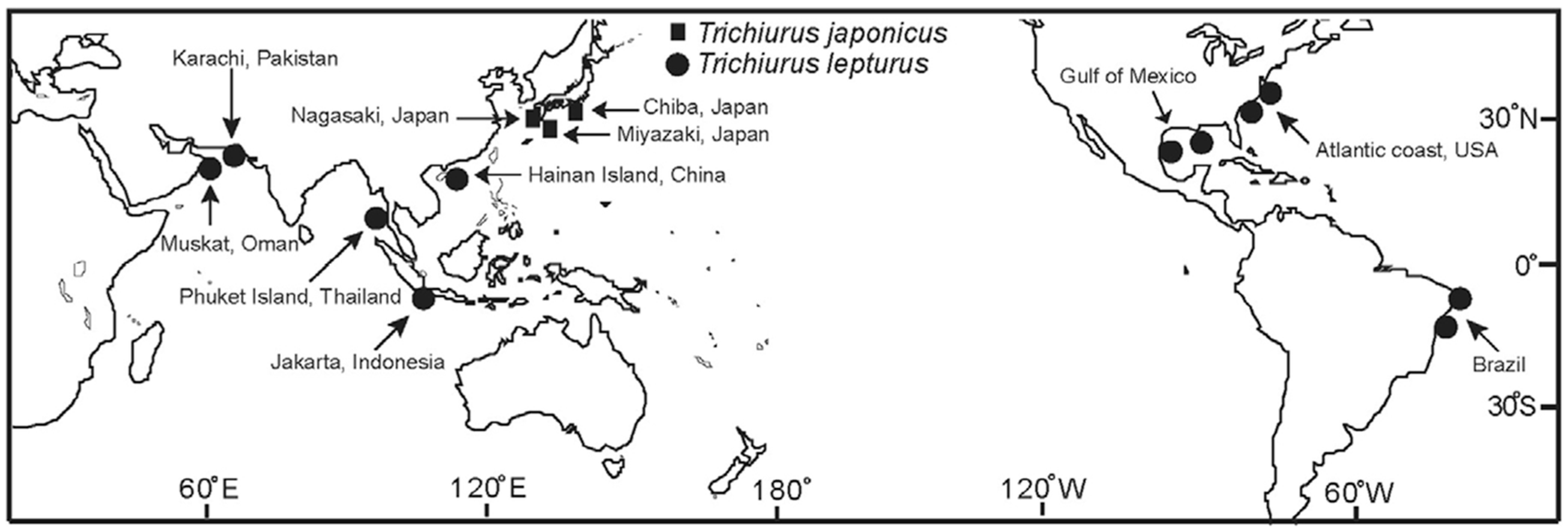
Figure 2.
Estimated average predictive difference of marginal growth index (MGI) for cutlassfish (T. spp.) in variability spatial scale (i.e. distance to land (km): coastal < 20 nm, inner shelf 20–80 nm, outer shelf 80–120 nm, and shelf break 120–350 nm) in the seas of Japan/East Sea from April to December.
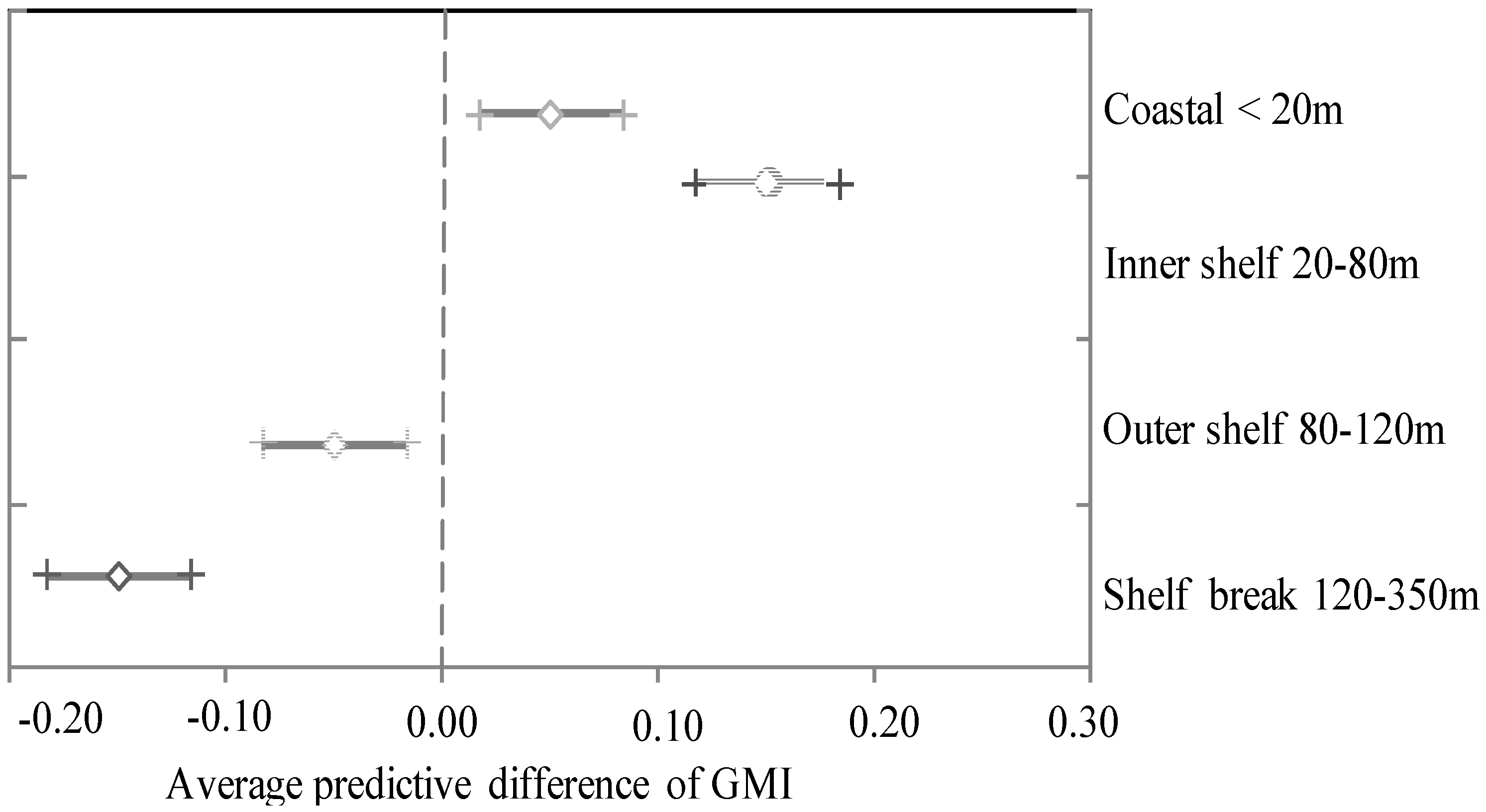
Figure 3.
The Catch-MSY model parameters, such as intrinsic growth rate (r), maximum sustainable yield (MSY) and carrying capacity (k), with their relations to catch variability were analyzed for T. japonicas in the ECS. (a) The time series of catches with overlaid estimates of MSY (the limits contain about 95% of the estimates). (b) Prior uniform distribution of r–k (the black dots denote the posterior combinations). (c) The relationship between ln(r) and ln(k) with the geometric mean MSY (95% of the estimates). (d–f) Posterior densities of r, k, and MSY (the limits contain about 95% of the estimates).
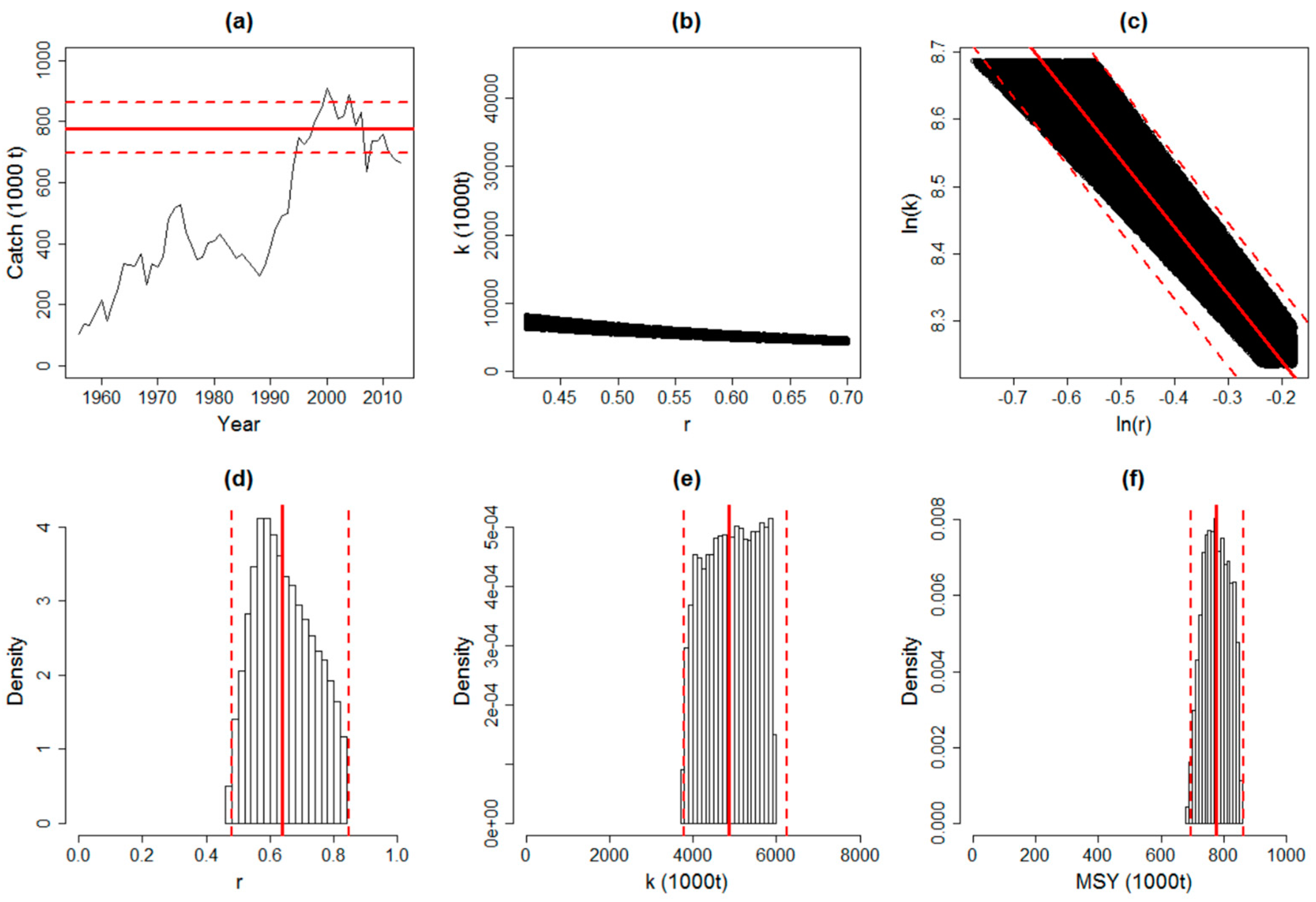
Figure 4.
Spawning and feeding migration index (SFMI) for different size classes (i.e. preanal lengths (mm): 80–200, 201–280, 281–400, and > 400) of T. japonicas divided according to season (i.e., in summer and winter). Note that the vertical bars denote the standard deviation.
Figure 4.
Spawning and feeding migration index (SFMI) for different size classes (i.e. preanal lengths (mm): 80–200, 201–280, 281–400, and > 400) of T. japonicas divided according to season (i.e., in summer and winter). Note that the vertical bars denote the standard deviation.
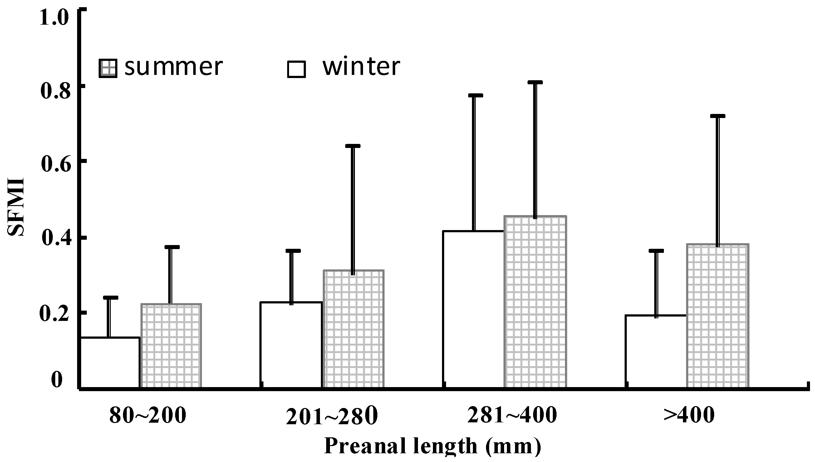
Figure 5.
Mean sea level trends determined from altimetry alone from 1993 to 2010. Note that the highest latitudes are not included.
Figure 5.
Mean sea level trends determined from altimetry alone from 1993 to 2010. Note that the highest latitudes are not included.
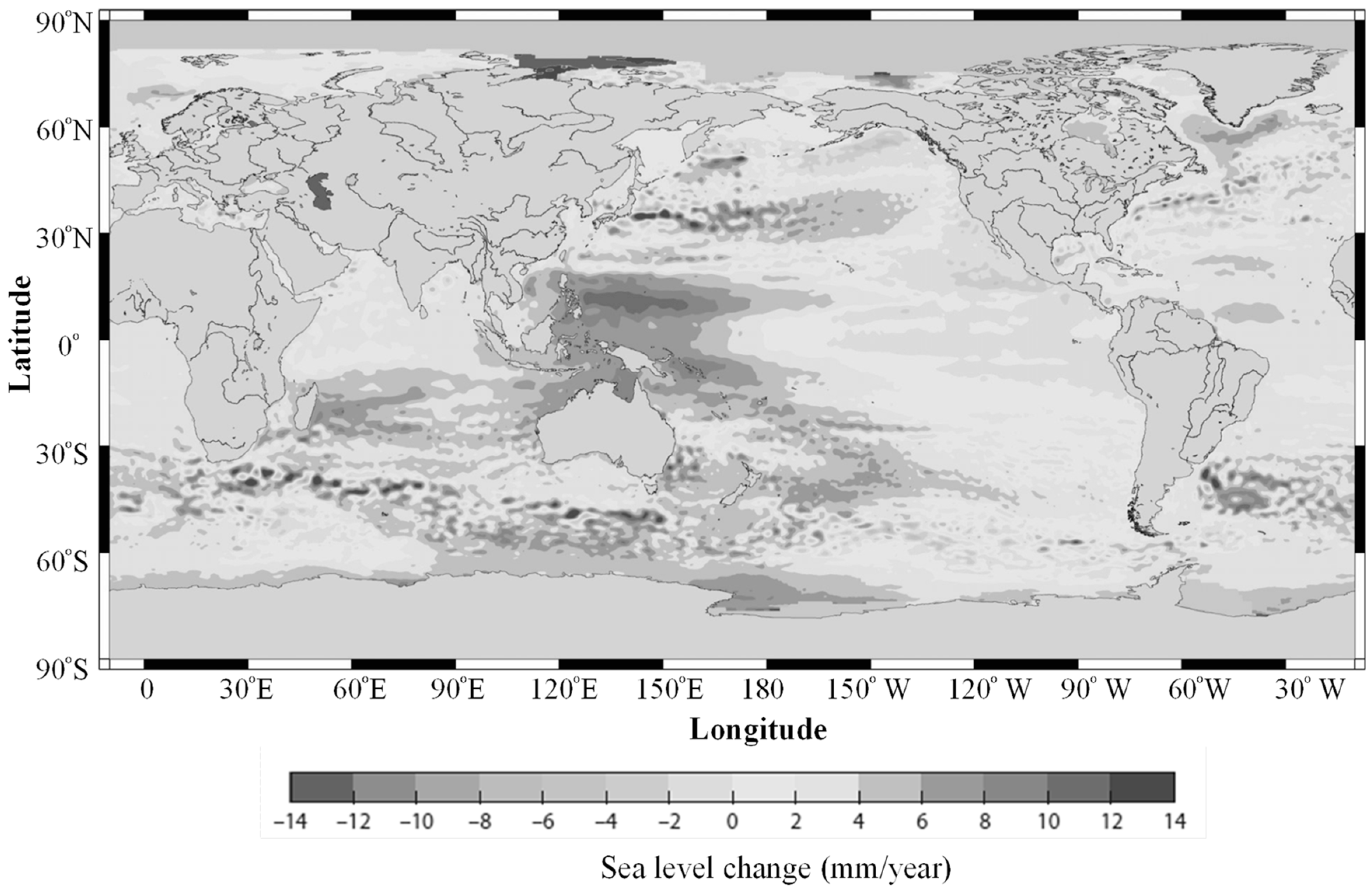
Figure 6.
Effective population sizes of cutlassfish (T. spp.) of the different geographic groups (e.g. ECS, YS, and BH) using the mitochondrial cytochrome b sequences.
Figure 6.
Effective population sizes of cutlassfish (T. spp.) of the different geographic groups (e.g. ECS, YS, and BH) using the mitochondrial cytochrome b sequences.
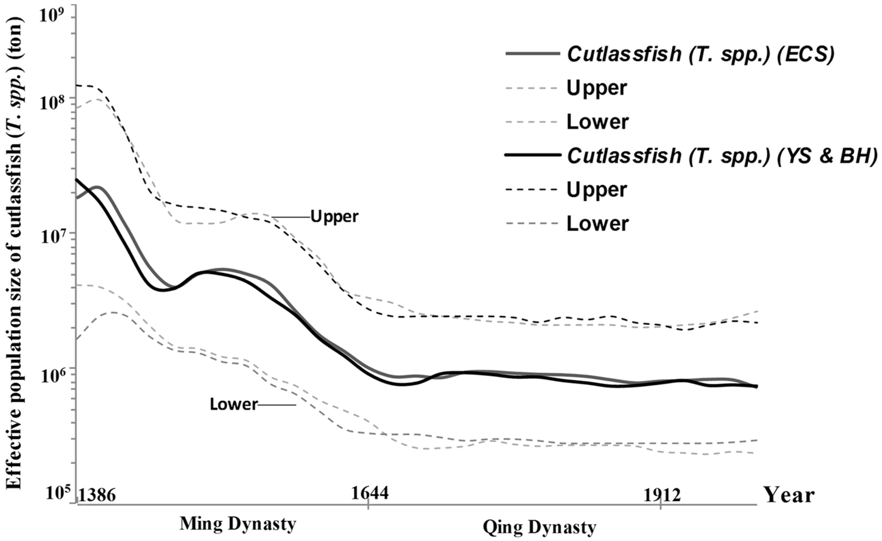
Figure 7.
Mean and 80% confidence intervals for the distributions of water temperature, salinity, depth, and distance to land (km) perfected to the cutlassfish (T. spp.) in the northwest Pacific Ocean, including ECS, SCS, YS, BH, and seas of Japan/East Sea separated according to summer and winter seasons.
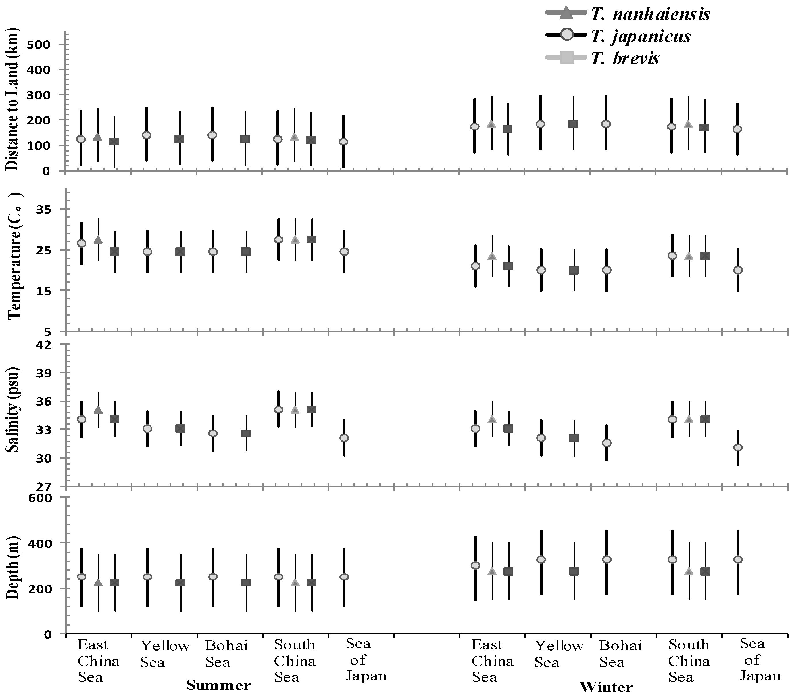
Figure 8.
(a) Biomass (g m-2) of epipelagic (0-100 m) mid-trophic functional groups (i.e., prey) in the Pacific Ocean (including Seas in China and Seas of Japan/East Sea) (daytime). (b) Biomass (g m-2) of mesopelagic (100-400 m) mid-trophic functional groups (i.e., prey) in the Pacific Ocean (including Seas in China and Seas of Japan/East Sea) (daytime) (1992–2004).
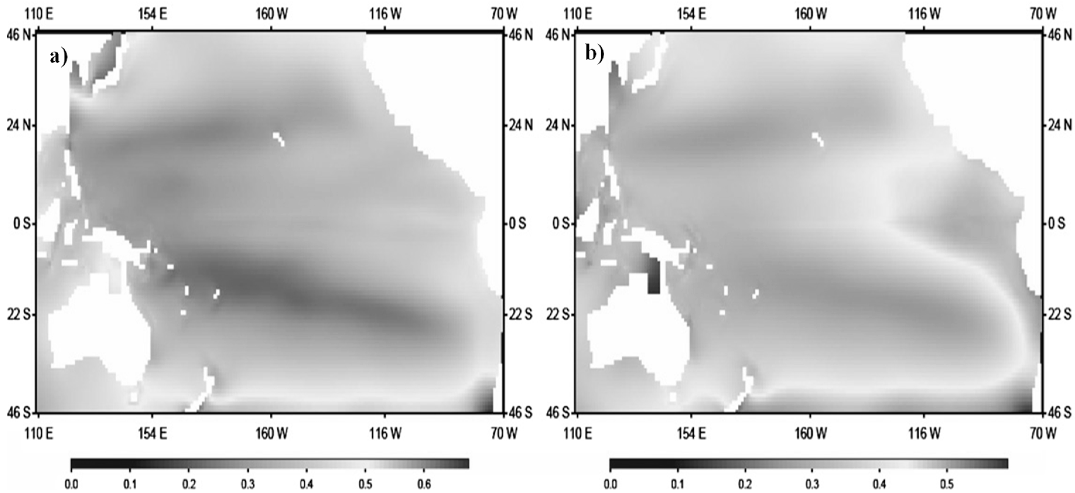

Table 1.
Summary of the three species groups of cutlassfish (Trichiurus spp.) in the northwest Pacific Ocean, including seas in China [i.e., South China Sea (SCS), East China Sea (ECS), Yellow Sea (YS) and Bohai Sea (BH)], and southern Seas of Japan/East Sea.
Table 1.
Summary of the three species groups of cutlassfish (Trichiurus spp.) in the northwest Pacific Ocean, including seas in China [i.e., South China Sea (SCS), East China Sea (ECS), Yellow Sea (YS) and Bohai Sea (BH)], and southern Seas of Japan/East Sea.
| Valid Name | Scientific name (by Authors) |
Distribution | Reference |
|---|---|---|---|
| Trichiurus japonicas | T. lepturus (Linnaeus,1758) | Circumtropical and temperate waters (e.g. ECS, BH, YS, and the Seas of Japan/East Sea ) | El-Haweet, 1996 Shih, 2004 Zeng 2005 Liu et al 2009 Jin et al. 2010 |
| T. lepturus japonicas (Temmick&Schlegel,1844) | |||
| T. japonicas (Temmick&Schlegel,1844) | |||
| T. japanicus (Temmick&Schlegel,1844) | |||
|
Trichiurus brevis |
T. minor (Wang et al. 1993) | Northwest Pacific (e.g. ECS, SCS) | Wang et al. 1993 Zeng 2005 |
| T. brevis (Wang & You, 1992) | |||
|
Trichiurus nanhaiensis |
T. lepturus (Chakraborty et al. 2006) T. nanhaiensis (Wang & Xu, 1992) |
West Pacific (northwest SCS) | Wang& Xu, 1992 Kwok & Ni, 2000 |
Table 2.
Summary statistics for results of length–weight relationship parameters and growth parameters of the cutlassfish (Trichiurus spp., Linnaeus, 1758).
Table 2.
Summary statistics for results of length–weight relationship parameters and growth parameters of the cutlassfish (Trichiurus spp., Linnaeus, 1758).
| Trichiurus | Trichiurus | Trichiurus | Reference | |
|---|---|---|---|---|
| japonicas | nanhaiensis | brevis | ||
| East China Sea | κ=(0.27, 0.46) yr−1 | κ=(0.17, 0.22) yr−1 | κ=(0.11, 0.17) yr−1 | Shih et al. 2011 |
| W∞=(1911.3, 1950.2)g | W∞=(2998.8, 3144.4)g | W∞=(2685.4, 2871.4)g | Lin et al. 2006b | |
| Lam=(43.2, 46.3) cm | Lam=(45.7, 54.9) cm | Lam=(38.7, 41.6) cm | Tzeng et al. 2007 | |
| PL∞=(54.1, 85.1)cm | PL∞=(60.1, 89.1)cm | PL∞=(42.3, 49.8)cm | - | |
| t0 =(-1.762, -0.634) | t0 =(-1.762, -0.634) | t0 =(-1.762, -0.634) | Shih et al. 2011 | |
| a=(0.00032, 0.00054) | a=(0.00032, 0.00054) | a=(0.00079, 0.00481) | - | |
| b=(3.06, 3.22) | b=(3.06, 3.22) | b=(2.92, 3.32) | - | |
| South China Sea | κ=(0.17, 0.22) yr−1 | κ=(0.11, 0.17) yr−1 | Shih et al. 2011 | |
| W∞=(2998.8, 3144.4)g | W∞=(2685.4, 2871.4)g | Kwok & Ni, 2000 | ||
| Lam=(45.7, 54.9) cm | Lam=(38.7, 41.6) cm | - | ||
| PL∞=(60.1, 89.1)cm | PL∞=(42.3, 49.8)cm | Shih et al. 2011 | ||
| t0 =(-1.762, -0.634) | t0 =(-1.762, -0.634) | - | ||
| a=(0.00032, 0.00054) | a=(0.00079, 0.00481) | Wang et al. 2011a | ||
| b=(3.06, 3.22) | b=(2.92, 3.32) | - | ||
| Yellow Sea & Bohai Sea | κ=(0.27, 0.46) yr−1 | Shih et al. 2011 | ||
| W∞=(1961.3, 1989.2)g | Lin et al. 2006b | |||
| Lam=(43.5, 46.8) cm | Tzeng et al. 2007 | |||
| PL∞=(55.2, 86.9)cm | - | |||
| t0 =(-1.762, -0.634) | Shih et al. 2011 | |||
| a=(0.00032, 0.00054) | - | |||
| b=(3.06, 3.22) | - | |||
| Sea of Japan | κ=(0.17, 0.22) yr−1 | Shih et al. 2011 | ||
| W∞=(1891.6, 1918.5)g | Lin et al. 2006b | |||
| Lam=(41.3, 42.6) cm | El-Haweet & Ozawa, 1996 | |||
| PL∞=(50.2, 86.3)cm | - | |||
| t0 =(-1.975, -1.791) | Shih et al. 2011 | |||
| a=(0.00032, 0.00054) | - | |||
| b=(3.06, 3.22) | - |
Note: PL is the preanal length, Lam is the length at first maturity, W is the whole-body wet weight (W), t0 is the theoretical age at Lt = 0, κ is the growth coefficient, and a and b are the parameters of the length–weight relationship.
Table 3.
Summary of main categories of prey groups and regional feeding distributions of the cutlassfish (Trichiurus spp., Linnaeus, 1758).
Table 3.
Summary of main categories of prey groups and regional feeding distributions of the cutlassfish (Trichiurus spp., Linnaeus, 1758).
| Summary | Regional scales |
Feeding area |
Prey composition |
|---|---|---|---|
|
BH & YS (T. japonicas) |
35°N-45°N and 117°E-123°E |
Few high abundance area (Nowadays only as bycatch) |
Fishes(e.g. engraulis japonicus, apogon lineatus, T. japonicus), cephalopod (e.g. loligo japonica, sepiellamaindroni de), macrura |
|
ECS (T. japonicas) |
23°N-34°N and 117°E-131°E |
30°N-31°N and 123°E-124°E |
Pisces (e.g. T. japonicas, decapterus maruadsi), crustacea (e.g. mysidacea, stomatopoda, euphausiacea) cephalopods (e.g. abralia multihamata), urochorda. |
|
SCS (T. brevis and T. nanhaiensis) |
11°N-22°N and 109°E-117°E |
22°N-24°N and 109°E-110°E |
Fishes (e.g. Benthosema pterotum, Bregmaceros lanceolatus, Encrasicholina heteroloba, sardinella longiceps, decapterus russelli), crustaceans (e.g. acetes sp., unidentified shrimps), cephalopod (loligo sp.) |
|
Through the Korea Strait into the East Japan Sea (T. japonicas) |
31°N-40°N and 127°E-150°E |
35°N-38°N and 128°E-145°E |
Fishes(e.g. T. japonicas, engraulis japonicus, apogon lineatus), crustaceans (e.g. Euphausiids, shrimps) cephalopod (e.g. loligo japonica, sepiellamaindroni de), chaetognaths |
Table 4.
Correlation analysis between environmental factors and catch per unit effort (CPUE) of cutlassfish (Trichiurus spp.) in China seas and the distributions of the factors (i.e. depth, temperature, salinity, primary production, and distance to land).
Table 4.
Correlation analysis between environmental factors and catch per unit effort (CPUE) of cutlassfish (Trichiurus spp.) in China seas and the distributions of the factors (i.e. depth, temperature, salinity, primary production, and distance to land).
| Correlation Analysis | Partial correlation coefficient | Correlation coefficient (R) | P-Significance (2-tailed) | |
|---|---|---|---|---|
| Sea surface temperature (ECS) & CPUE (ECS) | 0.52 (3); 0.50 (5) | -0.67 | 0.01 | |
| Summer wind speed (ECS) & CPUE (ECS) | 0.46 (0); 0.38 (2) | -0.42 | 0.02 | |
| Winter wind speed (ECS) & CPUE (ECS) | - 0.42 (1); - 0.33 (2) | 0.41 | 0.04 | |
| Winter wind speed (YS) & CPUE (ECS) | - 0.44 (3); - 0.50 (4) | 0.47 | <0.001 | |
| Summer wind speed (YS) & CPUE (ECS) | - 0.66 (2); - 0.49 (3) | -0.45 | <0.001 | |
| Annual precipitation (ECS) & CPUE (ECS) | 0.48 (1); 0.56 (2) | -0.37 | <0.001 | |
| Factors distributions | Min | Pref Min (10th) | Pref Max (90th) | Max |
| Depth (m) | 0 | 100 | 350 | 400 |
| Temperature (C°) | 8.31 | 18.45 | 28.39 | 29.39 |
| Salinity (psu) | 22.7 | 32.27 | 35.93 | 39.36 |
| Primary Production | 0 | 488 | 1957 | 4336 |
| Distance to Land (km) | 0 | 10 | 209 | 1463 |
Disclaimer/Publisher’s Note: The statements, opinions and data contained in all publications are solely those of the individual author(s) and contributor(s) and not of MDPI and/or the editor(s). MDPI and/or the editor(s) disclaim responsibility for any injury to people or property resulting from any ideas, methods, instructions or products referred to in the content. |
© 2024 by the authors. Licensee MDPI, Basel, Switzerland. This article is an open access article distributed under the terms and conditions of the Creative Commons Attribution (CC BY) license (http://creativecommons.org/licenses/by/4.0/).
Copyright: This open access article is published under a Creative Commons CC BY 4.0 license, which permit the free download, distribution, and reuse, provided that the author and preprint are cited in any reuse.


