Use of Vegetation Activity Index for Evaluation of L-Alpha Amino Acid Treatment in Sugarcane

1. Introduction

Sugarcane plays an important role in food and energy production in Brazil and the world (dos Santos Luciano et al., 2021). Currently, Brazil is the largest producer of sugarcane in the world, with self-sufficiency in the use of ethanol as a biofuel, in addition to being one of the largest suppliers of sugar to the world (Vasconcelos et al., 2023). Sugarcane is a perennial crop that contributes to almost 80% of global sugar products. Therefore, sugarcane producers and food companies are searching for ways to address concerns related to the yield and health of the sugarcane crop (Akbarian, 2020). Given that sugarcane crops often occupy large areas in countries such as Brazil, the development of tools capable of being operated remotely benefits the management of this crop in the field, avoiding laborious and time-consuming sampling and promoting the reduction of operation costs (Vasconcelos et al., 2023).

The vastness of sugarcane plantations makes real-time performance evaluation challenging when using traditional monitoring tools. Thus, modern approaches based on aerial images obtained by satellite or by remotely piloted aircraft systems (RPAS) may be viable options for surveying vast portions of sugarcane-cultivated land cheaply and quickly (Vasconcelos et al., 2023). In Brazil, the prediction of the total amount of sugarcane production involves a survey of agricultural production that is carried out using information from regional peculiarities, agronomic aspects, and monthly data from national institutes, producers, and other collaborators in the sector (dos Santos Luciano et al., 2021). However, these techniques have limits in terms of spatial variability and forecasting capabilities. New methods for estimating sugarcane yield were tested, based on locally available information on soils, climate, and vegetation conditions.

Measuring a biophysical parameter of the plant in the field is extremely difficult and requires a lot of time and labor. In the case of a larger geographical area, it may be impossible when relying on field measurements. To solve this problem, ongoing efforts have been made to develop methodologies for estimating biophysical parameters of crops using satellite data. Satellite data act as a single and convenient source for detailed knowledge of spatial and temporal variation of crop biophysical parameters. There are three approaches in three categories for sugarcane yield models: mechanistic-type crop growth simulators, statistical-based crop climate analysis models, and RS-based models. The spectral reflectance of crop fields always varies in relation to the phenology, type of stage, and health of the crop, and these can be well observed and measured using multispectral sensors.

Worldwide, satellite imagery is widely used to predict sugarcane yield (Verma et al., 2020). Predictive models of sugarcane growth and yield are essential for government planning and provide valuable information for producers, improving crop production, reducing costs, and assisting in crop management and logistics (dos Santos Luciano et al., 2021). Accurate forecasting of agricultural yield is critical for sustainable agricultural planning and for ensuring food security in regions critically affected by climate change and extreme weather events. Existing regression-based crop yield estimation approaches typically rely on a specific set of predictor variables (Dimov et al., 2022). Early forecasting of sugarcane crop yield would benefit sugarcane producers and policymakers by enabling timely decisions (Akbarian, 2022). Estimating acreage and forecasting yield before harvest are of paramount importance for nations with well-organized agricultural and food economies.

The applications of remote sensing in assessing discrimination vigor and estimating yield are significant (Verma et al., 2020). Traditional data collection methods for crop vigor assessment and yield estimation, based on field surveys or crop cutting trials, are subjective; lack spatial coverage; are often expensive, time-consuming, and prone to large errors due to incomplete soil observation, leading to poor crop yield assessments (Verma et al., 2020). Remote sensing techniques provide an effective system for monitoring vegetation dynamics at multiple scales using vegetation indices (VI), calculated from remote sensing reflectance measurements in the visible and infrared regions of the electromagnetic spectrum (Carreño-Conde et al., 2021).

The Normalized Difference Vegetation Index (NDVI) is often used for vegetation mapping, crop status indication, biomass estimation, drought monitoring, and evapotranspiration (Carreño-Conde et al., 2021). NDVI quantifies vegetation health by measuring the difference between near-infrared (strongly reflected) and red (absorbed) light (Carreño-Conde et al., 2021). This relationship between NDVI and vegetation health is well known and used in studies for vegetation mapping, as an indicator of crop status, as a biomass estimator, and for drought or evapotranspiration monitoring (Carreño-Conde et al., 2021). High spatial resolution and high temporal frequency of vegetation indices are essential to describe and analyze spatial patterns in vegetation monitoring and management (Liao et al., 2017).

Variations in aerial images of cultivated canopies are tracked using vegetation indices calculated from wavelength band data collected during different stages of crop development, in different locations and in cultivated fields adopting different agricultural practices. Therefore, small variations in growth conditions can be identified, compared, and correlated by applying mathematical models. These vegetation indices are typically obtained using mathematical combinations between spectral band data from proximal, suborbital, and orbital sensors that are related to the amount and stage of vegetation development in the area where the spectral measurement was collected (Vasconcelos et al., 2023).

Vegetation indices have been increasingly used to characterize biophysical parameters, such as leaf area and green biomass, which indicate the presence and condition of vegetation at a given time due to their strong correlation with absorbed sunlight (Vasconcelos et al., 2023). These indices can differentiate vegetated areas from non-vegetated areas, as well as identify stages of the phenological cycle of specific agricultural crops (Shukla, 2021).

Rojo Baio et al. (2029) used NDVI to determine the effect of soil chemical attributes, soil type, and precipitation on cotton yields and yield variability. The wide availability of satellite sensors and advanced data processing techniques has improved sugarcane yield forecasting at local and global scales, but more work is needed to explore the synergy between remote sensing, meteorological, and agronomic data (dos Santos Luciano et al., 2021). In-season yield forecasting and monitoring using vegetation indices fills the gap of the lack of high-precision sensor data over large areas, such as soil moisture, temperature, and rainfall, instead of using the farm-level yield forecasting accurate model (Supavetch, 2022).

Remote sensing (RS) technology plays a crucial role in providing advanced, seasonal information on acreage, vigor, and production before actual harvesting in an object-oriented manner. It provides information about the actual status of cultures and makes use of their inherent spatial quality to describe biophysical processes in space and time (Verma et al., 2020). NDVI measures total green biomass at any given time, serving as an indicator of sugarcane crop growth, and is related to plant biomass and yield (Verma et al., 2020). The system fertilization approach aims to improve the efficiency of nutrient use on agricultural land by taking advantage of the nutrient cycle within an agroecosystem. NDVI is a promising methodology for assessing plant biomass and nutrient content (Farias et al., 2023).

Changes in morphophysiological characteristics due to biotic or abiotic stresses in sugarcane are laborious and time-consuming to measure in soil. Predicting these characteristics using aerial imagery is important for detecting stress and timely management (Poudyal et al., 2023). Multispectral data in the visible and near-infrared light range are used to calculate vegetation indices as predictors of cereal grain yield (Panek & Dariusz Gozdowski, 2021). Panek and Dariusz Gozdowski (2021) found that the cumulative mean NDVI provides more stable grain yield predictions per season. Som-Ard et al. (2021) reviewed applications of remote sensing technology in the sugarcane sector, highlighting the high potential of Earth observation (EO) data for sugarcane mapping, crop growth anomaly detection, health monitoring, and yield estimation. They pointed out that: (1) optimal results require dense time series of multiple satellites and between measurement modalities; (2) the lack of human resources in many sugarcane-producing countries often leads to difficulties in cultivation, suggesting that state-of-the-art remote sensing technology could benefit the sugarcane industry and the broader agricultural sector by making it more attractive to people.

Global warming has resulted in increased meteorological droughts, affecting vegetation growth with social and economic consequences (Ding et al., 2022). The use of seaweed-based bioproducts has been gaining momentum in crop production systems due to their unique bioactive components and effects. They have phytostimulatory properties that result in increased plant growth and yield parameters in several important crop plants (Ali et al., 2021). Amino acid metabolism plays a crucial role in sugarcane drought response mechanisms, affecting signaling, osmoregulation, and maintenance of energy balance, providing carbon skeletons to the tricarboxylic acid cycle, helping plant survival during stress and recovery after stress (Diniz et al., 2020; Ali et al., 2021).

Biostimulants are substances or microorganisms applied to plants with the aim of increasing growth, productivity, and resistance to biotic stresses (caused by living organisms, such as pests and diseases) and abiotic stresses (caused by environmental factors, such as drought, salinity, and extreme temperatures) (Du Jardin, 2015). They may include compounds such as amino acids, seaweed extracts, humic and fulvic acids, as well as beneficial microorganisms such as bacteria and fungi (Calvo et al., 2014).

Sugarcane is susceptible to a variety of pests and diseases that can significantly impact its productivity. Biostimulants can help mitigate these effects by several mechanisms, such as: boosting the plant’s immune system; improving soil health by activating beneficial microorganisms that can improve soil structure and increase nutrient availability, thereby promoting a healthy environment for plant growth; inducing systemic resistance, protecting the plant against a wide range of pathogens (Vessey et al., 2003; Pieterse et al., 2014). Abiotic stresses such as drought, salinity, and temperature fluctuations can also negatively impact sugarcane productivity.

Biostimulants can play a crucial role in mitigating these stresses by increasing the plants’ ability to retain water and improving water use efficiency by helping plants withstand periods of drought (Rouphael et al., 2015). They can also help the plant maintain ionic balance and reduce the toxic effects of soil salinity by promoting healthy growth in saline conditions (Ashraf & Foolad, 2007). These substances can also increase the resistance of plants to extreme temperatures by protecting plant cells from heat-induced damage (Hasanuzzaman et al., 2013). Reports published so far have confirmed the positive effects on plant growth, vigor, improved tolerance to pests, diseases, and abiotic stresses, as well as an overall improvement in plant productivity (Ali et al., 2021).

The effects of foliar application of biostimulants on sugarcane exposed to water stress, particularly on plant metabolism, stalk and sugar yields, broth purity, and sugarcane technological quality, have received little attention (Chen et al., 2021; Jacomassi et al., 2022; Rao et al., 2022). Chen et al. (2021) reported that spraying seaweed extract (SEW) at different stages of sugarcane growth led to yield increases ranging from 3.33% to 9.23% and contributed to a 5.00% increase in sucrose content. Raju et al. (2022) observed productivity increases from 15.2% to 18.5% in sugarcane when applying SEW in drought conditions. Similarly, Jacomassi et al. (2022) found that foliar application of SEW can relieve drought stress while improving sugarcane development, stalk productivity, sugar production, and plant physiological and enzymatic processes. Their studies concluded that SEW mitigated the negative effects of drought stress and increased stalk productivity per hectare by up to 3.08 Mg ha-1. Moreover, SEW increased the accumulation of sucrose in the stalk, resulting in an increase in sugar productivity of 3.4 kg Mg-1 per hectare and higher industrial quality of the raw material. Productivity maps are essential for precision agriculture (PA) practices, but on-board productivity monitoring for sugarcane is challenging (Canata et al., 2021).

Assessing spatial variability in sugarcane crops is difficult due to limited adapted solutions for productivity mapping (Canata et al., 2021). Yield maps help to understand variability within the field, delimit management zones, and improve site-specific management strategies (Bramley et al., 2019; Jeffries et al., 2019; Momin et al., 2019). Vasconcelos et al. (2023) demonstrated that spectral indices such as NDVI and Visible Atmospherically Resistant Index (VARI) are related to sugarcane yield, showing that high values of these indices are associated with higher yield. Shammi and Meng (2021) developed crop growth metrics using time series NDVI for soybean yield modeling, achieving 95% accuracy in yield predictions using a cross-validation approach.

The model developed by Supavetch (2022) for industrial scale, using only NDVI, is used by sugarcane plants for business planning and operational control processes, such as in the correct planning of sugarcane supply to the power plants and in the optimization of sugarcane supply logistics. The main objective of this study is to use the Vegetation Activity Index (VAI) obtained from NDVI evaluations in various crop periods to evaluate the effect of amino acid treatment on sugarcane. Specifically, the objectives of this study are:

To calculate and integrate NDVI: collecting NDVI data at different stages of sugarcane growth and integrating these values over time to obtain a cumulative measure of vegetation activity.

To evaluate the efficacy of amino acid treatment: comparing VAI values between areas treated with L-alpha amino acids and control (untreated) areas to determine whether there is a significant positive impact on green biomass and plant health.

To validate results with field measurements: performing additional field measurements to validate NDVI data and ensuring accuracy of analyses by correlating them with traditional agronomic parameters.

To analyze vegetation dynamics: observing and analyzing temporal variations in VAI to better understand how amino acid treatment affects the dynamics of sugarcane growth and development throughout the crop cycle.

To develop a robust methodology: proposing a robust methodology to use NDVI and its temporal integration as an efficient and non-invasive tool to assess vegetative state and manage agricultural crops.

2. Material and Methods

2.1. Evaluation of Product Use

The studied product is a biostimulant developed to improve vegetative growth and recovery of plants subjected to abiotic and biotic stresses. Its formulation includes a combination of macro and micronutrients complexed with L-alpha amino acids and seaweed extracts. This composition aims to accelerate plant metabolism, promoting rapid and balanced nutrition at the cellular level, which is essential for a healthy plant growth. presents the composition of the biostimulant.

Table 1. L-alpha amino acid composition.

Nutrient	%	g/L	Source
Water soluble nitrogen	1.00	11.0	Urea
Water soluble phosphorus	10.40		Food phosphoric acid
Water soluble potassium	2.00		Potassium sulphate
Total organic carbon	6.00		Glucose syrup
Amino acids	0.63		Plant sources

Table 1. L-alpha amino acid composition.

Nutrient	%	g/L	Source
Water soluble nitrogen	1.00	11.0	Urea
Water soluble phosphorus	10.40		Food phosphoric acid
Water soluble potassium	2.00		Potassium sulphate
Total organic carbon	6.00		Glucose syrup
Amino acids	0.63		Plant sources

The dosage used was 2.0 l.ha^-1 and the mode of application was by aerial spraying; its marketing price is 65.00 R$.l^-1.

For the product evaluation, 9 portions were selected according to and detailed in . All portions are on the 4th cut, were harvested in June 2023, and are grown with the RB855453 variety.

Figure 1. Digital relief model of the area where the experiment was conducted.

Figure 1. Digital relief model of the area where the experiment was conducted.

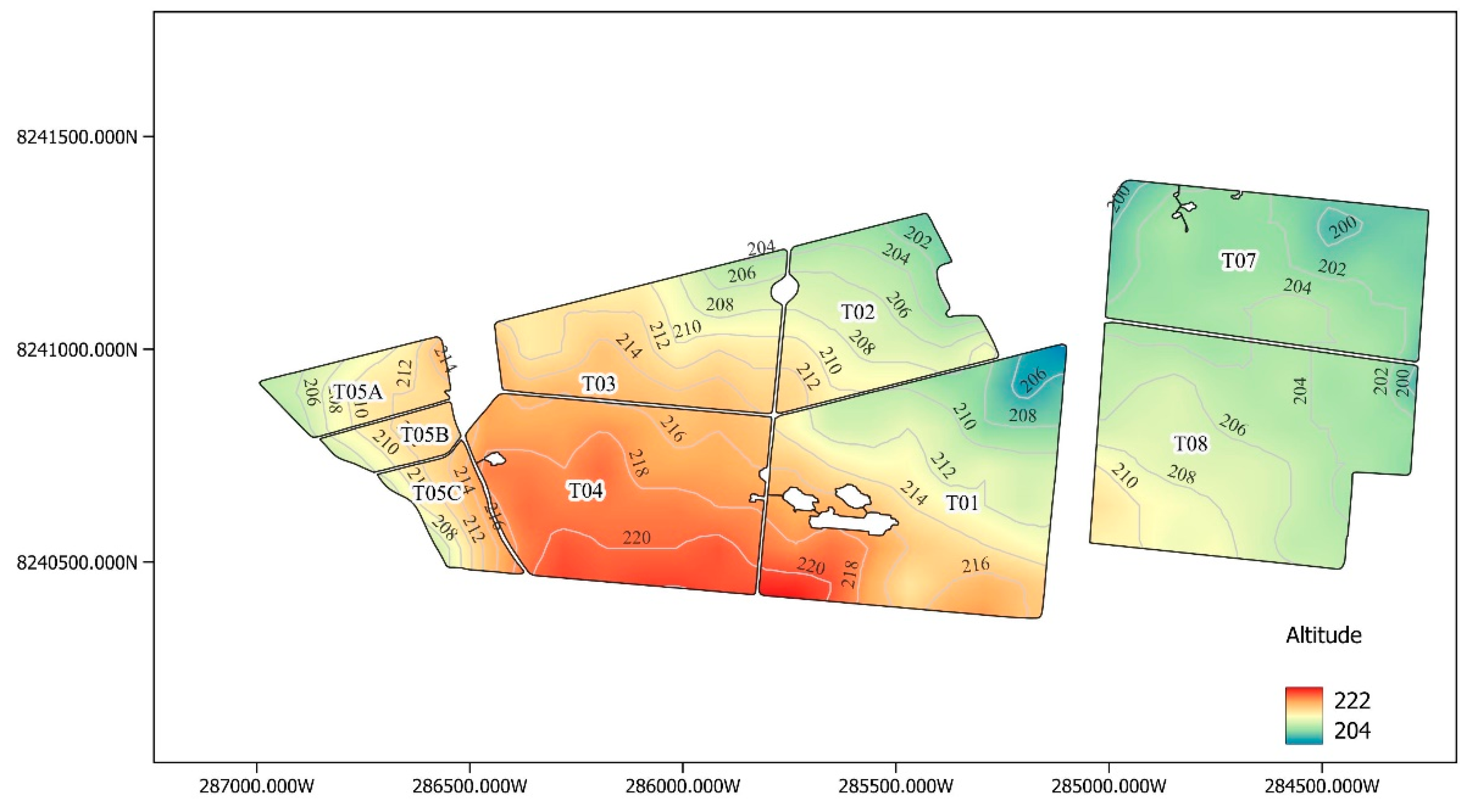
Table 2. Identification of the plots that make up the experiment.

Plot	Area
Treated
01	34.06
02	15.20
03	17.72
04	26.41
Total plots treated	93.39
Control
05th	6.00
05B	3.05
05C	4.74
07	28.87
08	33.96
Total plots control	76.62

Table 2. Identification of the plots that make up the experiment.

Plot	Area
Treated
01	34.06
02	15.20
03	17.72
04	26.41
Total plots treated	93.39
Control
05th	6.00
05B	3.05
05C	4.74
07	28.87
08	33.96
Total plots control	76.62

2.2. NDVI values Collected for Multiple Dates

For the analysis of vegetation temporal variation, the collection of NDVI values was carried out in several dates. The images used to calculate the NDVI were obtained from the Planet satellite constellation, which provides high-resolution images with high temporal frequency, which is crucial for monitoring rapid changes in vegetation.

2.3. Collection and Processing Procedures

The satellite images were processed using QGIS software, an open source tool widely used in geographic information systems (GIS). QGIS allows the processing and analysis of images efficiently, being suitable for the execution of NDVI calculations due to its raster processing capabilities.

2.4. Process Steps

Image acquisition: Satellite images were acquired directly from the Planet constellation at predefined time intervals to cover the study period.

Image preprocessing: The preprocessing included atmospheric correction, geometric correction, and clipping of the areas of interest. These steps ensure the accuracy and quality of the data for subsequent analysis.

NDVI calculation: Using QGIS, NDVI was calculated for each image. NDVI is determined by .

$$\mathit{N}\mathit{D}\mathit{V}\mathit{I}={\displaystyle \frac{\mathit{N}\mathit{I}\mathit{R}-}{\mathit{N}\mathit{I}\mathit{R}+}}$$

(1)

• In which:
• NDVI: normalized difference vegetation index;
• NIR: near-infrared reflectance;
• Red: reflectance in red.

Data storage and organization: The calculated NDVI values were organized in a structured database, associating each value with its respective acquisition date. This allows an efficient temporal analysis and facilitates the visualization of vegetation variation trends over the studied period.

Considerations: The collection and processing of NDVI data from the Planet constellation images and the use of QGIS for the calculation of the index provided a robust database for subsequent analysis. The accuracy and frequency of the data obtained are fundamental to monitor vegetation dynamics and better understand the spatial and temporal patterns involved.

2.5. Data Preparation

NDVI data were prepared in a tabular format, in which each row represents a specific date and the corresponding column presents the NDVI value for that date - .

Table 3. Organization of NDVI data.

Date	NDVI
t1	NDVI1
t2	NDVI2
t3	NDVIn

Table 3. Organization of NDVI data.

Date	NDVI
t1	NDVI1
t2	NDVI2
t3	NDVIn

2.6. Second Degree Polynomial Regression

To model the variation of NDVI over time, it was decided to adjust a second degree equation to the collected data. The second degree polynomial regression was chosen for its ability to capture the nonlinear trend of NDVI data over the different observed dates. The function to be adjusted is of the type shown in .

$${\mathit{N}\mathit{D}\mathit{V}\mathit{I}}_{\mathit{t}}=\mathit{a}\ast {\mathit{t}}^2+\mathit{b}\ast \mathit{t}+\mathit{c}$$

(2)

• In which:
• NDVI_t: NDVI value adjusted over time;
• t: dates;
• a, b, c: coefficients to be determined from the data.

2.7. Polynomial Regression Adjustment

Using second-degree polynomial regression techniques, curve adjustment to the data was performed to find the values of the coefficients a, b, and c that best describe the variation of NDVI over time. The Real Statistics software, an additional tool for Excel, was used to perform the polynomial regression.

2.8. Steps for Curve Adjustment

Data preparation: The NDVI values and their respective dates were organized in an Excel spreadsheet. The dates column was transformed into a numeric variable representing the time (t).

Calculation of coefficients: Real Statistics performed curve adjustment by calculating the coefficients a, b, and c, which minimize the sum of the squares of the residuals between the observed values and the adjusted values of NDVI.

Model evaluation: After obtaining the coefficients, the quality of the adjustment was evaluated using statistical metrics such as the coefficient of determination (R²), which indicates the proportion of variability of the NDVI data explained by the adjusted model.

2.9. Integration of the Function to Obtain the Area under the Curve

The integration of the function to obtain the area under the curve of NDVI is the main approach of this study. This methodology not only improves accuracy in assessing plant health and vigor, but also presents a new approach to the analysis of large-scale agricultural experiments.

Historically, vegetation assessment has relied on punctual measurements of NDVI, which provide a limited and instantaneous view of plant activity (Jiang et al., 2020; Jin et al., 2021; Liang et al., 2023). In contrast, the methodology proposed in this study involves the integration of NDVI values over time, resulting in a more robust and representative Vegetation Activity Index (VAI). The integration allows the summation of NDVI values at defined time intervals, providing a comprehensive and continuous view of vegetation dynamics.

The originality of this approach lies in the ability to accurately capture and quantify temporal variations in plant biomass and photosynthetic activity. By calculating the area under the NDVI curve, we obtain an integrated measure that more faithfully reflects the vegetative state of crops throughout the entire growth cycle rather than relying on punctual measurements.

To calculate the area under the NDVI curve over time, was integrated, and the integral of NDVI_t between two points t₁ and t_n is given by (3.

$${\int }_{{\mathit{t}}_1}^{{\mathit{t}}_{\mathit{n}}}\left(\mathit{a}\ast {\mathit{x}}^2+\mathit{b}\ast \mathit{x}+\mathit{c}\right)\mathit{d}\mathit{t}$$

(3)

The calculation of the integral results in (4:

$${\displaystyle \frac{\mathit{a}}{3}}{\mathit{t}}^3+{\displaystyle \frac{\mathit{b}}{2}}\ast {\mathit{t}}^2+\mathit{c}\ast \mathit{t}+\mathit{C}$$

(4)

In which C it is the constant of integration that will be eliminated in the defined evaluation. The area under the curve between t₁ and t_n is given by (5.

$${\left[{\displaystyle \frac{\mathit{a}}{3}}{\mathit{t}}^3+{\displaystyle \frac{\mathit{b}}{2}}\ast {\mathit{t}}^2+\mathit{c}\ast \mathit{t}\right]}_{{\mathit{t}}_1}^{{\mathit{t}}_{\mathit{n}}}$$

(5)

2.10. Interpretation of Results

The Normalized Difference Vegetation Index (NDVI) curve integral over time can provide useful information about plant biomass in a given analysis area.

When integrating the NDVI curve over a specific period, one is summing the NDVI values for each period. This can provide an aggregate measure of plant activity over that period, which can be called Vegetation Activity Index (VAI).

Using the NDVI integral as an index of plant activity over a period can be a useful approach to understanding and monitoring changes in vegetation in a given area over time.

2.11. Statistical Analysis

From the VAI obtained for each plot, a test was performed to verify the normality of the data. Testing for normality is a crucial step in many statistical methods, since many tests assume that the data follow a normal distribution. For this, the Shapiro-Wilk Test and QQ (quantile-quantile) plot were used, which are common and complementary approaches to evaluate the data normality.

The Shapiro-Wilk Test is widely recognized for its effectiveness in detecting deviations from normality, especially in small data sets. This test is sensitive to various forms of deviations from normality, including asymmetry and kurtosis (tails heavier or lighter than a normal distribution). It provides a p-value that allows analysts to make objective decisions about the normality of the data. If the p-value is lower than a predetermined significance level (for example, 0.05), the null hypothesis that the data are normal is rejected.

The QQ plot provides a direct visual representation of data normality. By comparing the quantiles of the observed data with the quantiles of a theoretical normal distribution, one can visually identify any deviations from normality. The QQ plot is particularly useful for detecting the nature and type of deviations from normality, such as asymmetries or heavy tails. If the points on the QQ plot approximately form a straight line, this indicates that the data are approximately normal; significant deviations from the straight line suggest deviations from normality.

To perform these analyses, we used the Real Statistics tool in Excel, which facilitated both the Shapiro-Wilk Test and the generation of QQ plots.

The next step involved the comparison of the means of VAIs between different plots, using the t-test for two samples assuming equal variances. This analysis, performed in Excel, allows comparing the means of two independent samples, based on the assumption that both have equal variances. The t-test is used to assess whether there is a statistically significant difference between the means of the two groups, helping to determine whether the observed differences are due to chance or reflect real differences between the plots.

These statistical analyses provided a detailed view of the differences between the plots based on VAI. The information obtained is valuable for understanding and improving agricultural management, allowing more informed and accurate decision making.

The same procedure was used for the evaluation of TAH in the post-harvest data.

In addition, Pearson’s correlation test was used to explore the correlation between VAI and TAH in the Treated and Control groups. This statistical method evaluates the linear relationship between two continuous variables, quantifying the strength and direction of this relationship by the coefficient of correlation. The test was conducted using the Real Statistics tool in Excel.

2.12. Assessment of Economic Viability of the Product

The integration between biological and economic assessment not only overcomes the limitations of traditional methodologies, but also contributes to more sustainable and productive agriculture by providing valuable insights for researchers, producers, and decision makers (Pretty et al., 2018; Calicioglu et al., 2019).

By combining the VAI approach with detailed economic assessment, it is possible to demonstrate in a clear and quantifiable way the economic benefits of different agricultural practices, such as the use of the amino acid L-alpha in sugarcane. Therefore, it is necessary to build an agro-industrial model that determines the economic result of the use of L-alpha, considering parameters such as application costs, processing costs, sugarcane productivity, efficiency of sugar and ethanol production processes, and the calculation of economic variables such as gross revenue (GR), net revenue (NR), and return on investment (ROI).

From the productivity (SCTH - sugarcane tons per hectare) and the amount of TRS (total recoverable sugars) per ton of sugarcane, the amount of sugar and ethanol produced per hectare is calculated. The revenue generated from the sale of sugar, ethanol, and energy (GR) is calculated based on market prices and production per hectare. The total cost of operations and treatment with the biostimulant is subtracted from the revenue to obtain the net revenue (NR).

ROI is calculated by comparing the NR of the biostimulant treated areas and of the control areas. A positive ROI indicates that the use of the biostimulant provides a significant economic gain, justifying its use.

For the determination of the economic result of the product, an agroindustrial modeling was constructed, considering the parameters exposed in .

Table 4. Parameters for agroindustrial modeling.

Variables	Definition	Unit	Premise / Methodology
Dist	Distance between industrial unit and agricultural background	km	28.00
CI	Cost of processing one ton of sugarcane in the industrial unit	R$.t-1	28.25
CAT	Cost of product application in the field	R$.ha-1	35.00
CIT	Cost of product per hectare	R$.ha-1	130.00
CTrat	Cost of treatment	R$.ha-1	41.50
SCTH	Sugarcane productivity	t.ha-1
CHar	Cost of harvesting operation	R$.t-1	Dias Neto et al. (2023)
CTrac	Cost of traction operation	R$.t-1	Dias Neto et al. (2023)
CTransp	Cost of transport operation	R$.t-1	Dias Neto et al. (2023)
CTT	Cost of harvest, traction, and transport operations in area unit	R$.ha-1	Dias Neto et al. (2023)
CProc	Cost of sugarcane processing in area unit	R$.ha-1	(6)
CTot	Total cost for the manufacture of ethanol, sugar, and energy in area unit	R$.ha-1	(7)
F	Insoluble matter contained in sugarcane	%	CONSECANA
Pza	Percentage of sucrose contained in the brix of the broth	%	CONSECANA
PCC	Total apparent sucrose contained in the broth per cent cane	%	CONSECANA
RS	Total reducing sugars contained in the broth per cent cane	%	CONSECANA
SRS	Sugarcane sugars in the form of reducing sugars	%	CONSECANA
TRS	Total recoverable sugar	kg.t-1	CONSECANA
STH	Amount of TRS per hectare	t.ha-1	(8)
E_LBTI	Efficiency of common phase processes for the production of sugar and ethanol	%	92.07%
EFer	Efficiency of fermentation	%	90.60%
EDest	Efficiency of destilation	%	99.50%
PSugar	Purity of sugar	%	99.74
PHoney	Purity of final honey	%	40.00
RSJM	Portion of sucrose that can be crystallized as a function of the purity of final honey and the purity of the material in process	%	(9)
Mixsugar	Amount of sugars contained in sugarcane for the manufacture of sugar	%	51.1%
Mixhydrated	Amount of sugars contained in sugarcane for the manufacture of hydrated ethanol	%	57.3%
GEnergy	Amount of energy exported	kWh.t-1	67.00
VSugar	Price in bags of marketed sugar	R$.bag-1	137.53
VAnhydrous	Price per liter of anhydrous ethanol marketed	R$.l-1	2.63
VHydrated	Price per liter of hydrated ethanol marketed	R$.l-1	2.34
VEnergy	Price in megawatts of energy marketed	R$.MWh-1	140.00
Sugar	Sugar production in bags per hectare	bag.ha-1	(10)
Ethanol	Ethanol production in liters per hectare	l.ha-1	(11)
AEC	Anhydrous ethanol production in liters per hectare	l.ha-1	(12)
HEC	Hydrated ethanol production in liters per hectare	l.ha-1	(13)
Energy	Amount of energy exported in one hectare	MWh.ha-1	(14)
GR	Gross revenue	R$.ha-1	(15)
NR	Net revenue	R$.ha-1	(16)
ROI	Return on investment	%	(17)

Table 4. Parameters for agroindustrial modeling.

Variables	Definition	Unit	Premise / Methodology
Dist	Distance between industrial unit and agricultural background	km	28.00
CI	Cost of processing one ton of sugarcane in the industrial unit	R$.t-1	28.25
CAT	Cost of product application in the field	R$.ha-1	35.00
CIT	Cost of product per hectare	R$.ha-1	130.00
CTrat	Cost of treatment	R$.ha-1	41.50
SCTH	Sugarcane productivity	t.ha-1
CHar	Cost of harvesting operation	R$.t-1	Dias Neto et al. (2023)
CTrac	Cost of traction operation	R$.t-1	Dias Neto et al. (2023)
CTransp	Cost of transport operation	R$.t-1	Dias Neto et al. (2023)
CTT	Cost of harvest, traction, and transport operations in area unit	R$.ha-1	Dias Neto et al. (2023)
CProc	Cost of sugarcane processing in area unit	R$.ha-1	(6)
CTot	Total cost for the manufacture of ethanol, sugar, and energy in area unit	R$.ha-1	(7)
F	Insoluble matter contained in sugarcane	%	CONSECANA
Pza	Percentage of sucrose contained in the brix of the broth	%	CONSECANA
PCC	Total apparent sucrose contained in the broth per cent cane	%	CONSECANA
RS	Total reducing sugars contained in the broth per cent cane	%	CONSECANA
SRS	Sugarcane sugars in the form of reducing sugars	%	CONSECANA
TRS	Total recoverable sugar	kg.t-1	CONSECANA
STH	Amount of TRS per hectare	t.ha-1	(8)
E_LBTI	Efficiency of common phase processes for the production of sugar and ethanol	%	92.07%
EFer	Efficiency of fermentation	%	90.60%
EDest	Efficiency of destilation	%	99.50%
PSugar	Purity of sugar	%	99.74
PHoney	Purity of final honey	%	40.00
RSJM	Portion of sucrose that can be crystallized as a function of the purity of final honey and the purity of the material in process	%	(9)
Mixsugar	Amount of sugars contained in sugarcane for the manufacture of sugar	%	51.1%
Mixhydrated	Amount of sugars contained in sugarcane for the manufacture of hydrated ethanol	%	57.3%
GEnergy	Amount of energy exported	kWh.t-1	67.00
VSugar	Price in bags of marketed sugar	R$.bag-1	137.53
VAnhydrous	Price per liter of anhydrous ethanol marketed	R$.l-1	2.63
VHydrated	Price per liter of hydrated ethanol marketed	R$.l-1	2.34
VEnergy	Price in megawatts of energy marketed	R$.MWh-1	140.00
Sugar	Sugar production in bags per hectare	bag.ha-1	(10)
Ethanol	Ethanol production in liters per hectare	l.ha-1	(11)
AEC	Anhydrous ethanol production in liters per hectare	l.ha-1	(12)
HEC	Hydrated ethanol production in liters per hectare	l.ha-1	(13)
Energy	Amount of energy exported in one hectare	MWh.ha-1	(14)
GR	Gross revenue	R$.ha-1	(15)
NR	Net revenue	R$.ha-1	(16)
ROI	Return on investment	%	(17)

The modeling takes into account the equations established by Dias Neto et al. (2023) for the cost of harvesting, traction, and transport operations. Moreover, it incorporates the technological parameters of the quality of the raw material in sugar and ethanol, as defined by Consecana1.

Equations that make up :

$$\mathit{C}\mathit{P}\mathit{r}\mathit{o}\mathit{c}=\mathit{C}\mathit{I}\ast \mathit{S}\mathit{C}\mathit{T}\mathit{H}$$

(6)

$$\mathit{C}\mathit{T}\mathit{o}\mathit{t}=\left(\mathit{C}\mathit{H}\mathit{a}\mathit{r}+\mathit{T}\mathit{T}\mathit{r}\mathit{a}\mathit{c}+\mathit{T}\mathit{r}\mathit{a}\mathit{n}\mathit{s}\mathit{p}+\mathit{C}\mathit{T}\mathit{r}\mathit{a}\mathit{t}\right)\ast \mathit{S}\mathit{C}\mathit{T}\mathit{H}$$

(7)

$$\mathit{S}\mathit{T}\mathit{H}={\displaystyle \frac{\mathit{T}\mathit{R}\mathit{S}\ast \mathit{S}\mathit{C}\mathit{T}\mathit{H}}{\mathrm{1,000}}}$$

(8)

$${\mathit{R}}_{\mathit{S}\mathit{J}\mathit{M}}=\left(\left({\displaystyle \frac{{\mathit{P}}_{\mathit{S}\mathit{u}\mathit{g}\mathit{a}\mathit{r}}}{{\mathit{P}}_{\mathit{S}\mathit{u}\mathit{g}\mathit{a}\mathit{r}}-{\mathit{P}}_{\mathit{h}\mathit{o}\mathit{n}\mathit{e}\mathit{y}}}}\right)\ast \left(1-{\displaystyle \frac{{\mathit{P}}_{\mathit{h}\mathit{o}\mathit{n}\mathit{e}\mathit{y}}}{\mathit{P}\mathit{z}\mathit{a}-1}}\right)\right)$$

(9)

$$\mathit{S}\mathit{u}\mathit{g}\mathit{a}\mathit{r}=10\ast \mathit{P}\mathit{C}\ast {\mathit{E}}_{\mathit{L}\mathit{B}\mathit{T}\mathit{I}}\ast \mathit{M}\mathit{i}{\mathit{x}}_{\mathit{S}\mathit{u}\mathit{g}\mathit{a}\mathit{r}}\ast {\mathit{R}}_{\mathit{S}\mathit{J}\mathit{M}}$$

(10)

$$\begin{gathered} \mathit{E}\mathit{t}\mathit{h}\mathit{a}\mathit{n}\mathit{o}\mathit{l}=\left(\left({\displaystyle \frac{10\ast \mathit{P}\mathit{C}\mathit{C}\ast {\mathit{E}}_{\mathit{L}\mathit{B}\mathit{T}\mathit{I}}\ast \left(1-\mathit{M}\mathit{i}{\mathit{x}}_{\mathit{S}\mathit{u}\mathit{g}\mathit{a}\mathit{r}}\right)}{0.95}}\right) \\ \ast \left({\displaystyle \frac{10\ast \mathit{P}\mathit{C}\mathit{C}\ast {\mathit{E}}_{\mathit{L}\mathit{B}\mathit{T}\mathit{I}}\ast \mathit{M}\mathit{i}{\mathit{x}}_{\mathit{S}\mathit{u}\mathit{g}\mathit{a}\mathit{r}}\ast \left(1-{\mathit{R}}_{\mathit{S}\mathit{J}\mathit{M}}\right)}{0.95}}\right)+10\ast \mathit{A}\mathit{R}\ast {\mathit{E}}_{\mathit{L}\mathit{B}\mathit{T}\mathit{I}}\right) \\ \ast 0.6475\ast {\mathit{E}}_{\mathit{F}\mathit{e}\mathit{r}}\ast {\mathit{E}}_{\mathit{D}\mathit{e}\mathit{s}\mathit{t}}\ast \mathit{T}\mathit{C}\mathit{H} \end{gathered}$$

(11)

$$\mathit{A}\mathit{E}\mathit{C}={\displaystyle \frac{\mathit{E}\mathit{t}\mathit{h}\mathit{a}\mathit{n}\mathit{o}\mathit{l}-\left(1-\mathit{M}\mathit{i}{\mathit{x}}_{\mathit{h}\mathit{y}\mathit{d}\mathit{r}\mathit{a}\mathit{t}\mathit{e}\mathit{d}}\right)}{0.9957}}$$

(12)

$$\mathit{H}\mathit{E}\mathit{C}={\displaystyle \frac{\mathit{E}\mathit{t}\mathit{h}\mathit{a}\mathit{n}\mathit{o}\mathit{l}-\mathit{M}\mathit{i}{\mathit{x}}_{\mathit{h}\mathit{y}\mathit{d}\mathit{r}\mathit{a}\mathit{t}\mathit{e}\mathit{d}}}{0.9541}}$$

(13)

$$\mathit{H}\mathit{E}\mathit{C}={\displaystyle \frac{{\mathit{G}}_{\mathit{E}\mathit{n}\mathit{e}\mathit{r}\mathit{g}\mathit{y}}\ast \mathit{T}\mathit{C}\mathit{H}}{1.000}}$$

(14)

$$\mathit{G}\mathit{R}=\left({\mathit{V}}_{\mathit{S}\mathit{u}\mathit{g}\mathit{a}\mathit{r}}\ast \mathit{S}\mathit{u}\mathit{g}\mathit{a}\mathit{r}+{\mathit{V}}_{\mathit{A}\mathit{n}\mathit{h}\mathit{y}\mathit{d}\mathit{r}\mathit{o}\mathit{u}\mathit{s}}\ast \mathit{A}\mathit{E}\mathit{C}+{\mathit{V}}_{\mathit{H}\mathit{y}\mathit{d}\mathit{r}\mathit{a}\mathit{t}\mathit{e}\mathit{d}}\ast \mathit{H}\mathit{E}\mathit{C}+{\mathit{V}}_{\mathit{E}\mathit{n}\mathit{e}\mathit{r}\mathit{g}\mathit{y}}\ast \mathit{E}\mathit{n}\mathit{e}\mathit{r}\mathit{g}\mathit{y}\right)$$

(15)

$$\mathit{N}\mathit{R}=\mathit{G}\mathit{R}-\mathit{C}\mathit{T}\mathit{o}\mathit{t}$$

(16)

$$\mathit{R}\mathit{O}\mathit{I}={\displaystyle \frac{{\mathit{N}\mathit{R}}_{\mathit{T}\mathit{r}\mathit{e}\mathit{a}\mathit{t}\mathit{m}\mathit{e}\mathit{n}\mathit{t}}-{\mathit{N}\mathit{R}}_{\mathit{C}\mathit{o}\mathit{n}\mathit{t}\mathit{r}\mathit{o}\mathit{l}}}{\mathit{C}\mathit{T}\mathit{r}\mathit{a}\mathit{t}}}$$

(17)

shows that:

 

0.95: stoichiometric factor for converting sucrose into RST.

 

0.6475: stoichiometric yield for RST production in ethanol.

 

0.9957: alcohol degree m/m to convert ethanol to AEC.

 

0.9541: alcohol degree m/m to convert ethanol to HEC.

 

the NR of the Control group (NRControl) does not consider CTrat, but it is considered in the NR of the Treated group (NRTreated).

3. Results and Discussion

The area under analysis was harvested in the period from 06/14/2024 to 06/21/2024.

The maps of the plots with their respective NDVI representations can be found in , , , and .

Figure 2. NDVI evolution from 2023/07/31 to 2023/12/02.

Figure 2. NDVI evolution from 2023/07/31 to 2023/12/02.

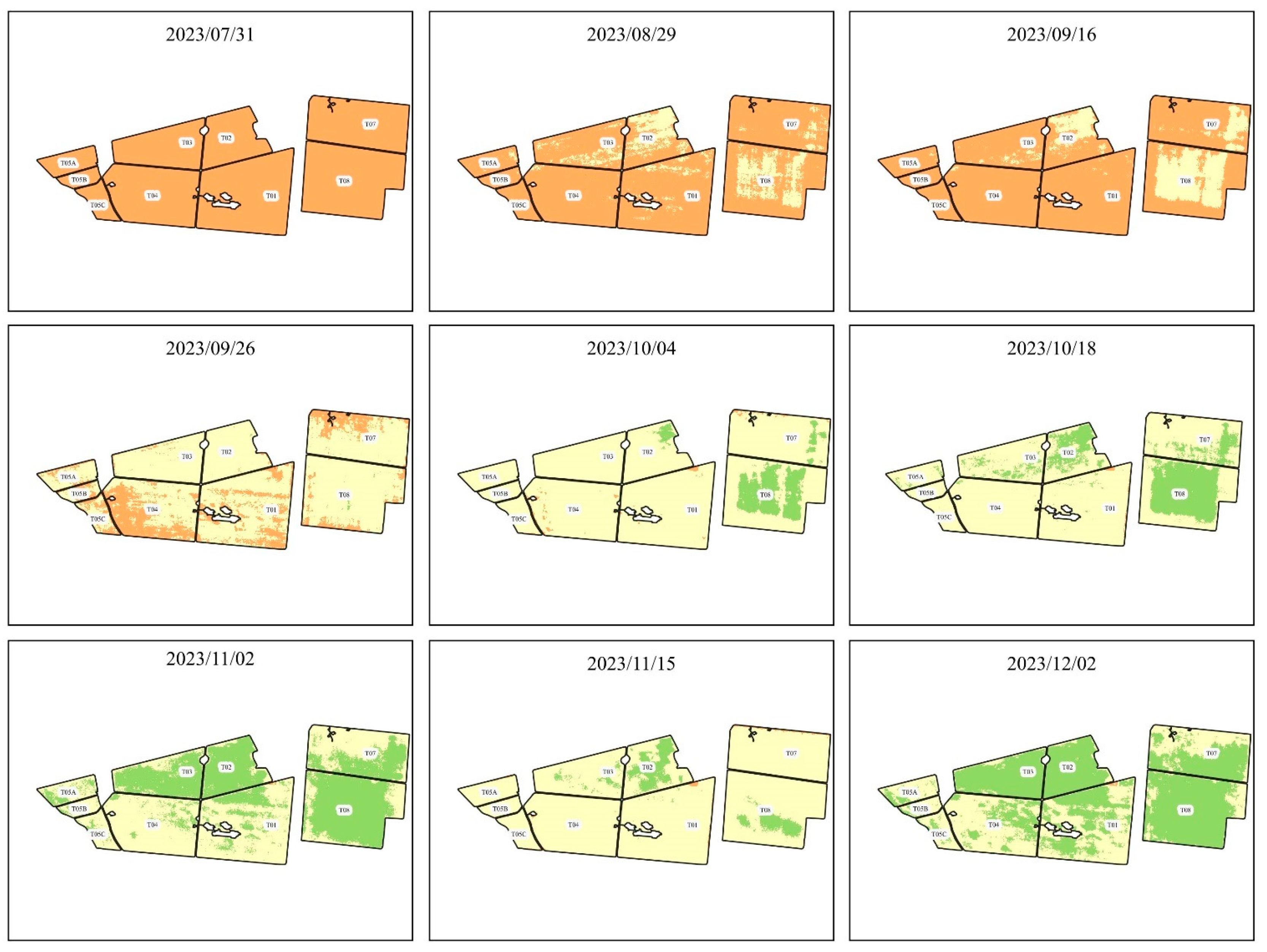
Figure 3. NDVI evolution from 2023/12/18 to 2024/02/27.

Figure 3. NDVI evolution from 2023/12/18 to 2024/02/27.

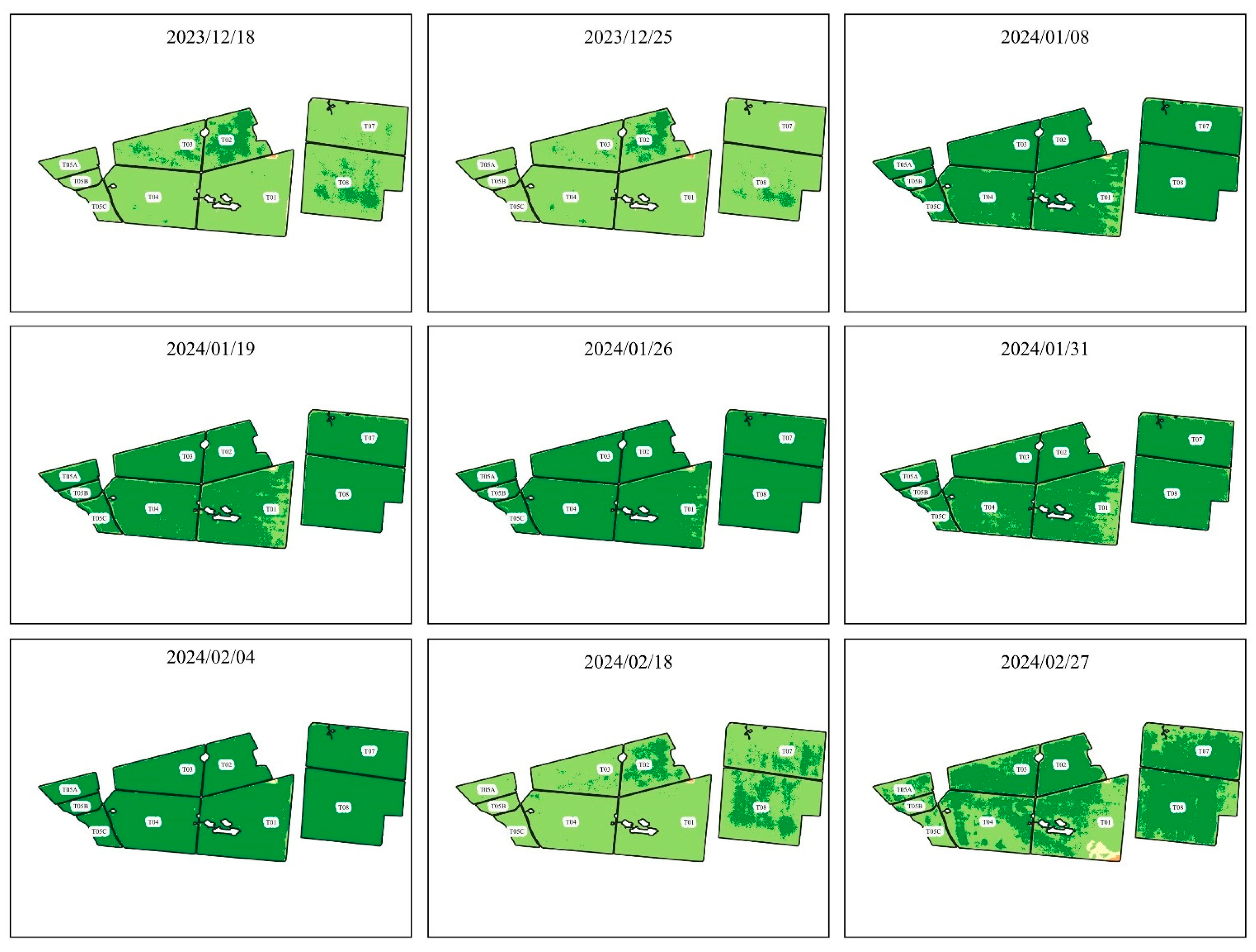
Figure 4. NDVI evolution from 2024/03/01 to 2024/05/05.

Figure 4. NDVI evolution from 2024/03/01 to 2024/05/05.

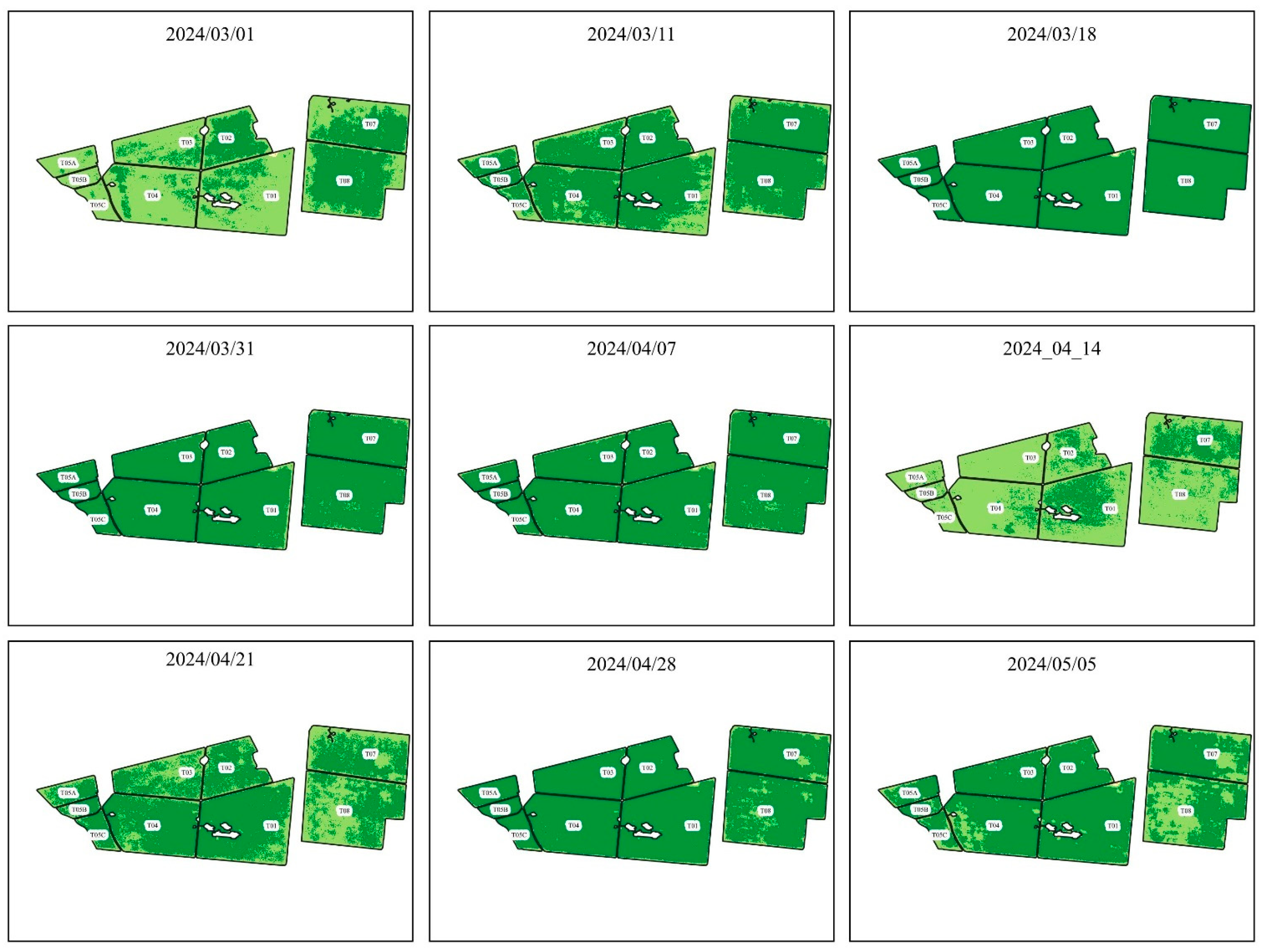
Figure 5. NDVI evolution from 2024/05/12 to 2024/06/16.

Figure 5. NDVI evolution from 2024/05/12 to 2024/06/16.

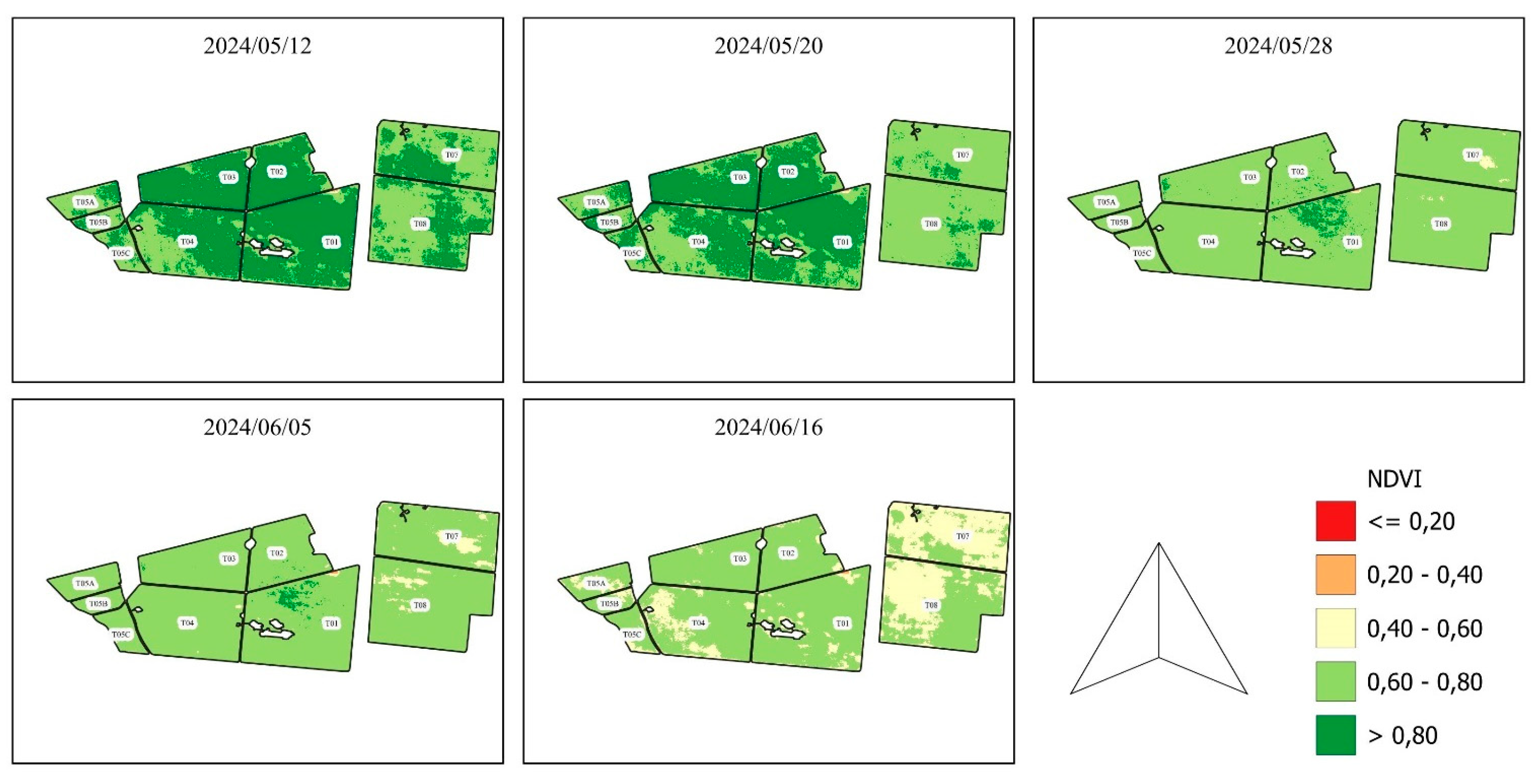
presents the NDVIs found using the images of the Planet constellation and after processing the images in QGIS.

Table 5. Mean NDVI per plot.

Date	T01	T02	T03	T04	T05A	T05B	T05C	T07	T08
06/30/2023	0.00	0.00	0.00	0.00	0.00	0.00	0.00	0.00	0.00
07/31/2023	0.31	0.32	0.31	0.31	0.32	0.31	0.31	0.29	0.31
08/29/2023	0.37	0.40	0.38	0.36	0.37	0.36	0.36	0.36	0.38
09/16/2023	0.35	0.40	0.37	0.34	0.35	0.34	0.34	0.36	0.40
09/26/2023	0.41	0.47	0.44	0.40	0.42	0.41	0.40	0.43	0.48
10/04/2023	0.48	0.54	0.51	0.47	0.50	0.49	0.48	0.51	0.56
10/18/2023	0.53	0.59	0.57	0.52	0.56	0.54	0.53	0.56	0.61
11/02/2023	0.57	0.64	0.61	0.56	0.58	0.57	0.57	0.58	0.64
11/15/2023	0.51	0.58	0.56	0.48	0.48	0.47	0.47	0.49	0.55
12/02/2023	0.59	0.66	0.64	0.58	0.57	0.57	0.57	0.60	0.64
12/18/2023	0.71	0.79	0.77	0.71	0.71	0.70	0.69	0.74	0.77
12/25/2023	0.70	0.78	0.76	0.71	0.69	0.69	0.68	0.73	0.75
01/08/2024	0.81	0.86	0.85	0.82	0.82	0.81	0.81	0.84	0.85
01/19/2024	0.81	0.84	0.84	0.82	0.82	0.82	0.81	0.83	0.83
01/26/2024	0.82	0.86	0.86	0.84	0.83	0.82	0.83	0.86	0.86
01/31/2024	0.80	0.84	0.83	0.82	0.81	0.82	0.81	0.83	0.83
02/04/2024	0.84	0.87	0.86	0.85	0.85	0.85	0.85	0.87	0.87
02/18/2024	0.75	0.78	0.77	0.73	0.74	0.73	0.71	0.77	0.78
03/01/2024	0.78	0.80	0.78	0.78	0.77	0.77	0.76	0.79	0.80
03/11/2024	0.80	0.81	0.80	0.81	0.80	0.80	0.79	0.81	0.81
03/18/2024	0.85	0.85	0.84	0.85	0.84	0.85	0.85	0.85	0.85
03/31/2024	0.82	0.83	0.82	0.83	0.83	0.83	0.83	0.82	0.82
04/07/2024	0.82	0.82	0.82	0.83	0.82	0.83	0.82	0.82	0.82
04/14/2024	0.79	0.79	0.78	0.78	0.78	0.79	0.78	0.80	0.79
04/21/2024	0.81	0.80	0.80	0.81	0.80	0.81	0.80	0.80	0.80
04/28/2024	0.83	0.83	0.83	0.83	0.83	0.83	0.83	0.82	0.81
05/05/2024	0.82	0.82	0.81	0.81	0.80	0.81	0.80	0.81	0.80
05/12/2024	0.81	0.81	0.81	0.80	0.78	0.79	0.78	0.78	0.79
05/20/2024	0.81	0.81	0.81	0.80	0.79	0.79	0.78	0.75	0.76
05/28/2024	0.76	0.77	0.77	0.74	0.74	0.74	0.73	0.70	0.71
06/05/2024	0.76	0.75	0.75	0.74	0.73	0.74	0.73	0.70	0.70
06/13/2024	0.75	0.73	0.73	0.73	0.72	0.73	0.72	0.68	0.68

Plots T01, T02, T03, and T04 received treatment. Plots T05A, T05B, T05C, T07, and T08 are control.

Table 5. Mean NDVI per plot.

Date	T01	T02	T03	T04	T05A	T05B	T05C	T07	T08
06/30/2023	0.00	0.00	0.00	0.00	0.00	0.00	0.00	0.00	0.00
07/31/2023	0.31	0.32	0.31	0.31	0.32	0.31	0.31	0.29	0.31
08/29/2023	0.37	0.40	0.38	0.36	0.37	0.36	0.36	0.36	0.38
09/16/2023	0.35	0.40	0.37	0.34	0.35	0.34	0.34	0.36	0.40
09/26/2023	0.41	0.47	0.44	0.40	0.42	0.41	0.40	0.43	0.48
10/04/2023	0.48	0.54	0.51	0.47	0.50	0.49	0.48	0.51	0.56
10/18/2023	0.53	0.59	0.57	0.52	0.56	0.54	0.53	0.56	0.61
11/02/2023	0.57	0.64	0.61	0.56	0.58	0.57	0.57	0.58	0.64
11/15/2023	0.51	0.58	0.56	0.48	0.48	0.47	0.47	0.49	0.55
12/02/2023	0.59	0.66	0.64	0.58	0.57	0.57	0.57	0.60	0.64
12/18/2023	0.71	0.79	0.77	0.71	0.71	0.70	0.69	0.74	0.77
12/25/2023	0.70	0.78	0.76	0.71	0.69	0.69	0.68	0.73	0.75
01/08/2024	0.81	0.86	0.85	0.82	0.82	0.81	0.81	0.84	0.85
01/19/2024	0.81	0.84	0.84	0.82	0.82	0.82	0.81	0.83	0.83
01/26/2024	0.82	0.86	0.86	0.84	0.83	0.82	0.83	0.86	0.86
01/31/2024	0.80	0.84	0.83	0.82	0.81	0.82	0.81	0.83	0.83
02/04/2024	0.84	0.87	0.86	0.85	0.85	0.85	0.85	0.87	0.87
02/18/2024	0.75	0.78	0.77	0.73	0.74	0.73	0.71	0.77	0.78
03/01/2024	0.78	0.80	0.78	0.78	0.77	0.77	0.76	0.79	0.80
03/11/2024	0.80	0.81	0.80	0.81	0.80	0.80	0.79	0.81	0.81
03/18/2024	0.85	0.85	0.84	0.85	0.84	0.85	0.85	0.85	0.85
03/31/2024	0.82	0.83	0.82	0.83	0.83	0.83	0.83	0.82	0.82
04/07/2024	0.82	0.82	0.82	0.83	0.82	0.83	0.82	0.82	0.82
04/14/2024	0.79	0.79	0.78	0.78	0.78	0.79	0.78	0.80	0.79
04/21/2024	0.81	0.80	0.80	0.81	0.80	0.81	0.80	0.80	0.80
04/28/2024	0.83	0.83	0.83	0.83	0.83	0.83	0.83	0.82	0.81
05/05/2024	0.82	0.82	0.81	0.81	0.80	0.81	0.80	0.81	0.80
05/12/2024	0.81	0.81	0.81	0.80	0.78	0.79	0.78	0.78	0.79
05/20/2024	0.81	0.81	0.81	0.80	0.79	0.79	0.78	0.75	0.76
05/28/2024	0.76	0.77	0.77	0.74	0.74	0.74	0.73	0.70	0.71
06/05/2024	0.76	0.75	0.75	0.74	0.73	0.74	0.73	0.70	0.70
06/13/2024	0.75	0.73	0.73	0.73	0.72	0.73	0.72	0.68	0.68

Plots T01, T02, T03, and T04 received treatment. Plots T05A, T05B, T05C, T07, and T08 are control.

Using the Real Statistic tool, it was possible to obtain the second-order polynomial regression curves - - as well as the values of R² and coefficients a, b, and c - .

Figure 6. NDVI dispersion and second-order polynomial regression.

Figure 6. NDVI dispersion and second-order polynomial regression.

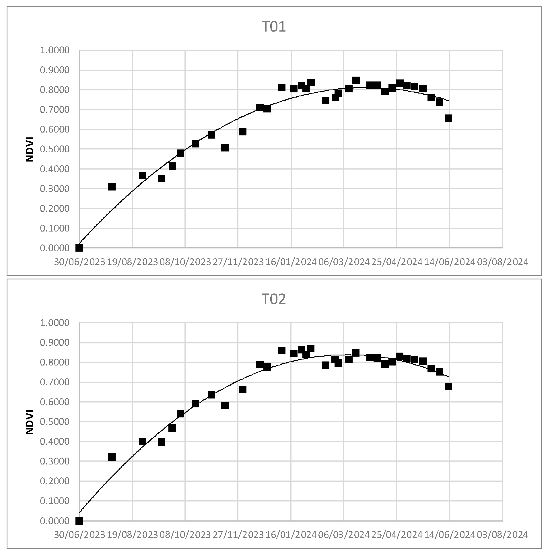
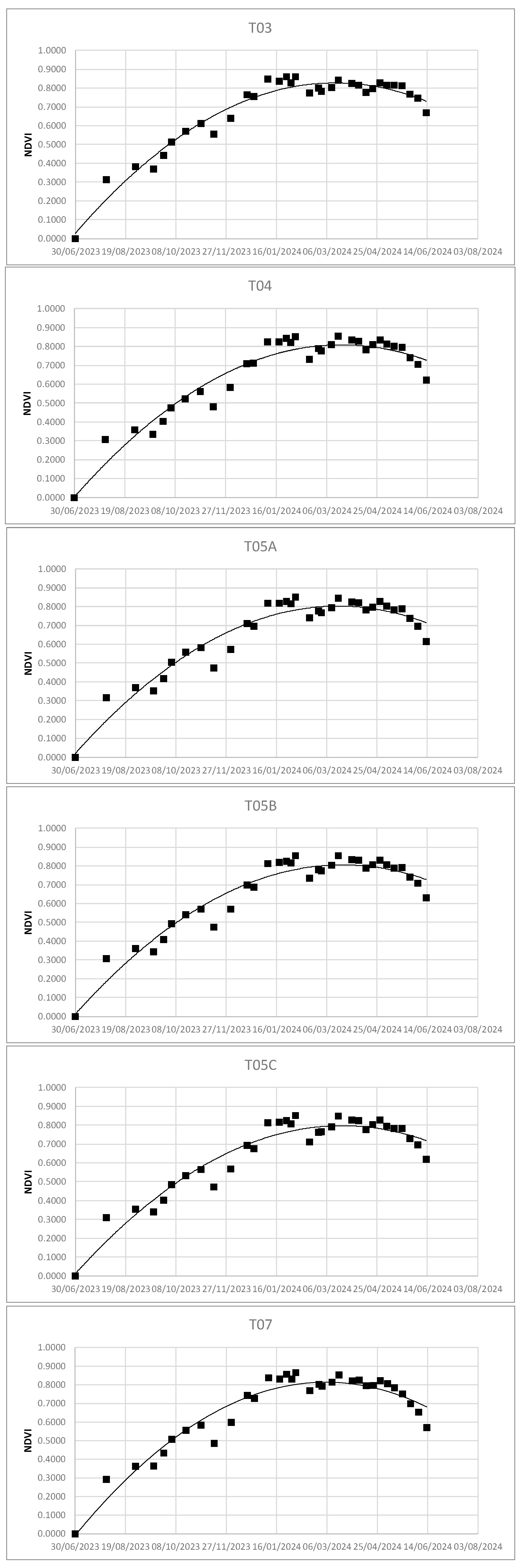
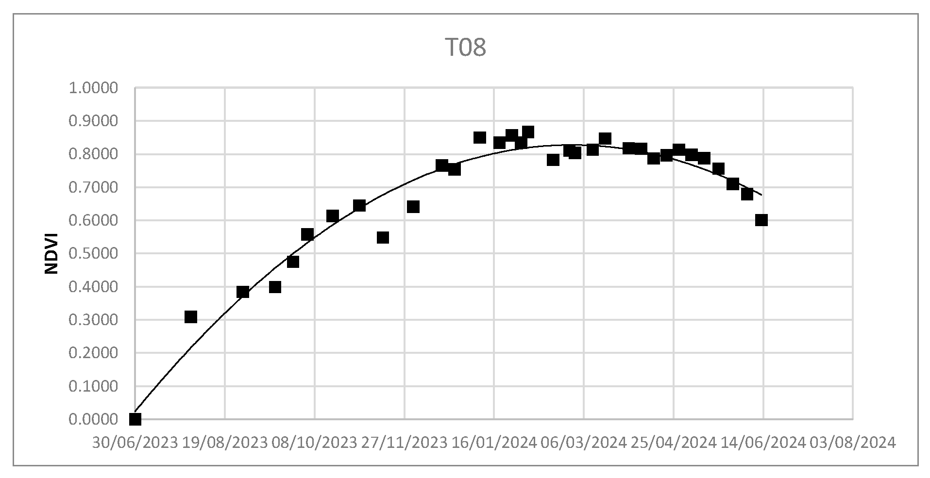
Table 6. Pearson’s coefficient of determination (R2) and coefficients a, b, and c for second-order polynomial regression curves.

Parameter	T01	T02	T03	T04	T05A	T05B	T05C	T07	T08
R2	0.946	0.959	0.952	0.927	0.924	0.929	0.921	0.927	0.950
a	-0.00001067	-0.00001235	-0.00001190	-0.00001146	-0.00001141	-0.00001118	-0.00001111	-0.00001321	-0.00001348
b	0.00580970	0.00629514	0.00618118	0.00609320	0.00599155	0.00596708	0.00591800	0.00660758	0.00659663
c	0.01928293	0.03672080	0.02491970	-0.00136835	0.01625712	0.00844668	0.00817122	-0.01279157	0.02008156

Table 6. Pearson’s coefficient of determination (R2) and coefficients a, b, and c for second-order polynomial regression curves.

Parameter	T01	T02	T03	T04	T05A	T05B	T05C	T07	T08
R2	0.946	0.959	0.952	0.927	0.924	0.929	0.921	0.927	0.950
a	-0.00001067	-0.00001235	-0.00001190	-0.00001146	-0.00001141	-0.00001118	-0.00001111	-0.00001321	-0.00001348
b	0.00580970	0.00629514	0.00618118	0.00609320	0.00599155	0.00596708	0.00591800	0.00660758	0.00659663
c	0.01928293	0.03672080	0.02491970	-0.00136835	0.01625712	0.00844668	0.00817122	-0.01279157	0.02008156

The values of R² observed in indicate that in the worst scenario (T05C), 92.1% of the variability of the dependent variable is explained by the model, while the remaining 7.9% is due to other variables not included in the model or to random error. This being said, progress was made in the stages of integration of the equations obtained and VAI.

presents the VAI values for the total period of plant development, which goes from June 30, 2023 to May 28, 2024, and for the post-treatment period of the tested product, from February 5, 2024 to May 28, 2024.

Table 7. Vegetation Activity Index (VAI).

Plot	Condition	VAI 06/30/2023 to 05/28/2024	VAI 02/05/2024 to 05/28/2024
T01	Treated	210.12	103.15
T02	Treated	221.91	105.33
T03	Treated	217.21	104.39
T04	Treated	208.92	102.45
T05A	Control	209.54	101.48
T05B	Control	208.72	102.13
T05C	Control	206.56	100.98
T07	Control	211.48	101.27
T08	Control	218.39	102.19

Table 7. Vegetation Activity Index (VAI).

Plot	Condition	VAI 06/30/2023 to 05/28/2024	VAI 02/05/2024 to 05/28/2024
T01	Treated	210.12	103.15
T02	Treated	221.91	105.33
T03	Treated	217.21	104.39
T04	Treated	208.92	102.45
T05A	Control	209.54	101.48
T05B	Control	208.72	102.13
T05C	Control	206.56	100.98
T07	Control	211.48	101.27
T08	Control	218.39	102.19

From , the normality test was performed using the Shapiro-Wilk test - - and QQ plot for the Treated and Control groups, considering the total period - - and the post-treatment period - .

Table 8. Shapiro-Wilk Test for VAI for total and post-treatment period.

	Total period		Post-treatment period
	Treated	Control	Treated	Control
W-stat	0.91	0.89	0.97	0.90
p-value	0.48	0.35	0.84	0.42
Alpha	0.05	0.05	0.05	0.05
Normal	yes	yes	yes	yes

Table 8. Shapiro-Wilk Test for VAI for total and post-treatment period.

	Total period		Post-treatment period
	Treated	Control	Treated	Control
W-stat	0.91	0.89	0.97	0.90
p-value	0.48	0.35	0.84	0.42
Alpha	0.05	0.05	0.05	0.05
Normal	yes	yes	yes	yes

Evaluating the total period for both groups, the W-stat values (0.91 and 0.89) suggest that the data are close to a normal distribution. The p-values (0.48 for Treated and 0.35 for Control) are both higher than the 0.05significance level. The data of both groups are normally distributed.

The W-stat values (0.97 and 0.90) for the post-treatment period suggest that the data are close to a normal distribution. The p-values (0.84 for Treated and 0.42 for Control) are both higher than the 0.05 significance level. We conclude that the data of both groups are normally distributed.

Figure 7. VAI QQ plot for total period for Treated group (A) and Control group (B).

Figure 7. VAI QQ plot for total period for Treated group (A) and Control group (B).

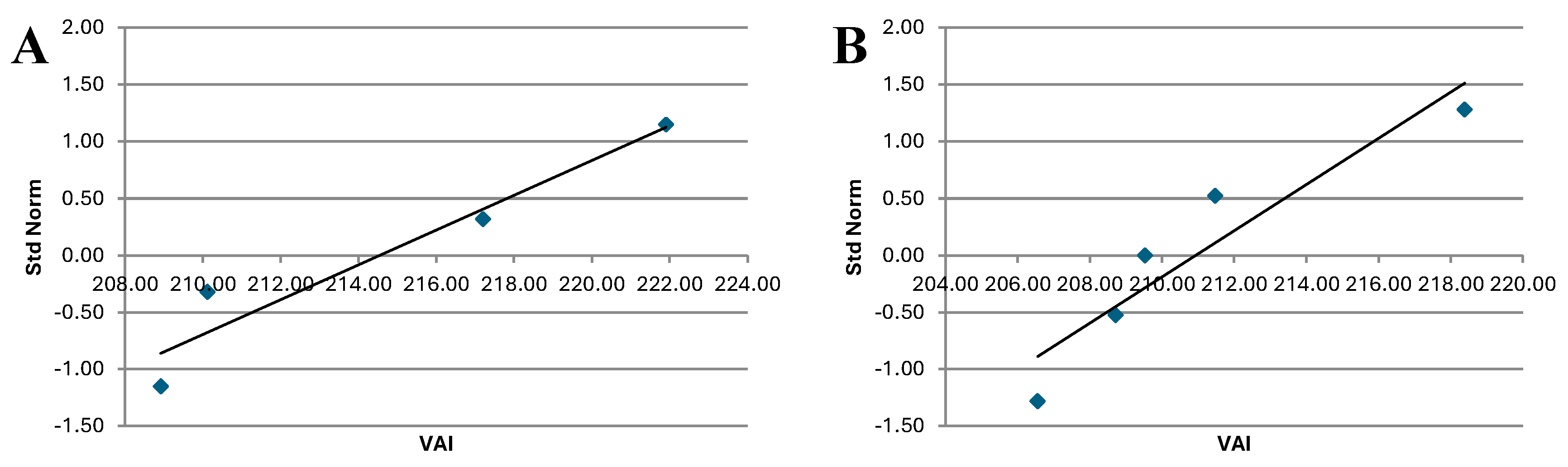
The analysis of indicates that the QQ plot of both Treated and Control groups follows a distribution that approximates a normal one. This is consistent with the results of the Shapiro-Wilk Test, which also suggest normality of the data.

Figure 8. VAI QQ plot for post-treatment period for Treated group (A) and Control group (B).

Figure 8. VAI QQ plot for post-treatment period for Treated group (A) and Control group (B).

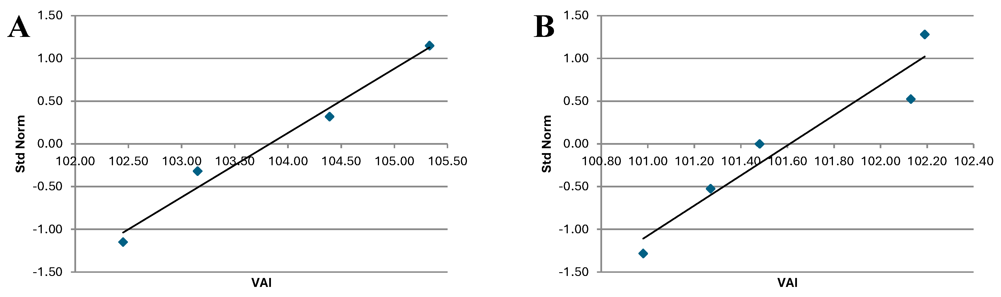
The analysis of indicates that the QQ plot of both Treated and Control groups follows a distribution that approximates a normal one. This is consistent with the results of the Shapiro-Wilk Test, which also suggest normality of the data.

Validating the normality of the data and using the data presented in , the t-test was performed in two samples assuming equivalent variances -.

Table 9. VAI t-test: two samples assuming equivalent variances for total period.

	Total period		Post-treatment period
	Treated	Control	Treated	Control
Mean	214.54	210.94	103.83	101.61
Variance	37.522	20.467	1.643	0.284
Observations	4	5	4	5
Clustered variance	27.776		0.867
Mean difference hypothesis	0.000		0.000
gl	7.000		7.000
Stat t	1.019		3.555
P(T<=t) one-tailed	0.171		0.005
critical t one-tailed	1.895		1.895
P(T<=t) two-tailed	0.342		0.009
critical t two-tailed	2.365		2.365

Table 9. VAI t-test: two samples assuming equivalent variances for total period.

	Total period		Post-treatment period
	Treated	Control	Treated	Control
Mean	214.54	210.94	103.83	101.61
Variance	37.522	20.467	1.643	0.284
Observations	4	5	4	5
Clustered variance	27.776		0.867
Mean difference hypothesis	0.000		0.000
gl	7.000		7.000
Stat t	1.019		3.555
P(T<=t) one-tailed	0.171		0.005
critical t one-tailed	1.895		1.895
P(T<=t) two-tailed	0.342		0.009
critical t two-tailed	2.365		2.365

Evaluating the total period, the results of the t-test for two samples, assuming equivalent variances, show that the mean of the Treated group (214.54) is higher than the mean of the Control group (210.938). The variance of the data in the Treated group is higher (37.522) compared to the Control group (20.467), indicating greater dispersion in the Treated group.

The calculated t-statistic is 1.019. The p-value for the one-tailed test is 0.171, and for the two-tailed test is 0.342, both higher than the 0.05 significance level. Therefore, no statistically significant difference was found between the means of the two samples, with 95% confidence.

For the post-treatment period, the results of the t-test for two samples, assuming equivalent variances, show that the mean of the Treated group (103.83) is higher than the mean of the Control group (101.61). The variance of the data in the Treated group is higher (1.643) compared to the Control group (0.284), indicating greater dispersion in the Treated group. The VAI for the Treated group was 2.18% higher than that of the Control group, a result below those found by Chen et al. (2021) and Raju et al. (2022).

The calculated t-statistic is 3.5549. The p-value for the one-tailed test is 0.0046, and for the two-tailed test is 0.0093, both lower than the 0.05 significance level. This leads us to reject the null hypothesis that there is no difference between the means of the groups. Therefore, we conclude that the mean of the Treated group is significantly higher than that of the Control group, with 95% confidence.

After the plots were harvested, the data found were presented in .

Table 10. Post-harvest results from the area under study.

Plots	Area	SCTH	Production	F	Pza	PCC	RS	SRS	TRS	STH
Treated
01	34.06	94.73	3.226,50	11.92	86.33	13.83	0.58	15.14	138.53	13.12
02	15.20	106.36	1.616,67	12.29	85.91	13.54	0.58	14.83	135.69	14.43
03	17.72	103.12	1.827,29	11.57	89.76	13.88	0.48	15.09	138.07	14.24
04	26.41	90.46	2.389,05	12.00	87.29	14.41	0.55	15.72	143.84	13.01
Total treated	93.39	97.01	9.059,51	11.94	87.20	13.94	0.55	15.23	139.35	13.52
Control
05th	6.00	94.92	569.52	12.25	86.65	14.47	0.56	15.79	144.48	13.71
05B	3.05	95.52	291.34	12.33	87.21	14.57	0.56	15.90	145.49	13.90
05C	4.74	94.45	447.69	12.19	86.23	14.40	0.56	15.72	143.84	13.59
07	28.87	94.78	2.736,30	12.16	85.10	13.12	0.61	14.42	131.94	12.51
08	33.96	102.15	3.469,01	12.13	86.67	12.94	0.56	14.18	129.75	13.25
Total control	76.62	98.07	7.513,86	12.16	86.09	13.27	0.58	14.55	133.13	13.06

Table 10. Post-harvest results from the area under study.

Plots	Area	SCTH	Production	F	Pza	PCC	RS	SRS	TRS	STH
Treated
01	34.06	94.73	3.226,50	11.92	86.33	13.83	0.58	15.14	138.53	13.12
02	15.20	106.36	1.616,67	12.29	85.91	13.54	0.58	14.83	135.69	14.43
03	17.72	103.12	1.827,29	11.57	89.76	13.88	0.48	15.09	138.07	14.24
04	26.41	90.46	2.389,05	12.00	87.29	14.41	0.55	15.72	143.84	13.01
Total treated	93.39	97.01	9.059,51	11.94	87.20	13.94	0.55	15.23	139.35	13.52
Control
05th	6.00	94.92	569.52	12.25	86.65	14.47	0.56	15.79	144.48	13.71
05B	3.05	95.52	291.34	12.33	87.21	14.57	0.56	15.90	145.49	13.90
05C	4.74	94.45	447.69	12.19	86.23	14.40	0.56	15.72	143.84	13.59
07	28.87	94.78	2.736,30	12.16	85.10	13.12	0.61	14.42	131.94	12.51
08	33.96	102.15	3.469,01	12.13	86.67	12.94	0.56	14.18	129.75	13.25
Total control	76.62	98.07	7.513,86	12.16	86.09	13.27	0.58	14.55	133.13	13.06

It is assumed that the amino acid L-alpha acts in the metabolism of plants, contributing to various physiological processes that affect growth and development, especially in protein synthesis and stress response. Under stress conditions, plants treated with L-alpha tend to maintain or improve the quality of sugars, even though productivity in terms of biomass may be affected.

Thus, it was decided to evaluate its impact on sugarcane by a comprehensive indicator such as STH (sugar tons per hectare). This indicator captures not only productivity in terms of SCTH (sugarcane tons per hectare), but also sugarcane quality in terms of sugar content (TRS - total recoverable sugars), providing a more comprehensive view of plant performance under the influence of the amino acid L-alpha.

From , the normality test was performed using the Shapiro-Wilk Test - - and QQ plot for Treated and Control groups - .

Table 11. Shapiro-Wilk Test for post-harvest STH.

	Treated	Control
W-stat	0.83	0.89
p-value	0.16	0.37
alpha	0.05	0.05
normal	yes	yes

Table 11. Shapiro-Wilk Test for post-harvest STH.

	Treated	Control
W-stat	0.83	0.89
p-value	0.16	0.37
alpha	0.05	0.05
normal	yes	yes

For both groups, the W-stat values (0.83 and 0.89) suggest that the data are close to a normal distribution. The p-values (0.16 for Treated and 0.37 for Control) are both higher than the 0.05 significance level. The data of both groups are normally distributed.

Figure 9. STH QQ plot for post-treatment period for Treated group (A) and Control group (B).

Figure 9. STH QQ plot for post-treatment period for Treated group (A) and Control group (B).

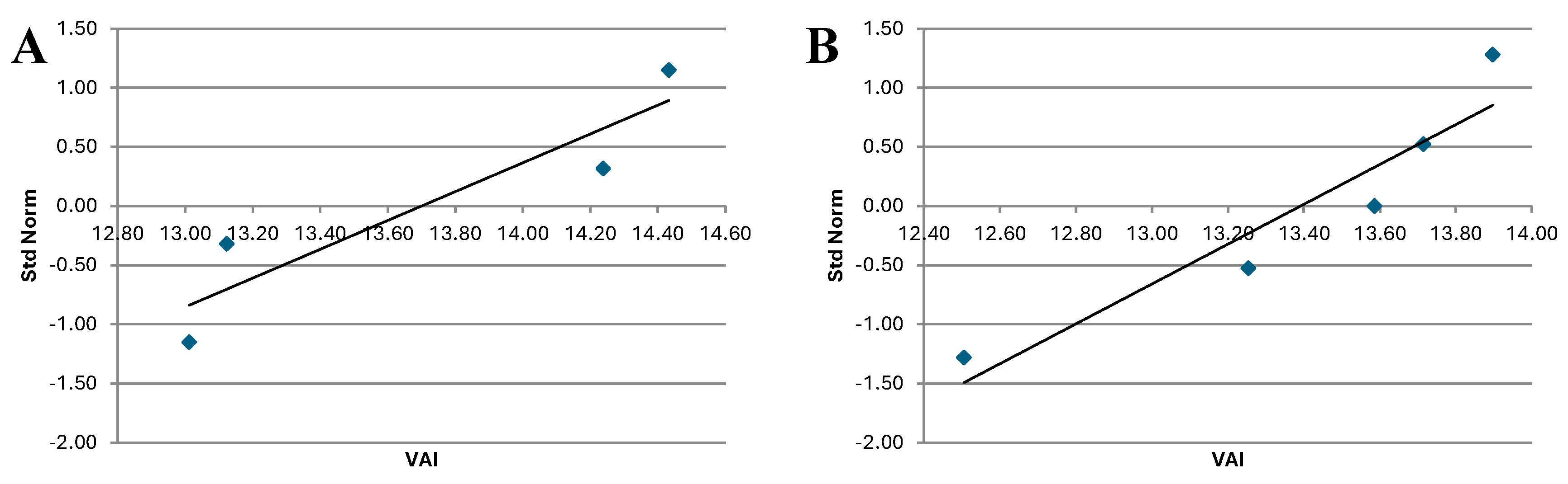
The analysis of indicates that the QQ plot of both Treated and Control groups follows a distribution that approximates a normal one. This is consistent with the results of the Shapiro-Wilk Test, which also suggest normality of the data.

As there is normality in STH for both Treated and Control group, the two-sample t-test was performed assuming equivalent variances for the assessment of STH in both groups - .

Table 12. STH t-test: two samples assuming equivalent variances for post-harvest period.

	Treated	Control
Mean	13.70	13.39
Variance	0.552	0.299
Observations	4	5
Clustered variance	0.407
Mean difference hypothesis	0.000
gl	7.000
Stat t	0.724
P(T<=t) one-tailed	0.246
critical t one-tailed	1.895
P(T<=t) two-tailed	0.492
critical t two-tailed	2.365

Table 12. STH t-test: two samples assuming equivalent variances for post-harvest period.

	Treated	Control
Mean	13.70	13.39
Variance	0.552	0.299
Observations	4	5
Clustered variance	0.407
Mean difference hypothesis	0.000
gl	7.000
Stat t	0.724
P(T<=t) one-tailed	0.246
critical t one-tailed	1.895
P(T<=t) two-tailed	0.492
critical t two-tailed	2.365

The results of the t-test for two samples, assuming equivalent variances, presented in , show that the mean of the Treated group (13.70) is higher than the mean of the Control group (13.29). The variance of the data in the Treated group is higher (0.552) compared to the Control group (0.298), indicating greater dispersion in the Treated group.

The calculated t-statistic is 0.724. The p-value for the one-tailed test is 0.246, and for the two-tailed test is 0.492, both higher than the 0.05 significance level. Therefore, no statistically significant difference was found between the means of the two samples, with 95% confidence. Comparing the means, there is a gain of 2.32% in STH, a value below that observed by Chen et al. (2021), who showed gains from 3.33 to 9.23% in productivity and 5.00% increase in sucrose, and Jacomassi et al. (2022), who found an increase in sugars per hectare of 3.4 kg Mg^-1.

The final stage of the statistical analysis was the verification of the correlation between the variables post-harvest VAI and STH. The results obtained are presented in .

Table 13. Pearson’s correlation between VAI and STH for the Treated and Control groups.

	Treated	Control
Alpha	0.050	0.050
Tails	2	2.0
corr	0.966	0.274
std err	0.182	0.555
t	5.325	0.494
p-value	0.034	0.655
lower	0.186	-1.493
upper	1.747	2.041

Table 13. Pearson’s correlation between VAI and STH for the Treated and Control groups.

	Treated	Control
Alpha	0.050	0.050
Tails	2	2.0
corr	0.966	0.274
std err	0.182	0.555
t	5.325	0.494
p-value	0.034	0.655
lower	0.186	-1.493
upper	1.747	2.041

For the Treated group, the coefficient of correlation (r) was 0.966, indicating a very strong positive correlation between VAI and STH. The p-value of 0.034 is less than 0.05, which suggests that the observed correlation is statistically significant. The 95% confidence interval for the coefficient of correlation is between 0.186 and 1.747, which indicates a high probability that the true value of the coefficient of correlation is within this range.

For the Control group, the coefficient of correlation (r) was 0.274, indicating a milder positive correlation between VAI and STH. The p-value of 0.655 is greater than 0.05, indicating that the observed correlation is not statistically significant, with a 95% confidence level. The wide confidence interval (-1.493 to 2.041) suggests considerable uncertainty regarding the true value of the coefficient of correlation in this area, indicating that the correlation may vary substantially.

The return on investment assessment is presented in from the parameters established for agroindustrial modeling - - and the post-harvest results of the area under study - .

Table 14. Economic feasibility analysis.

Variables	Control	Treatment	Difference
SCTH	98.07	97.01	-1.06
CHar	11.17	11.29	0.12
CTrac	11.09	11.12	0.03
CTransp	16.18	16.18	0.00
CTT	3.769,05	3.743,51	-25.53
CProc	2.770,38	2.740,46	-29.93
CTrat		165.00	165.00
CTot	6.539,43	6.648,97	109.54
F	12.16	11.94	-0.22
Pza	86.09	87.20	1.11
PCC	13.27	13.94	0.67
RS	0.58	0.55	-0.03
SRS	14.55	15.23	0.68
TRS	133.13	139.35	6.22
STH	13.06	13.52	0.46
R_SJM	88.47	89.48	1.01
Sugar	108.34	113.87	5.52
Ethanol	4.339,45	4.439,05	99.61
AEC	1.860,95	1.903,66	42.72
HEC	2.606,12	2.665,94	59.82
Energy	6.57	6.50	-0.07
GR	26.814,74	27.816,77	1.002,03
NR	20.275,31	21.167,80	892.49
ROI			541%

Table 14. Economic feasibility analysis.

Variables	Control	Treatment	Difference
SCTH	98.07	97.01	-1.06
CHar	11.17	11.29	0.12
CTrac	11.09	11.12	0.03
CTransp	16.18	16.18	0.00
CTT	3.769,05	3.743,51	-25.53
CProc	2.770,38	2.740,46	-29.93
CTrat		165.00	165.00
CTot	6.539,43	6.648,97	109.54
F	12.16	11.94	-0.22
Pza	86.09	87.20	1.11
PCC	13.27	13.94	0.67
RS	0.58	0.55	-0.03
SRS	14.55	15.23	0.68
TRS	133.13	139.35	6.22
STH	13.06	13.52	0.46
R_SJM	88.47	89.48	1.01
Sugar	108.34	113.87	5.52
Ethanol	4.339,45	4.439,05	99.61
AEC	1.860,95	1.903,66	42.72
HEC	2.606,12	2.665,94	59.82
Energy	6.57	6.50	-0.07
GR	26.814,74	27.816,77	1.002,03
NR	20.275,31	21.167,80	892.49
ROI			541%

The ROI obtained indicates that for each monetary unit invested, 5.41 units will be returned, indicating the high profitability of the treatment.

4. Conclusions

This study analyzed the impact of treatment with L-alpha amino acid on sugarcane, using the vegetation activity index (VAI) and the post-harvest productivity and quality metrics. The VAI results, obtained from NDVI images processed in QGIS, showed significant variations over time between the treated and control areas.

Normality tests, both by the Shapiro-Wilk method and by QQ plots, confirmed that VAI and STH data for both groups, treated and control, follow a normal distribution. Statistical analysis, including the t-test for independent samples, revealed that:

For the VAI of the total period of plant development (06/30/2023 to 05/28/2024), no statistically significant difference was found between the treated and control groups. The p-value obtained was 0.084, which is higher than 0.05, indicating no statistical significance. This suggests that the treatment did not have a significant impact on the overall development of vegetation during the entire cycle.

In the post-treatment period (02/05/2024 to 05/28/2024), the results indicated a statistically significant difference between the groups. The p-value was 0.021, which is lower than 0.05, with the treated group presenting a higher VAI than the control group. This finding suggests that the treatment had a significant positive effect on plant activity during this specific period.

In the post-harvest analysis, the results of the t-test indicated no statistically significant difference between the STH of the treated areas and the control areas. The calculated t value was 1.354, which is lower than the critical t value (2.042 for the two-tailed test and 1.782 for the one-tailed test). This suggests that L-alpha treatment did not have a significant impact on the amount of recoverable sugars per hectare compared to the untreated area.

The coefficients of determination (R²) of the polynomial regressions indicated that the models explain well the variability of the NDVI data, with values ranging from 0.921 to 0.959. These high R² values reinforce the robustness of the models applied to understand vegetation dynamics.

The results found show that the use of L-alpha can be an effective strategy to increase plant activity during critical periods of sugarcane development, as indicated by the results of VAI in the post-treatment period. However, no significant impact on sugar productivity per hectare was observed.

ROI analysis shows that, for each monetary unit invested, 5.41 units will be returned, indicating the high profitability of the treatment.

The inclusion of a larger number of samples could allow a more detailed exploration of the results, especially for post-harvest data. A larger sample size can increase the accuracy of estimates, reducing the margin of error and providing a more comprehensive understanding of treatment effects. With a larger volume of samples, it would also be possible to evaluate the correlation between VAI and STH in a more robust way, identifying possible relationships between plant activity during the cycle and the final productivity of sugars per hectare.

We recommended continued research in this area, with a larger number of samples, in different environmental conditions, and with different varieties of sugarcane, to validate and expand the findings obtained in this study.

References

- Akbarian, S., Xu, C. Y., & Lim, S. (2020). Analysis on the effect of spatial and spectral resolution of different remote sensing data in sugarcane crop yield study. ISPRS Annals of the Photogrammetry, Remote Sensing and Spatial Information Sciences, 5(3), 655-661. [CrossRef]
- Akbarian, S., Xu, C., Wang, W., Ginns, S., & Lim, S. (2022). Sugarcane yields prediction at the row level using a novel cross-validation approach to multi-year multispectral images. Computers and Electronics in Agriculture, 198, 107024. [CrossRef]
- Ali, O., Ramsubhag, A., & Jayaraman, J. (2021). Biostimulant properties of seaweed extracts in plants: Implications towards sustainable crop production. Plants, 10(3), 531. [CrossRef]
- Ashraf, M., & Foolad, M. R. (2007). Roles of glycine betaine and proline in improving plant abiotic stress resistance. Environmental and experimental botany, 59(2), 206-216. [CrossRef]
- Bramley, R. G. V., Ouzman, J., & Gobbett, D. L. (2019). Regional scale application of the precision agriculture thought process to promote improved fertilizer management in the Australian sugar industry. Precision Agriculture, 20, 362-378. [CrossRef]
- Calvo, P., Nelson, L., & Kloepper, J. W. (2014). Agricultural uses of plant biostimulants. Plant and soil, 383(1-2), 3-41. [CrossRef]
- Canata, T. F., Wei, M. C. F., Maldaner, L. F., & Molin, J. P. (2021). Sugarcane yield mapping using high-resolution imagery data and machine learning technique. Remote Sensing, 13(2), 232. [CrossRef]
- Carreño-Conde, F., Sipols, A. E., de Blas, C. S., & Mostaza-Colado, D. (2021). A forecast model applied to monitor crops dynamics using vegetation indices (Ndvi). Applied Sciences, 11(4), 1859. [CrossRef]
- Calicioglu, O., Flammini, A., Bracco, S., Bellù, L., & Sims, R. (2019). The future challenges of food and agriculture: An integrated analysis of trends and solutions. Sustainability, 11(1), 222. [CrossRef]
- Chen, D., Zhou, W., Yang, J., Ao, J., Huang, Y., Shen, D., ... & Shen, H. (2021). Effects of seaweed extracts on the growth, physiological activity, cane yield and sucrose content of sugarcane in China. Frontiers in Plant Science, 12, 659130. [CrossRef]
- Dias Neto, A. F., Albiero, D., Rossetto, R., & Biagi, J. D. (2023). Management of mechanized harvesting through operational modeling. Revista Ciência Agronômica, 54, e20218193. [CrossRef]
- Dimov, D., Uhl, J. H., Löw, F., & Seboka, G. N. (2022). Sugarcane yield estimation through remote sensing time series and phenology metrics. Smart Agricultural Technology, 2, 100046. [CrossRef]
- Ding, Y., He, X., Zhou, Z., Hu, J., Cai, H., Wang, X., ... & Shi, H. (2022). Response of vegetation to drought and yield monitoring based on NDVI and SIF. Catena, 219, 106328. [CrossRef]
- Diniz, A. L., da Silva, D. I. R., Lembke, C. G., Costa, M. D. B. L., Ten-Caten, F., Li, F., ... & Souza, G. M. (2020). Amino acid and carbohydrate metabolism are coordinated to maintain energetic balance during drought in sugarcane. International Journal of Molecular Sciences, 21(23), 9124. [CrossRef]
- dos Santos Luciano, A. C., Picoli, M. C. A., Duft, D. G., Rocha, J. V., Leal, M. R. L. V., & Le Maire, G. (2021). Empirical model for forecasting sugarcane yield on a local scale in Brazil using Landsat imagery and random forest algorithm. Computers and Electronics in Agriculture, 184, 106063. [CrossRef]
- Du Jardin, P. (2015). Plant biostimulants: Definition, concept, main categories and regulation. Scientia horticulturae, 196, 3-14. [CrossRef]
- Farias, G. D., Bremm, C., Bredemeier, C., de Lima Menezes, J., Alves, L. A., Tiecher, T., ... & de Faccio Carvalho, P. C. (2023). Normalized Difference Vegetation Index (NDVI) for soybean biomass and nutrient uptake estimation in response to production systems and fertilization strategies. Frontiers in Sustainable Food Systems, 6, 959681. [CrossRef]
- Hasanuzzaman, M., Nahar, K., Alam, M. M., Roychowdhury, R., & Fujita, M. (2013). Physiological, biochemical, and molecular mechanisms of heat stress tolerance in plants. International journal of molecular sciences, 14(5), 9643-9684. [CrossRef]
- Jacomassi, L. M., Viveiros, J. D. O., Oliveira, M. P., Momesso, L., de Siqueira, G. F., & Crusciol, C. A. C. (2022). A seaweed extract-based biostimulant mitigates drought stress in sugarcane. Frontiers in Plant Science, 13, 865291. [CrossRef]
- Jeffries, G. R., Griffin, T. S., Fleisher, D. H., Naumova, E. N., Koch, M., & Wardlow, B. D. (2020). Mapping sub-field maize yields in Nebraska, USA by combining remote sensing imagery, crop simulation models, and machine learning. Precision Agriculture, 21, 678-694. [CrossRef]
- Jiang, H., Xu, X., Guan, M., Wang, L., Huang, Y., & Jiang, Y. (2020). Determining the contributions of climate change and human activities to vegetation dynamics in agro-pastural transitional zone of northern China from 2000 to 2015. Science of the Total Environment, 718, 134871. [CrossRef]
- Jin, H., Chen, X., Wang, Y., Zhong, R., Zhao, T., Liu, Z., & Tu, X. (2021). Spatio-temporal distribution of NDVI and its influencing factors in China. Journal of Hydrology, 603, 127129. [CrossRef]
- Liang, L., Wang, Q., Guan, Q., Du, Q., Sun, Y., Ni, F., ... & Shan, Y. (2023). Assessing vegetation restoration prospects under different environmental elements in cold and arid mountainous region of China. Catena, 226, 107055. [CrossRef]
- Momin, M. A., Grift, T. E., Valente, D. S., & Hansen, A. C. (2019). Sugarcane yield mapping based on vehicle tracking. Precision agriculture, 20, 896-910. [CrossRef]
- Panek, E., & Gozdowski, D. (2021). Relationship between MODIS derived NDVI and yield of cereals for selected European countries. Agronomy, 11(2), 340. [CrossRef]
- Pieterse, C. M., Zamioudis, C., Berendsen, R. L., Weller, D. M., Van Wees, S. C., & Bakker, P. A. (2014). Induced systemic resistance by beneficial microbes. Annual review of phytopathology, 52, 347-375. [CrossRef]
- Poudyal, C., Sandhu, H., Ampatzidis, Y., Odero, D. C., Arbelo, O. C., Cherry, R. H., & Costa, L. F. (2023). Prediction of morpho-physiological traits in sugarcane using aerial imagery and machine learning. Smart Agricultural Technology, 3, 100104. [CrossRef]
- Pretty, J., Benton, T. G., Bharucha, Z. P., Dicks, L. V., Flora, C. B., Godfray, H. C. J., ... & Wratten, S. (2018). Global assessment of agricultural system redesign for sustainable intensification. Nature Sustainability, 1(8), 441-446. [CrossRef]
- Rojo Baio, F. H., Neves, D. C., & Teodoro, P. E. (2019). Soil chemical attributes, soil type, and rainfall effects on normalized difference vegetation index and cotton fiber yield variability. Agronomy Journal, 111(6), 2910-2919. [CrossRef]
- Raju, G., Sailaja, N. S., Krishnapriya, V., & Prakash, M. (2022). Ameliorating drought stress in sugarcane (Saccharum spp.) using biostimulants. Indian Journal of Experimental Biology (IJEB), 60(07), 456-462. [CrossRef]
- Rao, M. J., Duan, M., Wang, J., Han, S., Ma, L., Mo, X., ... & Wang, L. (2022). Transcriptomic and widely targeted metabolomic approach identified diverse group of bioactive compounds, antiradical activities, and their associated genes in six sugarcane varieties. Antioxidants, 11(7), 1319. [CrossRef]
- Rouphael, Y., Franken, P., Schneider, C., Schwarz, D., Giovannetti, M., Agnolucci, M., ... & Colla, G. (2015). Arbuscular mycorrhizal fungi act as biostimulants in horticultural crops. Scientia Horticulturae, 196, 91-108. [CrossRef]
- Shammi, S. A., & Meng, Q. (2021). Use time series NDVI and EVI to develop dynamic crop growth metrics for yield modeling. Ecological Indicators, 121, 107124. [CrossRef]
- Shukla, G., Tiwari, P., Dugesar, V., & Srivastava, P. K. (2021). Estimation of evapotranspiration using surface energy balance system and satellite datasets. In Agricultural Water Management (pp. 157-183). Academic Press. [CrossRef]
- Som-Ard, J., Atzberger, C., Izquierdo-Verdiguier, E., Vuolo, F., & Immitzer, M. (2021). Remote sensing applications in sugarcane cultivation: A review. Remote sensing, 13(20), 4040. [CrossRef]
- Supavetch, S. (2022). In-Season Yield Prediction and Monitoring of Sugarcane Using Cumulative Growth of Normalized Difference Vegetation Index. In 2022 IEEE Mediterranean and Middle-East Geoscience and Remote Sensing Symposium (M2GARSS) (pp. 173-176). IEEE. [CrossRef]
- Vasconcelos, J. C. S., Speranza, E. A., Antunes, J. F. G., Barbosa, L. A. F., Christofoletti, D., Severino, F. J., & de Almeida Cançado, G. M. (2023). Development and validation of a model based on vegetation indices for the prediction of sugarcane yield. AgriEngineering, 5(2), 698-719. [CrossRef]
- Verma, A. K., Garg, P. K., Hari Prasad, K. S., & Dadhwal, V. K. (2020). Modelling of sugarcane yield using LISS-IV data based on ground LAI and yield observations. Geocarto international, 35(8), 887-904. [CrossRef]
- Vessey, J. K. (2003). Plant growth promoting rhizobacteria as biofertilizers. Plant and soil, 255(2), 571-586.
- Zhao, X., Xia, H., Pan, L., Song, H., Niu, W., Wang, R., ... & Qin, Y. (2021). Drought monitoring over Yellow River basin from 2003–2019 using reconstructed MODIS land surface temperature in Google Earth Engine. Remote Sensing, 13(18), 3748. [CrossRef]
- Zhao, Q., & Qu, Y. (2024). The Retrieval of Ground NDVI (Normalized Difference Vegetation Index) Data Consistent with Remote-Sensing Observations. Remote Sensing, 16(7), 1212. [CrossRef]
Disclaimer/Publisher’s Note: The statements, opinions and data contained in all publications are solely those of the individual author(s) and contributor(s) and not of MDPI and/or the editor(s). MDPI and/or the editor(s) disclaim responsibility for any injury to people or property resulting from any ideas, methods, instructions or products referred to in the content. |
© 2024 by the authors. Licensee MDPI, Basel, Switzerland. This article is an open access article distributed under the terms and conditions of the Creative Commons Attribution (CC BY) license (http://creativecommons.org/licenses/by/4.0/).
Copyright: This open access article is published under a Creative Commons CC BY 4.0 license, which permit the free download, distribution, and reuse, provided that the author and preprint are cited in any reuse.