A Note on Rényi Entropy Production for Markovian Evolution

1. Entropy Production in Stochastic Thermodynamics

A basic tenet of non equilibrium thermodynamics is that for a thermodynamic system in a non equilibrium state the variation of its (time dependent) entropy is the sum of two contributions

$$\Delta h=\Delta {\sigma }_{prod}+\Delta {\sigma }_{ex}.$$

(1)

The first term is non negative and represents the system entropy production, while the second term with no definite sign describes the entropy exchange (flow) with the environment. This classical formulation has been put forward in the approach of thermodynamics of continuous systems using balance laws, see [1]. More recently it has been re-derived in the stochastic thermodynamic setting [2,3,4,5,6,7], where we turn our attention.

We start with a brief recognition of the theory in the simplest case of a discrete system $\chi$ with finite states and discrete time evolution. Therefore the evolution of the system in the discrete time interval $\{0,\dots n\}$ is a sequence $\omega =(x_0,\dots ,x_n)\in {\mathsf{\Omega }}_n$, ${\mathsf{\Omega }}_n={\chi }^{\{0,\dots ,n\}}$. We denote with

$${\omega }_R=R\left(\omega \right)=(x_n,\dots ,x_0)\in {\mathsf{\Omega }}_n$$

(2)

the time-reversed trajectory associated to $\omega$. Assume that $({\mathsf{\Omega }}_n,p)$ is a discrete probability space such that $p\left(\omega \right)>0$ for every $\omega$. In stochastic thermodynamics, the existence of a probability over the different system evolutions allows for the introduction of the concept of information associated to the trajectory as $I\left(\omega \right)=-ln\left(p\right(\omega \left)\right)$. As a measure of the irreversibility of system evolution described by $\omega$ we take [2]

$$I^R\left(\omega \right)-I\left(\omega \right)=I\left(R\left(\omega \right)\right)-I\left(\omega \right)=ln{\displaystyle \frac{p\left(\omega \right)}{p\left({\omega }_R\right)}}$$

(3)

Since $I^R$ and I are random variables, we take their average with respect to p and their limit for n going to infinity as (we intend ${lim}_n$ as ${lim}_{n\to \infty }$ throughout the paper)

$$s_R=\underset{n}{lim}{\displaystyle \frac{1}{n}}\sum _{\omega \in {\mathsf{\Omega }}_n}p\left(\omega \right)I^R\left(\omega \right),s=\underset{n}{lim}{\displaystyle \frac{1}{n}}\sum _{\omega \in {\mathsf{\Omega }}_n}p\left(\omega \right)I\left(\omega \right).$$

(4)

s and $s_R$ are called respectively entropy and time-reversed entropy per unit time. If we assume that both limit exist, we can define the system entropy production$\sigma$ in three equivalent ways [2] i.e. $\sigma ={\sigma }_1={\sigma }_2={\sigma }_3$ where

$${\sigma }_1=s_R-s,{\sigma }_2=\underset{n}{lim}{\displaystyle \frac{1}{n}}\sum _{\omega \in {\mathsf{\Omega }}_n}p\left(\omega \right)ln{\displaystyle \frac{p\left(\omega \right)}{p\left({\omega }_R\right)}},{\sigma }_3=\underset{n}{lim}{\displaystyle \frac{1}{n}}D(p,p_R)$$

(5)

and we have introduced the relative entropy between two discrete distributions p and q

$$D(p,q)=\sum _i{p}_{i}ln{\displaystyle \frac{p_i}{q_i}}.$$

(6)

Note that $D(p,q)\ge 0$ and that $D(p,q)=0$ only if $p=q$, so we gain the result that entropy production ${\sigma }_3$ is non negative. Note also that the entropy per unit time s in ${\left(\right)}_2$ coincides with the (Shannon) entropy rate of the stochastic process defined by $({\mathsf{\Omega }}_n,p)$ [8,9].

2. Rény Entropy and Information

The aim of this section is to retrace the derivation of the entropy production in stochastic thermodynamics exposed above but with a different notion of average over all the system possible evolutions introduced by Rény. A different approach is taken in [17]. We follow the exposition of Rény original argument [10] given in [11] for discrete probability distributions. A first point is the following: if p and q denote the probability of two events and $I\left(p\right)$ and $I\left(q\right)$ is a sought measure of the information associated to the events, then the requirement that $I\left(pq\right)=I\left(p\right)+I\left(q\right)$ for independent events singles out a unique information measure: $I\left(p\right)=-lnp$, which is the one that we adopted earlier.

If different events are to be taken into account with probability $p_i$ we would like to define the average information associated to the observable $I\left(p_i\right)$ weighted by the probability of event i. The most general notion of average complaining with the postulates of probability theory is the so called Kolmogorov-Nagumo mean [11,14] which for the informations $I\left(p_i\right)$ reads

$$I_f\left(p\right)=f^{-1}\left(\sum _i{p}_{i}f\left(I\left(p_i\right)\right)\right)$$

(7)

where f is a real invertible function. Rény showed that the only possible class of functions f such that $I_f$ satisfies the additivity postulate for independent events are the linear and exponential functions. i.e.

$$f\left(x\right)=cx,c\ne 0,andf\left(x\right)={\displaystyle \frac{1}{\gamma }}\left(e^{(1-\alpha )x}-1\right),\alpha \ne 1$$

(8)

Plugging (8) into (7) for $I\left(p_i\right)=-ln{p}_i$ we obtain in the linear case Shannon entropy information measure

$$I_1\left(p\right)=-\sum _i{p}_{i}ln{p}_i$$

(9)

and in the exponential case the Rény information measure of order $\alpha \ne 1$

$$I_{\alpha }\left(p\right)={\displaystyle \frac{1}{1-\alpha }}ln\left(\sum _i{p}_i^{\alpha }\right).$$

(10)

Note that for $\alpha =1$, $I_{\alpha }=0/0$ but a straightforward application of de l’Hôpital rule shows that ${lim}_{\alpha \to 1}{I}_{\alpha }\left(p\right)=I_1\left(p\right)$ so Rény entropy measure is a proper generalization of Shannon entropy. While the importance of Shannon entropy in the formulation of Statistical Mechanics is unquestioned, there is a growing literature showing that the notion of Rény entropy is not only pivotal in information theory but also it is appropriate to describe physical systems with fractal nature, see again [11].

The pioneering paper of Rény [10] contains also the proper generalization of the relative entropy $D(p,q)$ considered as the measure of the divergence between p and q: it is given by

$$D_{\alpha }(p,q)={\displaystyle \frac{1}{\alpha -1}}ln\left(\sum _i{p}_i^{\alpha }{q}_i^{1-\alpha }\right)$$

(11)

and we have again by de l’Hôpital rule that ${lim}_{\alpha \to 1}{D}_{\alpha }(p,q)=D(p,q)$.

3. On the Definition of Rény Entropy Production

The different but equivalent notions of entropy production given above were derived in (5) using the linear average ${\left(\right)}_1$ of the information $I\left(\omega \right)$ and $I_R\left(\omega \right)$. We now use the exponential average ${\left(\right)}_2$ to compute the average of the information over all the possible trajectories and then take the limit for n going to infinity. More in detail, for a random variable $A\left(\omega \right)$ in $({\mathsf{\Omega }}_n,p)$ instead of the linear average $\sum p\left(\omega \right)A\left(\omega \right)$ we consider the exponential average given by (7) and ${\left(\right)}_2$. A direct computation shows that the exponential average is (here $\omega$ denotes the event index)

$$\begin{array}{ccc}\hfill I=-lnp\left(\omega \right)& \to & I_{\alpha }={\displaystyle \frac{1}{1-\alpha }}ln\left(\sum _{\omega \in {\mathsf{\Omega }}_n}{p}^{\alpha }\left(\omega \right)\right)\hfill \end{array}$$

(12)

$$\begin{array}{ccc}\hfill I_R=-lnp\left({\omega }_R\right)& \to & I_{\alpha }^R={\displaystyle \frac{1}{1-\alpha }}ln\left(\sum _{\omega \in {\mathsf{\Omega }}_n}p\left(\omega \right)p^{\alpha -1}\left({\omega }_R\right)\right)\hfill \end{array}$$

(13)

$$\begin{array}{ccc}\hfill S=ln{\displaystyle \frac{p\left(\omega \right)}{p\left({\omega }_R\right)}}& \to & S_{\alpha }={\displaystyle \frac{1}{1-\alpha }}ln\left(\sum _{\omega \in {\mathsf{\Omega }}_n}{p}^{2-\alpha }\left(\omega \right)p^{\alpha -1}\left({\omega }_R\right)\right)\hfill \end{array}$$

(14)

We have thus the following result:

Proposition 1

(Rény entropy production). If one uses the exponential average instead of the linear average in the definition (5) of system entropy production one obtains three a priori different notions of Rény entropy production: for ${\sigma }_1$ in (5)₁

$${\sigma }_1\left(\alpha \right)=\underset{n}{lim}{\displaystyle \frac{1}{n}}{I}_{\alpha }^R-\underset{n}{lim}{\displaystyle \frac{1}{n}}{I}_{\alpha }=\underset{n}{lim}{\displaystyle \frac{1}{n}}\left[{\displaystyle \frac{1}{1-\alpha }}ln\left({\displaystyle \frac{{\sum }_{\omega \in {\mathsf{\Omega }}_n}p\left(\omega \right)p^{\alpha -1}\left({\omega }_R\right)}{{\sum }_{\omega \in {\mathsf{\Omega }}_n}{p}^{\alpha }\left(\omega \right)}}\right)\right]$$

(15)

for ${\sigma }_2$ in (5)₂

$${\sigma }_2\left(\alpha \right)=\underset{n}{lim}{\displaystyle \frac{1}{n}}{S}_{\alpha }=\underset{n}{lim}{\displaystyle \frac{1}{n}}\left[{\displaystyle \frac{1}{1-\alpha }}ln\left(\sum _{\omega \in {\mathsf{\Omega }}_n}{p}^{2-\alpha }\left(\omega \right)p^{\alpha -1}\left({\omega }_R\right)\right)\right]$$

(16)

for ${\sigma }_3$ in (5)₃ we resort directly to the expression (11) of the α-divergence measure and set

$${\sigma }_3\left(\alpha \right)=\underset{n}{lim}{\displaystyle \frac{1}{n}}{D}_{\alpha }(p,p_R)=\underset{n}{lim}{\displaystyle \frac{1}{n}}\left[{\displaystyle \frac{1}{\alpha -1}}ln\left(\sum _{\omega \in {\mathsf{\Omega }}_n}{p}^{\alpha }\left(\omega \right)p^{1-\alpha }\left({\omega }_R\right)\right)\right]$$

(17)

4. The Case of Markovian Evolution

We now specialize to the important case of a system described by a stationary ergodic Markov chain defined by a stochastic transition matrix $P_{ij}>0$ for all $i,j$ and a stationary probability distribution $\pi$ such that $\pi P=P^T\pi =\pi$. In this setting we define for $({\mathsf{\Omega }}_n,p)$

$$p\left(\omega \right)={\pi }_{x_0}{P}_{x_0{x}_1}\dots P_{x_{n-1}{x}_n},p\left({\omega }_R\right)={\pi }_{x_n}{P}_{x_n{x}_{n-1}}\dots P_{x_1{x}_0}$$

(18)

Note that in case the probability distribution $\pi$ is not stationary, the definition given of $p\left({\omega }_R\right)$ is not the only possible one; a different choice would be to substitute ${\pi }_{x_n}$ with $\pi {\left(n\right)}_{x_n}$ where $\pi \left(n\right)=\pi P^n$ is the probability distribution describing the state of the system a time n while $\pi$ is the non-stationary initial distribution. The difference between the two choices is not relevant in the n going to infinity limit because the Markovian evolution forgets about the initial conditions. For more details see e.g. [12]. A classical results [2,8] states that

Proposition 2.

For a stationary ergodic chain described by $(P,\pi )$ the (linear) entropy production defined in (5) is the same for the three cases ${\sigma }_1,{\sigma }_2,{\sigma }_3$ and is equal to

$$\sigma =\underset{n}{lim}{\displaystyle \frac{1}{n}}D(p,p_R)=\underset{n}{lim}{\displaystyle \frac{1}{n}}\sum _{\omega \in {\mathsf{\Omega }}_n}p\left(\omega \right)ln{\displaystyle \frac{p\left(\omega \right)}{p\left({\omega }_R\right)}}=\sum _{i,j\in \chi }{\pi }_i{P}_{ij}ln{\displaystyle \frac{P_{ij}}{P_{ji}}}.$$

(19)

This shows that the entropy production is zero for a symmetric matrix P. Moreover the entropy production admits the equivalent formulations

$$\sigma =\sum _{i,j\in \chi }{\pi }_i{P}_{ij}ln{\displaystyle \frac{{\pi }_i{P}_{ij}}{{\pi }_j{P}_{ji}}}={\displaystyle \frac{1}{2}}\sum _{i,j\in \chi }({\pi }_i{P}_{ij}-{\pi }_j{P}_{ji})ln{\displaystyle \frac{{\pi }_i{P}_{ij}}{{\pi }_j{P}_{ji}}}$$

(20)

The last formulation [3] shows that if the detailed balance condition (DBC) ${\pi }_i{P}_{ij}-{\pi }_j{P}_{ji}=0$ for all $i,j$ hold the entropy production is zero; however a stationary distribution $\pi$ need not to fulfill DCB if $\chi$ has more than two states, so we may have non-zero entropy production even if the chain is stationary and the system $\chi$ is in a non equilibrium stationary state.

4.1. Rény Entropy Production for Stationary Markovian Evolution

The computations of this section are based on [13] and [9]. We consider the case of a system described by a stationary ergodic Markov chain and we compute Rény entropy production ${\sigma }_i\left(\alpha \right)$ for $i=1,2,3$ as given by Proposition 1. We give the detailed computation for ${\sigma }_3\left(\alpha \right)$, the ones for ${\sigma }_2\left(\alpha \right)$ and ${\sigma }_3\left(\alpha \right)$ follow with minor modifications. Let $p\left(\omega \right)$ and $p\left({\omega }_R\right)$ be given by (18). Then in (17) we have

$${\displaystyle \frac{1}{1-\alpha }}ln\left(\sum _{\omega \in {\mathsf{\Omega }}_n}{p}^{\alpha }\left(\omega \right)p^{1-\alpha }\left({\omega }_R\right)\right)={\displaystyle \frac{1}{1-\alpha }}ln\left(\sum _{x_0\dots x_n}{\pi }_{x_0}^{\alpha }{P}_{x_0{x}_1}^{\alpha }\dots P_{x_{n-1}{x}_n}^{\alpha }{\pi }_{x_n}^{1-\alpha }{P}_{x_n{x}_{n-1}}^{1-\alpha }\dots P_{x_1{x}_0}^{1-\alpha }\right).$$

(21)

If we define the vectors $s_i={\pi }_i^{\alpha }$, $w_i={\pi }_i^{1-\alpha }$, the matrix with positive entries

$$M_3{\left(\alpha \right)}_{ij}=P_{ij}^{\alpha }{P}_{ji}^{1-\alpha }>0$$

(22)

and we denote with $M^n$ the n-th power of M we see that

$${\displaystyle \frac{1}{1-\alpha }}ln\left(\sum _{\omega \in {\mathsf{\Omega }}_n}{p}^{\alpha }\left(\omega \right)p^{1-\alpha }\left({\omega }_R\right)\right)={\displaystyle \frac{1}{1-\alpha }}ln\left(s·M_3^n\left(\alpha \right)w\right).$$

(23)

To compute the $n\to \infty$ limit of the above expression we use this result of Perron-Frobenius theory for positive matrices [8]: Let $A>0$ be a positive matrix, then there exist a positive real eigenvalue $\lambda$ of maximum modulus and positive right [resp. left] eigenvalues e and f such that

$$\underset{n\to \infty }{lim}{\displaystyle \frac{{\left(A^n\right)}_{ij}}{{\lambda }^n}}=e_i{f}_j={(e\otimes f)}_{ij}\forall i,j.$$

(24)

Let ${\lambda }_3={\lambda }_3\left(\alpha \right)$ be the positive maximum modulus eigenvalue of $M_3\left(\alpha \right)$ defined in (22). Then by (23) and (24)

$${\displaystyle \frac{1}{n}}ln\left(\sum _{\omega \in {\mathsf{\Omega }}_n}{p}^{\alpha }\left(\omega \right)p^{(1-\alpha )}\left({\omega }_R\right)\right)={\displaystyle \frac{1}{n}}ln\left({\displaystyle \frac{s·M_3^n\left(\alpha \right)w}{{\lambda }_3^n}}{\lambda }_3^n\right)={\displaystyle \frac{1}{n}}ln{\displaystyle \frac{s·M_3^n\left(\alpha \right)w}{{\lambda }_3^n}}+ln{\lambda }_3$$

(25)

and taking the limit for n going to infinity, since logarithm is a continuous function we have

$$\underset{n}{lim}ln\left({\displaystyle \frac{s·M_3^n\left(\alpha \right)w}{{\lambda }_3^n}}\right)=ln[s·\left(\underset{n}{lim}{\displaystyle \frac{M_3^n\left(\alpha \right)}{{\lambda }_3^n}}\right)w]=ln(s·e\otimes fw)$$

and hence, see (17) and (25),

$${\sigma }_3\left(\alpha \right)=\underset{n}{lim}{\displaystyle \frac{1}{n}}{D}_{\alpha }(p,p_R)=\underset{n}{lim}{\displaystyle \frac{1}{n}}ln\left(\sum _{\omega \in {\mathsf{\Omega }}_n}{p}^{\alpha }\left(\omega \right)p^{(1-\alpha )}\left({\omega }_R\right)\right)={\displaystyle \frac{1}{\alpha -1}}ln{\lambda }_3\left(\alpha \right).$$

(26)

With minor modifications of the above argument we can prove for (16) that

$${\sigma }_2\left(\alpha \right)=\underset{n}{lim}{\displaystyle \frac{1}{n}}{S}_{\alpha }={\displaystyle \frac{1}{1-\alpha }}ln{\lambda }_2\left(\alpha \right),$$

(27)

where ${\lambda }_2\left(\alpha \right)$ is the positive maximum modulus eigenvalue of

$$M_2{\left(\alpha \right)}_{ij}=P_{ij}^{2-\alpha }{P}_{ji}^{\alpha -1}.$$

Note that for a symmetric matrix $P_{ij}=P_{ji}$ we have $M_3\left(\alpha \right)=M_2\left(\alpha \right)=P$, independent of $\alpha$. Since $\lambda =1$ for a stochastic matrix, we recover the result that the entropy production is zero for a symmetric matrix. In the same way used above, we can prove for (15) that

$${\sigma }_1\left(\alpha \right)=\underset{n}{lim}{\displaystyle \frac{1}{n}}{I}_{\alpha }^R-\underset{n}{lim}{\displaystyle \frac{1}{n}}{I}_{\alpha }={\displaystyle \frac{1}{1-\alpha }}(ln{\lambda }_1^R\left(\alpha \right)-{\lambda }_1\left(\alpha \right))$$

(28)

where ${\lambda }_1^R\left(\alpha \right)$ is the positive maximum modulus eigenvalue of

$$M_1^R{\left(\alpha \right)}_{ij}=P_{ij}{P}_{ji}^{\alpha -1}$$

and ${\lambda }_1\left(\alpha \right)$ is the positive maximum modulus eigenvalue of $M_1{\left(\alpha \right)}_{ij}=P_{ij}^{\alpha }$. For a symmetric matrix we have

$$M_1\left(\alpha \right)=M^R\left(\alpha \right)=P=P^T$$

hence ${\sigma }_1\left(\alpha \right)=0$ for a symmetric matrix. We have obtained three expressions for the Rényi entropy production of a stationary ergodic Markov chain as resumed by the following

Proposition 3.

Denote with ${\sigma }_i(n,\alpha )$, $i=1,2,3$ the quantity in square brackets in the r.h.s. of (15), (16), (17). For a stationary ergodic Markov chain the Rényi entropy production can be defined using Proposition 1 as

$$\begin{array}{ccc}\hfill {\sigma }_1\left(\alpha \right)& =& \underset{n}{lim}{\displaystyle \frac{1}{n}}{\sigma }_1(n,\alpha )={\displaystyle \frac{1}{1-\alpha }}(ln{\lambda }_1^R\left(\alpha \right)-{\lambda }_1\left(\alpha \right))\hfill \end{array}$$

(29)

$$\begin{array}{ccc}\hfill {\sigma }_2\left(\alpha \right)& =& \underset{n}{lim}{\displaystyle \frac{1}{n}}{\sigma }_2(n,\alpha )={\displaystyle \frac{1}{1-\alpha }}ln{\lambda }_2\left(\alpha \right)\hfill \end{array}$$

(30)

$$\begin{array}{ccc}\hfill {\sigma }_3\left(\alpha \right)& =& \underset{n}{lim}{\displaystyle \frac{1}{n}}{\sigma }_3(n,\alpha )={\displaystyle \frac{1}{\alpha -1}}ln{\lambda }_3\left(\alpha \right).\hfill \end{array}$$

(31)

4.2. Exchangeability of the $(n,\alpha )$-Limits in Rény Entropy Production ${\sigma }_i\left(\alpha \right)$

In this section we show that

Proposition 4.

For all three expression of Rény entropy production ${\sigma }_i(n,\alpha )$ in Proposition 3 we can exchange the limit order that is

$$\underset{n}{lim}\underset{\alpha \to 1}{lim}{\displaystyle \frac{1}{n}}{\sigma }_i(n,\alpha )=\underset{\alpha \to 1}{lim}\underset{n}{lim}{\displaystyle \frac{1}{n}}{\sigma }_i(n,\alpha )=\sigma i=1,2,3.$$

(32)

Proof. 

Denote with ${\sigma }_i(n,\alpha )$, $i=1,2,3$ the quantity in square brackets in the r.h.s. of (15), (16),(17). A preliminary investigation concerns their behavior in the limit $\alpha \to 1$. A direct application of the de l’Hôpital rule shows that

$$\underset{\alpha \to 1}{lim}{\sigma }_i(n,\alpha )=\sum _{\omega \in {\mathsf{\Omega }}_n}p\left(\omega \right)ln{\displaystyle \frac{p\left(\omega \right)}{p\left({\omega }_R\right)}}=D(p,p_R)i=1,2,3$$

Therefore, by (19) in all three cases, computing the limit for $n\to \infty$ we have

$$\underset{n}{lim}\underset{\alpha \to 1}{lim}{\displaystyle \frac{1}{n}}{\sigma }_i(n,\alpha )=\underset{n}{lim}{\displaystyle \frac{1}{n}}D(p,p_R)=\sigma ,i=1,2,3.$$

(33)

We now turn to the computation of ${lim}_{\alpha \to 1}{\sigma }_i\left(\alpha \right)$. We show the computation of the limit $\alpha \to 1$ for ${\sigma }_3\left(\alpha \right)$ in (26) , the other cases are dealt with minor modifications.

In all generality, we know that the maximum modulus eigenvalue is a continuous function of the entries of the matrix. Therefore since all the matrices $M_i\left(\alpha \right)$ for $i=1,2,3$ and $M^R\left(\alpha \right)$ tends to P for $\alpha$ going to 1, we have that in all cases ${\lambda }_i\left(\alpha \right)$ and ${\lambda }^R\left(\alpha \right)$ tends to the maximum modulus eigenvalue of P which is equal to 1 because P is a stochastic matrix. Hence ${lim}_{\alpha \to 1}{\sigma }_i\left(\alpha \right)$ is an undeterminate form $0/0$ to which we apply again de l’Hôpital rule. We compute

$$\underset{\alpha \to 1}{lim}{\sigma }_3\left(\alpha \right)=\underset{\alpha \to 1}{lim}{\displaystyle \frac{ln{\lambda }_3\left(\alpha \right)}{\alpha -1}}=\underset{\alpha \to 1}{lim}{\displaystyle \frac{{\lambda }_3^{-1}\left(\alpha \right){\lambda }_3^{\prime }\left(\alpha \right)}{1}}={\lambda }_3^{\prime }\left(1\right)$$

(34)

where ${\lambda }^{\prime }\left(\alpha \right)=d\lambda \left(\alpha \right)/d\alpha$. From now on we drop the 3 index in ${\lambda }_3$ and $M_3$ to ease the notation. To compute ${\lambda }^{\prime }\left(\alpha \right)$, note that at t least in a neighborhood U of $\alpha =1$, the eigenvalue $\lambda \left(\alpha \right)$ is the solution of the equation

$$detA\left(\alpha \right)=det\left(M\right(\alpha )-\lambda (\alpha \left)\mathbb{I}\right)=0\forall \alpha \in U$$

Note that by (22)

$$A_{ii}\left(\alpha \right)=P_{ii}-\lambda \left(\alpha \right),A_{ij}\left(\alpha \right)=M_{ij}\left(\alpha \right)ifi\ne j$$

Denote with $C_{ij}$ the algebraic complement of $A_{ij}$ and write $detA$ as $detA={\sum }_j{C}_{ij}{A}_{ij}.$ Then

$${\displaystyle \frac{d}{d\alpha }}detA=\sum _{ij}{\displaystyle \frac{\partial detA}{\partial A_{ij}}}{\displaystyle \frac{d{A}_{ij}}{d\alpha }}=\sum _{ij}{C}_{ij}{\displaystyle \frac{d{A}_{ij}}{d\alpha }}=\sum _i{C}_{ii}(-{\lambda }^{\prime }\left(\alpha \right))+\sum _{i\ne j}{C}_{ij}{\displaystyle \frac{d}{d\alpha }}{M}_{ij}\left(\alpha \right)=0$$

Now from (22)

$${\displaystyle \frac{d}{d\alpha }}{M}_{ij}\left(\alpha \right)=M_{ij}\left(\alpha \right)ln{\displaystyle \frac{P_{ij}}{P_{ji}}}$$

therefore

$${\lambda }^{\prime }\left(\alpha \right)={\displaystyle \frac{1}{{\sum }_i{C}_{ii}}}\sum _{i\ne j}{C}_{ij}{M}_{ij}\left(\alpha \right)ln{\displaystyle \frac{P_{ij}}{P_{ji}}}=\sum _{ij}{\displaystyle \frac{C_{ij}}{{\sum }_k{C}_{kk}}}{M}_{ij}\left(\alpha \right)ln{\displaystyle \frac{P_{ij}}{P_{ji}}}$$

(35)

We conclude the proof using the following lemma

Lemma 1.Let $A\left(\alpha \right)=M\left(\alpha \right)-\lambda \left(\alpha \right)\mathbb{I}$ and let $C_{ij}\left(\alpha \right)$ be the matrix of algebraic complements of $A\left(\alpha \right)$. Then

$$\underset{\alpha \to 1}{lim}{\displaystyle \frac{C_{ij}\left(\alpha \right)}{{\sum }_k{C}_{kk}\left(\alpha \right)}}={\displaystyle \frac{C_{ii}\left(1\right)}{{\sum }_k{C}_{kk}\left(1\right)}}={\pi }_i$$

where π is the stationary distribution of P, $\pi P=\pi$.

Proof of Lemma. See Appendix.

We are now able to conclude our computation: since ${lim}_{\alpha \to 1}M\left(\alpha \right)=P$, we have from (34) and (35) that

$$\underset{\alpha \to 1}{lim}{\sigma }_3\left(\alpha \right)=\underset{\alpha \to 1}{lim}{\lambda }^{\prime }\left(\alpha \right)={\lambda }^{\prime }\left(1\right)=\sum _{ij}{\pi }_i{P}_{ij}ln{\displaystyle \frac{P_{ij}}{P_{ji}}}=\sigma$$

□

5. Numerical example

We have shown that there are three different formulations which generalize the notion of the entropy production for an ergodic stationary Markov chain. In this section we introduce a simple stochastic matrix P and we compute the Rény entropy production ${\sigma }_i\left(\alpha \right)$ for $i=1,2,3$. Let $0\le p,q\le 1$ and define

$$P=\left(\begin{array}{ccc}1-p-q& p& q\\ q& 1-p-q& p\\ p& q& 1-p-q\end{array}\right)$$

Note that, even if P is a non symmetric stochastic matrix, it has $\pi =({\displaystyle \frac{1}{3}},{\displaystyle \frac{1}{3}},{\displaystyle \frac{1}{3}})$ as a stationary distribution. Using (19) we can compute the entropy production of $(P,\pi )$

$$\sigma =\sum _{i,j\in \chi }{\pi }_i{P}_{ij}ln{\displaystyle \frac{P_{ij}}{P_{ji}}}=(p-q)ln{\displaystyle \frac{p}{q}}\ge 0.$$

(36)

To compute ${\sigma }_i\left(\alpha \right)$ one needs to compute the corresponding matrix $M_i\left(\alpha \right)$ and the relative maximum modulus eigenvalue ${\lambda }_i\left(\alpha \right)$ for $\alpha$ in a neighborhood of 1. This has been done using the software Wolfram Mathematica. See Figure below for a plot of ${\sigma }_i\left(\alpha \right)$ as function of $\alpha$ for $p=1/4$ and $q=1/2$. The intersection between curves is at $\alpha =1$, $\sigma ={\displaystyle \frac{1}{4}}ln2$ corresponding to $\sigma$ computed by (36).

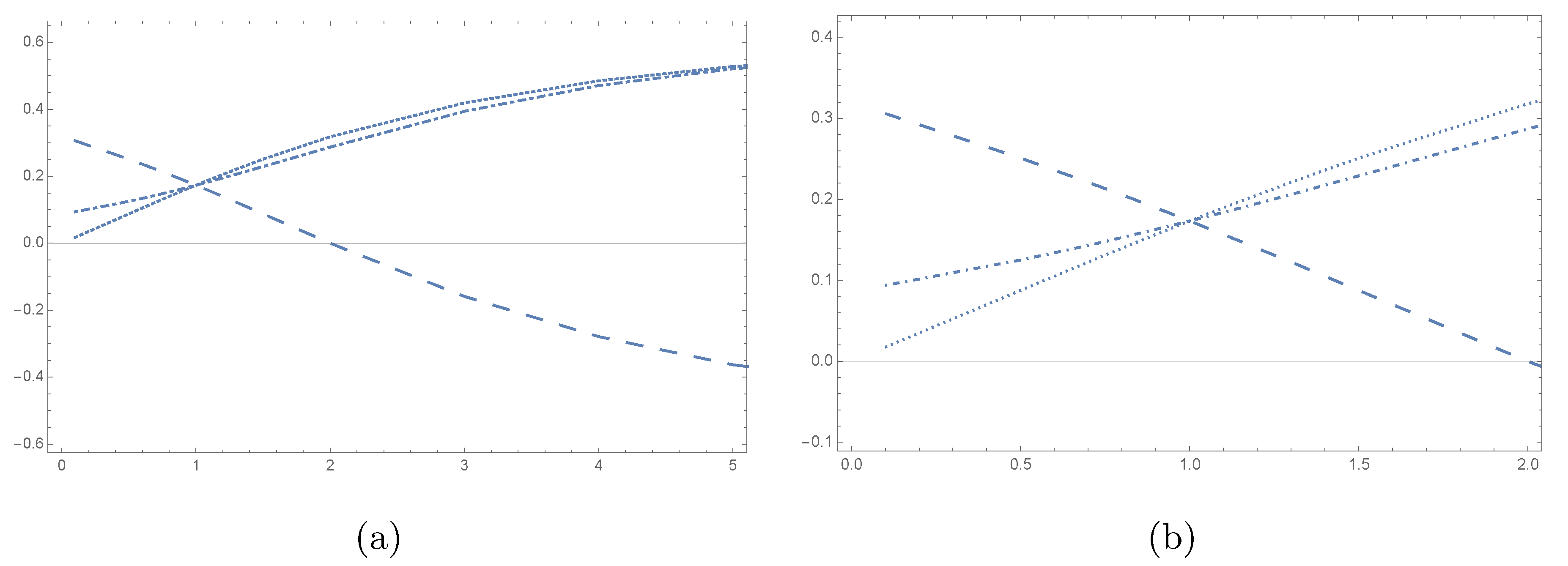
Figure 1. (a) Plot of ${\sigma }_3\left(\alpha \right)$ (dotted), ${\sigma }_2\left(\alpha \right)$ (dashed) and ${\sigma }_1\left(\alpha \right)$ (dot-dashed) as a function of $\alpha \in [0,5]$ for $p=1/4$, $q=1/2$ (b) the same as in (a), for $\alpha \in [0,2]$

Figure 1. (a) Plot of ${\sigma }_3\left(\alpha \right)$ (dotted), ${\sigma }_2\left(\alpha \right)$ (dashed) and ${\sigma }_1\left(\alpha \right)$ (dot-dashed) as a function of $\alpha \in [0,5]$ for $p=1/4$, $q=1/2$ (b) the same as in (a), for $\alpha \in [0,2]$

6. Conclusions

In stochastic thermodynamics the irreversibility of system evolution is expressed in terms of the information $I\left(p\right(\omega \left)\right)$ associated to a trajectory $\omega$ and its time-reversal. The additivity postulate on information $I\left(p\right)$ associated to an event of probability p restricts the possible forms of the average information of the events of information $I\left(p\right)$ to the linear or exponential Kolmogorov-Nagumo mean [11]. In the first case we obtain Shannon information measure and in the second one Rény information measure of order $\alpha$. Note that Rény information measure reduces to Shannon one when $\alpha$ tends to 1.

In stochastic thermodynamics, the entropy production is defined as the linearaverage over the system trajectories $\omega$ of the information difference $I\left(p\left({\omega }_R\right)\right)-I\left(p\left(\omega \right)\right)$ where ${\omega }_R$ is the time-reversed trajectory. This coincides with the linear average of $S\left(\omega \right)=ln[p\left(\omega \right)/p\left({\omega }_R\right)]$ which coincides with the relative entropy $D(p,p_R)$ [2].

In this paper we have shown that, if one considers the exponential average of order $\alpha$ of the above introduced random variables, one obtains three different definitions of the entropy production when one considers trajectories of infinite length which we have called Rény entropy production. It is also shown that in the limit $\alpha$ going to 1 all three definitions reduce to the linear entropy production $\sigma$ in (19) and this result is independent of the order in which the $\alpha$ and n limits are taken. However, Rény information measure is used with $\alpha \ne 1$ in the description of diverse physical systems (turbulent fluid flows, fractal system, DNA sequences, [11]). It is therefore important to investigate the existence of a notion of entropy production associated to Rény entropy via the exponential average. In this respect we have shown that different straightforward generalization of the usual linear average definition are possible, which give quantitatively different answers to the entropy production rate for $\alpha \ne 1$. This fact is relevant for example is one intends to adopt the maximum entropy production rate principle to describe a thermodynamic system in a stationary non equilibrium state ([15,16]). We think that Rény information measure, containing an additional parameter $\alpha$ is able to ’resolve’ the theoretical differences between multiple definitions of the notion of entropy production which remains unseen when considering only the $\alpha =1$ case, corresponding to the use of Shannon entropy. We hope that the issue raised in this work may help to shed light also on the usual notion of entropy production rate, which is a cornerstone of non equilibrium thermodynamics.

References

- De Groot SR, Mazur P.Non-equilibrium thermodynamics. Dover Publications.
- Gaspard P. Time-reversed dynamical entropy and irreversibility in Markovian random processes. Journal of statistical physics. 2004 Nov;117:599-615. [CrossRef]
- Schnakenberg J. Network theory of microscopic and macroscopic behavior of master equation systems. Reviews of Modern physics. 1976 Oct 1;48(4):571. [CrossRef]
- Jiang DQ, Jiang D. Mathematical theory of nonequilibrium steady states: on the frontier of probability and dynamical systems. Springer Science & Business Media; 2004.
- Ge H, Qian H. Physical origins of entropy production, free energy dissipation, and their mathematical representations. Physical Review E—Statistical, Nonlinear, and Soft Matter Physics. 2010 May;81(5):051133. [CrossRef]
- Esposito M, Van den Broeck C. Three faces of the second law. I. Master equation formulation. Physical Review E—Statistical, Nonlinear, and Soft Matter Physics. 2010 Jul;82(1):011143. [CrossRef]
- Busiello, Daniel M., Deepak Gupta, and Amos Maritan. "Entropy production in systems with unidirectional transitions." Physical Review Research 2.2 (2020): 023011. [CrossRef]
- Koralov, Leonid, and Yakov G. Sinai. Theory of probability and random processes. Springer Science & Business Media, 2007.
- Golshani L, Pasha E, Yari G. Some properties of Rényi entropy and Rényi entropy rate. Information Sciences. 2009 Jun 27;179(14):2426-33.
- Rényi A. On measures of entropy and information. In Proceedings of the fourth Berkeley symposium on mathematical statistics and probability, volume 1: contributions to the theory of statistics 1961 Jan 1 (Vol. 4, pp. 547-562). University of California Press.
- Jizba P, Arimitsu T. The world according to Rényi: thermodynamics of multifractal systems. Annals of Physics. 2004 Jul 1;312(1):17-59. [CrossRef]
- Yang YJ, Qian H. Unified formalism for entropy production and fluctuation relations. Physical Review E. 2020 Feb;101(2):022129. [CrossRef]
- Rached Z, Alajaji F, Campbell LL. Rényi’s divergence and entropy rates for finite alphabet Markov sources. IEEE Transactions on Information theory. 2001 May;47(4):1553-61. [CrossRef]
- Masi M. A step beyond Tsallis and Rényi entropies. Physics Letters A. 2005 May 2;338(3-5):217-24. [CrossRef]
- Favretti M. The maximum entropy rate description of a thermodynamic system in a stationary non-equilibrium state. Entropy. 2009 Oct 29;11(4):675-87. [CrossRef]
- Monthus C. Non-equilibrium steady states: maximization of the Shannon entropy associated with the distribution of dynamical trajectories in the presence of constraints. Journal of Statistical Mechanics: Theory and Experiment. 2011 Mar 4;2011(03):P03008. [CrossRef]
- Cybulski, O., Babin, V. and Holyst, R., 2005. Minimization of the Renyi entropy production in the space-partitioning process. Physical Review E—Statistical, Nonlinear, and Soft Matter Physics, 71(4), p.046130. [CrossRef]
Disclaimer/Publisher’s Note: The statements, opinions and data contained in all publications are solely those of the individual author(s) and contributor(s) and not of MDPI and/or the editor(s). MDPI and/or the editor(s) disclaim responsibility for any injury to people or property resulting from any ideas, methods, instructions or products referred to in the content. |
© 2024 by the authors. Licensee MDPI, Basel, Switzerland. This article is an open access article distributed under the terms and conditions of the Creative Commons Attribution (CC BY) license (http://creativecommons.org/licenses/by/4.0/).
Copyright: This open access article is published under a Creative Commons CC BY 4.0 license, which permit the free download, distribution, and reuse, provided that the author and preprint are cited in any reuse.