Submitted:
04 September 2024
Posted:
05 September 2024
Read the latest preprint version here
Abstract
In a V2V communication environment, the control of electric vehicle platoons faces issues such as random communication delays, packet loss, and external disturbances. To address these issues, a robust UKF-MPC-based longitudinal control algorithm for the platoon is designed. First, a longitudinal kinematic model of the vehicle platoon is constructed, and discrete state-space equations are established. The robust UKF algorithm is derived by enhancing the UKF algorithm with Huber-M estimation. This enhanced algorithm is then used to estimate the state information of the leading vehicle. Based on the vehicle state information obtained from the robust UKF estimation, feedback correction compensation is added to the MPC algorithm to design the robust UKF-MPC longitudinal controller. Finally, The effectiveness of the proposed controller is verified through CarSim/Simulink joint simulation. Simulation results show that the robust UKF-MPC longitudinal controller performs better compared to the MPC and UKF-MPC longitudinal controllers. When facing the communication delay and packet loss problems, the robust UKF-MPC longitudinal controller has higher control accuracy and less performance degradation. It has strong robustness and stability.
Keywords:
Electric Vehicle
; Platoon Longitudinal Control
; Model Predictive Control
; Unscented Kalman Filter
1. Introduction
With the popularization of electric vehicles (EVs) and the rapid development of telematics, the intelligent control of EV platoons has become an important application in intelligent transportation systems. This technology can effectively improve transportation safety, enhance efficiency, and reduce energy consumption [1,2].
In EV platoons, vehicles exchange real-time information through wireless communication technologies such as vehicle-to-vehicle (V2V) communication, enabling collaborative control and maintaining desired spacing for safe travel. However, the complexity of traffic environments and the nonlinear nature of vehicle dynamics systems present challenges, including communication delays, data packet loss, and external interference, which can adversely affect vehicle behavior and weaken platoon stability [3,4].
To address these challenges and enhance the stability and control precision of vehicle platoons, numerous researchers have conducted studies. Yang et al. [5] addressed the robustness of cooperative adaptive cruise control (CACC) systems under cyber-attacks by proposing a method to utilize multiple V2V communication networks for data fusion and redundant transmission, and designing an H∞ controller to minimize the impact of sensor and channel noise on vehicle platoon performance. Li et al. [6] proposed a distributed nonlinear vehicle platoon longitudinal controller based on a third-order model for heterogeneous vehicle platoons in communication delay environments. Samii et al. [7] developed a linear predictive feedback Cooperative Adaptive Cruise Control (CACC) controller to address communication and actuator delays in heterogeneous platoons. Halder et al. [8] introduced a discrete-time distributed state feedback control strategy for homogeneous vehicle platoons with an undirected network topology, capable of resisting external disturbances and random continuous network packet losses. Lu et al. [9] created a distributed model predictive control (DMPC) strategy to ensure platoon stability for nonlinear vehicle platoons with a unidirectional communication topology, considering sensor jitter, control delays, and errors in real vehicle conditions. Meng et al. [10] designed a robust MPC controller and a slip ratio controller to address control errors due to parameter uncertainties in platoon modeling and ensure the stability of following vehicles. Tian et al. [11] employed Model Predictive Control (MPC) and Long Short-Term Memory (LSTM) prediction methods to study communication delay compensation in vehicle coordination control under CACC systems. Wang et al. [12] proposed an improved MPC algorithm based on the Kalman Filter (KF) to tackle issues such as environmental disturbances, sensor noise, and poor stability in following time-varying speeds.
In summary, while research on the longitudinal control of EV platoons has progressed in addressing external interference, communication delay, and data packet loss, the randomness of these factors still impacts vehicle state accuracy and platoon stability. To solve these issues, this paper constructs a longitudinal kinematic model of a vehicle platoon and establishes discrete state-space equations. By introducing Huber-M estimation to enhance the UKF algorithm, vehicle state information within the platoon is accurately estimated. Based on this estimated state information, feedback correction compensation is integrated into the MPC algorithm to design a robust UKF-MPC longitudinal controller. Finally, the effectiveness of this controller is verified through CarSim/Simulink co-simulation.
2. Problem Description
Consider a traffic scenario in which N electric vehicles form a platoon travelling in a straight line, as shown in Figure 1, where the leading vehicle is numbered and the following vehicles behind are numbered . The following vehicle in the platoon adopts the Predecessor Following (PF) communication topology form through the V2V communication technology to obtain the position, velocity, acceleration and other state information of the vehicle in front of it. The distance between the following vehicle and the front vehicle is obtained through on-board sensors (e.g., radar, camera, etc.).
3. Longitudinal Kinematic Model of the Vehicle Platoon
Based on the consideration of various factors such as stability, safety and the complexity of the use of working conditions, for the desired distance between neighboring vehicles, the desired distance is more easily adjusted with the Constant Time Headway (CTH) as the vehicle platoon spacing strategy.
where represents the minimum safe distance, represents the headway, represents the velocity of vehicle i.
According to the position information obtained from V2V communication, the workshop distance of adjacent vehicles is calculated. Considering the communication delay problem and for the driving safety, the calculated workshop distance is combined with the workshop distance obtained from the on-board sensors to obtain the workshop distance of the neighboring vehicles, and the calculation formula is as follows:
where and represent the position information of neighboring vehicles, represents the length of vehicle i, represents the weight parameter, and represents the maximum velocity of vehicle i.
According to the longitudinal kinematics between vehicle i-1 and vehicle i, the inter-vehicle spacing error , and the relative velocity , can be calculated as follows:
Considering that there is a time delay problem in the vehicle actuation system, the relationship between the actual acceleration and the desired acceleration of vehicle i is described by adding a first-order inertial link, which is expressed by the following relation:
where K represents the first-order system gain, which takes the value of 1, and represents the inertial link time constant.
According to the above model and longitudinal kinematics a discrete time domain relational equation can be obtained:
where k represents the current moment of the system, k+1 represents the next moment of the system, and represents the sampling time of the system.
Define as the state variable, as the control variable, and as the disturbance variable. Rewrite Equation (7) into the form of discrete state space equations:
The coefficient matrix is , , .
4. Platoon Longitudinal Controller Design
Design the longitudinal controller of vehicle i as an upper and lower layer. The upper controller obtains the state information of the vehicle i-1 and the state information of the vehicle i through the V2V communication to decide the desired acceleration, The lower controller controls the acceleration and deceleration of the vehicle i according to the desired acceleration. Considering that the V2V communication has the problems of random communication delay and data loss, the robust UKF algorithm is used to estimate the state information of the vehicle under the influence of the communication problem. The specific control framework is shown in Figure 2.
4.1. Robust UKF State Prediction Algorithm
Vehicle nonlinear systems:
where represents the state vector, represents the observation vector, represents the state transfer equation, represents the observation equation, represents the system process noise, and represents the observation noise.
The specific steps of robust UKF are as follows:
- 1.
- Initialize the mean and covariance of the initial state of the system .
- 2.
- Calculate the sigma points and construct 2n+1 sigma points along with the corresponding weights.
The weighting coefficients for the mean and covariance are, respectively:
where represents the mean weight factor, represents the covariance weight factor, and represents a non-negative weighting factor to limit the error caused by the higher order terms, taking the value of 2.
- 3.
- Forecast update.
Prediction system sigma point set:
Estimates of the state of the predictive system:
Predicting system state covariance:
where represents the covariance matrix of the system process noise.
- 4.
- Measurement update.
Nonlinear transformation of each Sigma point set using measurement equations.
Estimated value of the measurement:
Measured covariance:
where represents the covariance matrix of the system measurement noise.
- 5.
- Calculate the gain.
Calculation of cross-covariances:
Calculate the Kalman gain:
- 6.
- Huber-M estimation.
Calculate the residuals:
where represents the actual measured value.
Set the threshold parameter:
where , and represent the tuning parameters and represents the diagonal element of the state estimation covariance matrix.
Calculate Huber weights for M estimation.
- 7.
- Measurement correction.
Updated estimates:
Update covariates:
The robustness of the UKF is enhanced by introducing Huber-M estimation to deal with outliers in the observed data.
4.2. Robust MPC Upper Layer Controller
The state space equations for longitudinal kinematics have been obtained above. The workshop distance, workshop distance error, relative velocity between vehicle i-1 and vehicle i, and the velocity and acceleration of vehicle i are chosen as the outputs of the state equations of the system:
Thus, the system state output equation is obtained:
Its coefficient matrix is , .
Introduce control quantities into the state equation to construct new state quantities:
Derive the new state space equation as:
where , , , is the increment of the control quantity, is the dimension of the state quantity, and is the dimension of the control quantity.
The new system state output equation is derived as:
where , represents the dimension of the output quantity.
4.2.1. Feedback Correction Compensation
Vehicles in the process of modeling, due to the interference of the external environment and the influence of the vehicle parameter error and other reasons, the established model has a certain mismatch, so the introduction of feedback correction mechanism to compensate for the prediction error of the following model, improve the model’s prediction accuracy of the state of the following system, and improve the robustness of the controller.
Define the state-volume error between the state-volume and the state-prediction at moment k:
where represents the actual state of vehicle i at moment k, and is the state prediction of the system for moment k at moment k-1.
At moment k-1, the system predicts the amount of state at the moment:
The state prediction is corrected at moment k by the state quantity error:
where represents the correction matrix, and the value range of each element in F is (0, 1).
4.2.2. Predictive Model Derivation
Assuming that the prediction time domain of the system is and the control time domain is , and that the prediction time domain and the control time domain satisfy . Due to the introduction of the feedback correction mechanism, based on the discrete longitudinal motion state space Equation (33), a new model prediction equation of state can be obtained:
where , represent the output quantity matrix and disturbance quantity matrix of the system in the prediction time domain, and represents the control quantity matrix of the system in the control time domain, as shown below:
, , .
, , , is the prediction matrix and is the control matrix as shown below:
, , , , .
4.2.3. Objective Function
The exponential decay function is introduced as the target function reference trajectory to ensure that the reference trajectory changes more smoothly close to the target value, and the target reference trajectory is:
Where , represents the coefficient matrix of the reference trajectory, and the value range of each element is (0,1).
The prediction matrix for the target reference trajectory is:
The objective function is designed in terms of followability and comfort requirements:
Where , Q represents the weight matrix of the output quantity, R represents the weight matrix of the control quantity increment.
4.2.4. System State Constraints
In order to satisfy the requirements of traveling safety, following, and ride comfort of the platoon longitudinal traveling system, the MPC algorithm is constrained to be able to satisfy multiple constraints at the same time by imposing constraints on the output, control, and incremental control quantities of the MPC algorithm.
The constraints to be satisfied during the control of the MPC algorithm are as follows:
where the parameters with min and max in the subscripts are the upper and lower bounds of the system constraints, respectively.
Into matrix form:
where , .
For solving the problem of no solution in the rolling optimization process of MPC algorithm, the hard constraints are relaxed by introducing relaxation factors and relaxation coefficients to extend the feasible domain of the solution, as shown below:
where represents the relaxation factor matrix, , , , , , is the relaxation coefficient matrix as shown below:
4.2.5. Optimization Problem Solving
To avoid the problem of constraint failure due to relaxation factors, a quadratic penalty term for the relaxation factors is introduced into the optimization objective function to limit the range of constraints due to relaxation, then the performance cost function is:
Where , represents the matrix of penalty coefficients for the relaxation factors.
Expanding and ignoring terms not related to , the collation yields:
where , , , .
Transform the performance cost function treatment into a quadratic programming online solution problem with constraints in the form shown below:
where , , .
Substituting the model predicted state equation and the control quantity into the system state constraint (40) yields:
where , , , , , represent the prediction matrix of the relaxation coefficient matrix, and , , , , , represent the prediction matrix of the upper and lower bounds of the output, control, and control increments, respectively.
The upper controller decides the desired acceleration by means of a robust MPC control algorithm.
4.3. Lower Level Controller
4.3.1. Inverse Dynamics Model
According to the vehicle longitudinal kinematics model, the vehicle longitudinal acceleration and deceleration equations of motion are obtained.
Acceleration equations:
where represents the vehicle mass of vehicle i, represents the vehicle rotating mass conversion factor, represents the driving force, represents the air resistance, represents the rolling resistance and represents the ramp resistance.
Deceleration equations:
where represents the desired braking force.
In drive mode, the desired torque of the drive motor is derived from Equation (44):
where represents the acceleration of gravity, represents the rolling resistance coefficient, represents the ramp angle, is the air resistance coefficient, represents the windward area, represents the rolling radius of the wheels, represents the main gear transmission ratio, represents the transmission efficiency of the power transmission system.
In braking mode, the desired brake master cylinder pressure is derived from Equation (45):
where represents the coefficient of proportionality between braking force and brake master cylinder pressure.
4.3.2. PID Lower Controller
As shown in Figure 2, the lower controller part adopts the PID control algorithm, utilizes the form of feed-forward plus feedback, and controls the driving torque and braking pressure based on the inverse longitudinal dynamics model of the vehicle by means of the drive-brake switching strategy, which tracks the desired acceleration obtained from the upper controller.
5. Simulation Analysis
For validating the designed robust UKF-MPC longitudinal controller, a joint simulation platform based on CarSim/Simulink is built to simulate and analyze the longitudinal control of vehicle platoon.
The simulation scenario with no communication delay and no data loss and the simulation scenario with a random communication delay of 10~100 ms and a communication data loss rate of 50% are set up in Simulink, and the fleet of vehicles containing one leading vehicle and three following vehicles is set up in CarSim, with the initial speed of the four vehicles being 0 m/s and the initial inter-vehicle spacing of 3 m. The main parameters of the vehicles used are shown in Table 1.
Set the target speed of the leading vehicle, including acceleration, uniform speed, deceleration of three kinds of driving conditions, the specific parameters are set as shown in Table 2.
The robust UKF-MPC longitudinal controller of this paper is compared and analyzed with the MPC longitudinal controller and the improved UKF-MPC longitudinal controller based on UKF in the scenarios with and without communication delay and data packet loss problems, and the simulation results are shown in Figure 3, Figure 4, Figure 5, Figure 6, Figure 7 and Figure 8.
Under the condition of no communication delay and packet loss, as shown in Figure 3 and Figure 4, the speed and acceleration under the three controllers can stably follow the speed and acceleration of the front vehicle to ensure the stability of the longitudinal motion of the vehicle platoon; however, when comparing the inter-vehicle spacing errors of the vehicles controlled by the three controllers, the inter-vehicle spacing error under the MPC longitudinal controller is about 0.1 m, that under the UKF-MPC longitudinal controller is about is 0.3 m, and the workshop distance error under the robust UKF-MPC longitudinal controller is about 0.04 m, as shown in Figure 5. It can be seen that the robust UKF-MPC longitudinal controller in this paper improves the control accuracy of the longitudinal motion of the vehicle platoon compared to the MPC longitudinal controller and the UKF-MPC longitudinal controller under the condition of no communication delay and packet loss.
Under the condition of communication delay and packet loss, as shown in Figure 6, the speeds under the three controllers can basically follow the speed of the front vehicle, but the speed of the vehicle controlled by the MPC longitudinal controller jerks at higher speeds; as shown in Figure 7, the acceleration under the MPC controller oscillates violently, the acceleration under the UKF-MPC longitudinal controller jerks slightly and the acceleration under the robust UKF-MPC longitudinal controller jerks less and is basically stable. As shown in Figure 8, the workshop distance error under the MPC longitudinal controller is about 3 m, and the oscillation is violent, the workshop distance error under the UKF-MPC longitudinal controller is about 0.35 m, and there is a jitter when the speed is higher, and the workshop distance error under the robust UKF-MPC longitudinal controller is about 0.045 m, and it is basically stable. It can be seen that the MPC control algorithm is not effective under the condition of having communication random delay and packet loss, while the UKF-MPC control algorithm and the robust UKF-MPC control algorithm can effectively solve the problem of communication delay and packet loss, but the robust UKF-MPC control algorithm is more stable and has higher accuracy.
6. Conclusions
In this paper, a robust UKF-MPC based longitudinal controller for electric vehicle platoon is designed and validated by simulation comparison with MPC longitudinal controller and UKF-MPC longitudinal controller for continuous acceleration and deceleration conditions with and without communication problems.
The simulation results show that under the conditions of no communication delay and packet loss, the proposed robust UKF-MPC controller reduces the vehicle spacing error compared with the MPC and UKF-MPC longitudinal controllers, and improves the control accuracy. Under the conditions with communication delay and packet loss, the MPC longitudinal controller’s performance significantly degrades, which seriously affects the traveling safety and ride comfort. However, the robust UKF-MPC longitudinal controller still maintains a small inter-vehicle distance error and good stability.
Author Contributions
Conceptualization, Z.Lin and H.F.; methodology, Z.Lin; software, Z.Lin and Z.Luo; validation, Z.Lin and Z.Luo; formal analysis, Z.Lin; investigation, X.Z.; resources, J.B. and H.J.; data curation, Z.Lin and H.F.; writing—original draft preparation, Z.Lin; writing—review and editing, Z.Lin, J.B. and H.J.; visualization, Z.Lin; supervision, J.B. and H.J.; project administration, J.B. and H.J.; funding acquisition, H.J. All authors have read and agreed to the published version of the manuscript.
Funding
This research was funded by National Natural Science Foundation of China (52262052) and Innovation-driven Major Project of Guangxi Province (AA22372, AA23062003).
Institutional Review Board Statement
Not applicable.
Informed Consent Statement
Not applicable.
Data Availability Statement
Data are contained within the article.
Conflicts of Interest
The authors declare no conflict of interest.
References
- Indu, K.; Aswatha Kumar, M. Electric vehicle control and driving safety systems: A review. IETE Journal of Research 2023, 69, 482–498. [Google Scholar] [CrossRef]
- Caruntu, C.F.; Braescu, C.; Maxim, A.; Rafaila, R.C.; Tiganasu, A. Distributed model predictive control for vehicle platooning: A brief survey. ICSTCC 2016, 644–650. [Google Scholar]
- Shen, Z.; Liu, Y.; Li, Z.; Wu, Y. Distributed vehicular platoon control considering communication delays and packet dropouts. Journal of the Franklin Institute 2024, 361, 106703. [Google Scholar] [CrossRef]
- Zhao, C.; Cai, L.; Cheng, P. Stability analysis of vehicle platooning with limited communication range and random packet losses. Internet of Things Journal 2020, 8, 262–277. [Google Scholar] [CrossRef]
- Yang, T.; Murguia, C.; Nešić, D.; Lv, C. A Robust CACC Scheme Against Cyberattacks Via Multiple Vehicle-to-Vehicle Networks. IEEE Transactions on Vehicular Technology 2023, 72, 11184–11195. [Google Scholar] [CrossRef]
- Li, Y.; He, C.; Zhu, H.; Zheng, T. Nonlinear longitudinal control for heterogeneous connected vehicle platoon in the presence of communication delays. Acta Automatica Sinica 2021, 47, 2841–2856. [Google Scholar]
- Samii, A.; Bekiaris-Liberis, N. Robustness of string stability of linear predictor-feedback CACC to communication delay. ITSC 2023, 4853–4858. [Google Scholar]
- Halder, K.; Gillam, L.; Dixit, S.; Mouzakitis, A.; Fallah, S. Stability Analysis With LMI Based Distributed H∞ Controller for Vehicle Platooning Under Random Multiple Packet Drops. IEEE Transactions on Intelligent Transportation Systems 2022, 23, 23517–23532. [Google Scholar] [CrossRef]
- Lu, R.; Hu, J.; Chen, R. Cooperative adaptive cruise control of intelligent vehicles based on DMPC. Autom Eng. 2021, 43, 1177–1186. [Google Scholar]
- Meng, J.; Li, C.; Jing, H.; Tong, Y.; Feng, H. Longitudinal Platoon Control of Electric Vehicle Based on Model Predictive Control. Journal of Dynamics and Control 2023, 21, 44–53. [Google Scholar]
- Tian, B.; Yao, K.; Wang, Z.; Gu, G.; Xu, Z.; Zhao, X.; Jing, J. Communication delay compensation method of CACC platooning system based on model predictive control. Journal of Traffic and Transportation Engineering 2022, 22, 361–381. [Google Scholar]
- Wang, Q.; Jiang, J.; Lu, Z.; Zhang, H. Research on cooperative adaptive cruise control strategy based on improved MPC. Journal of System Simulation 2022, 34, 2087–2097. [Google Scholar]
Figure 1.
Schematic diagram of the longitudinal movement of the vehicle platoon.
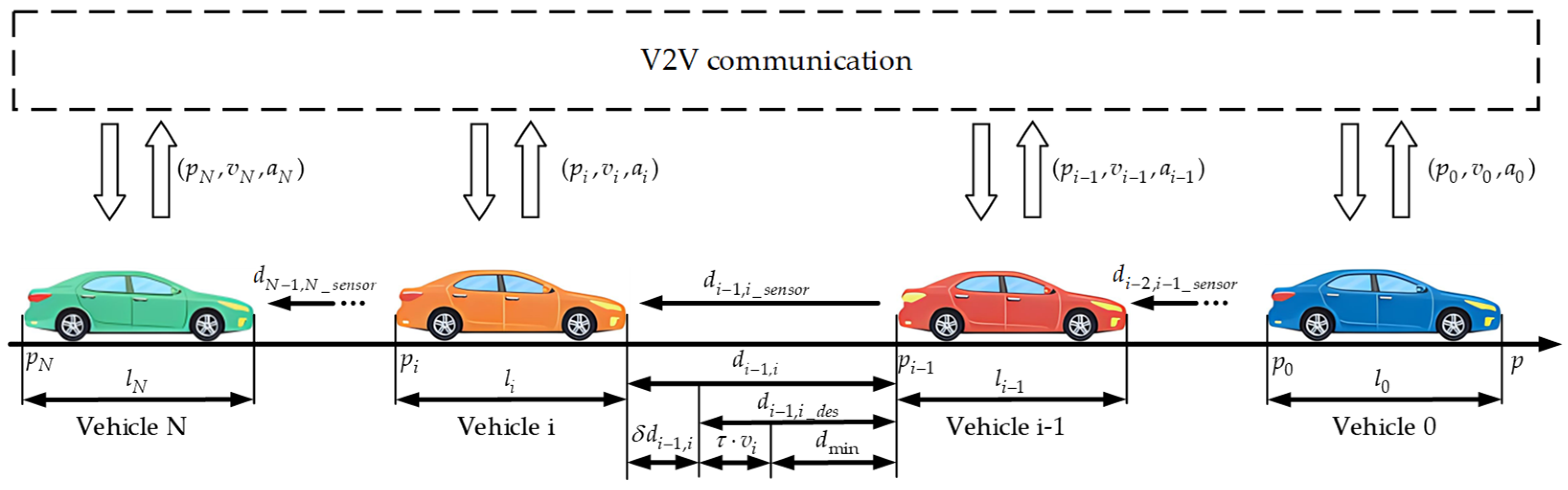
Figure 2.
Framework diagram of robust UKF-MPC based longitudinal controller.
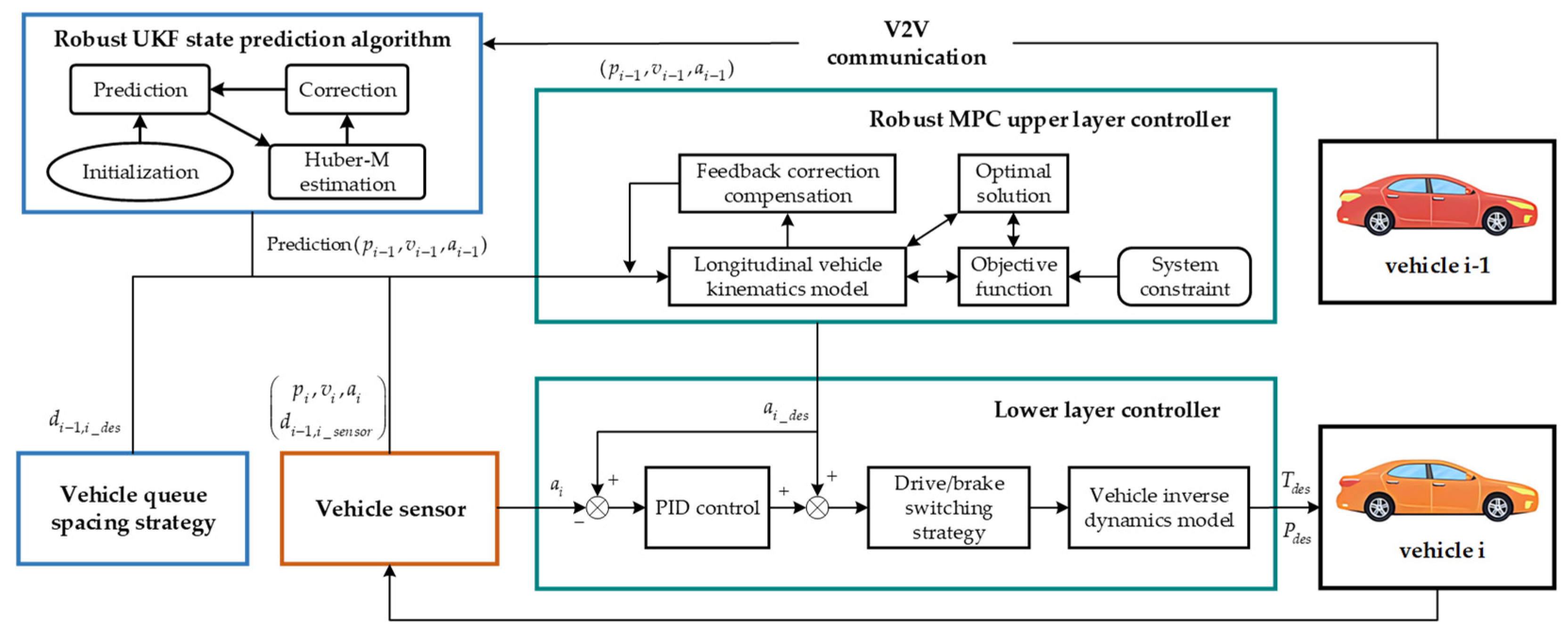
Figure 3.
Variation of velocity under different controllers in an environment without communication delay and data loss.
Figure 3.
Variation of velocity under different controllers in an environment without communication delay and data loss.
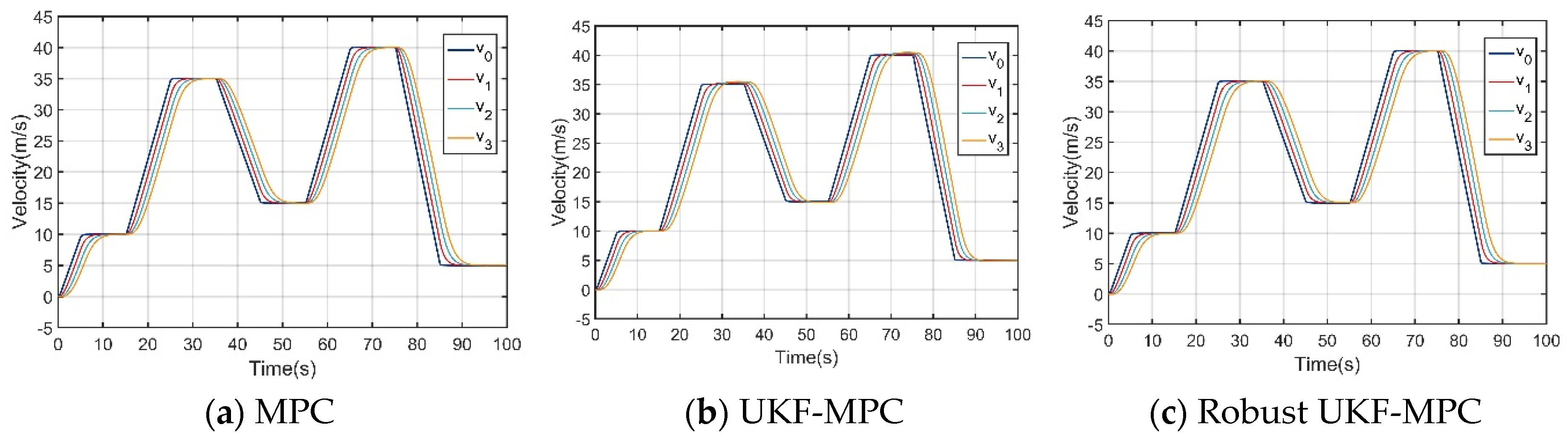
Figure 4.
Variation of acceleration under different controllers in an environment without communication delay and data loss.
Figure 4.
Variation of acceleration under different controllers in an environment without communication delay and data loss.
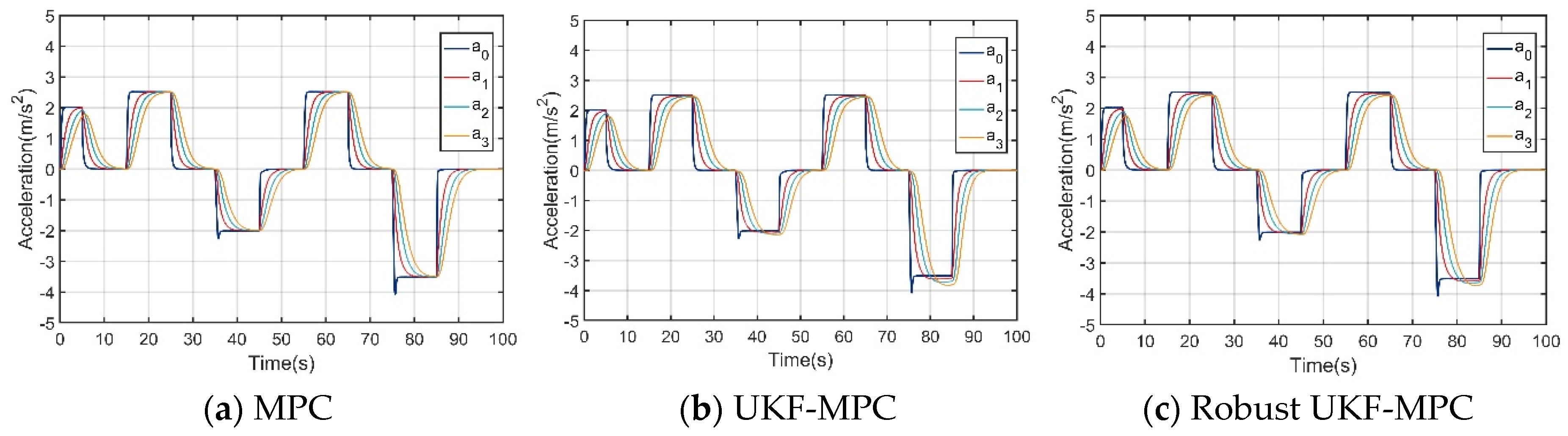
Figure 5.
Variation of spacing error under different controllers in an environment without communication delay and data loss.
Figure 5.
Variation of spacing error under different controllers in an environment without communication delay and data loss.
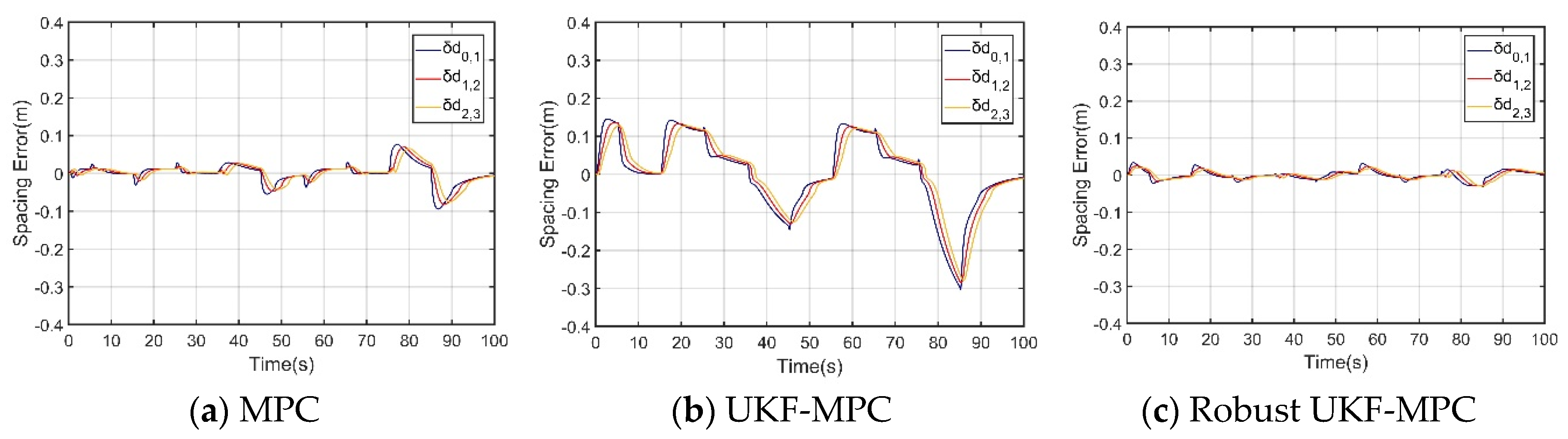
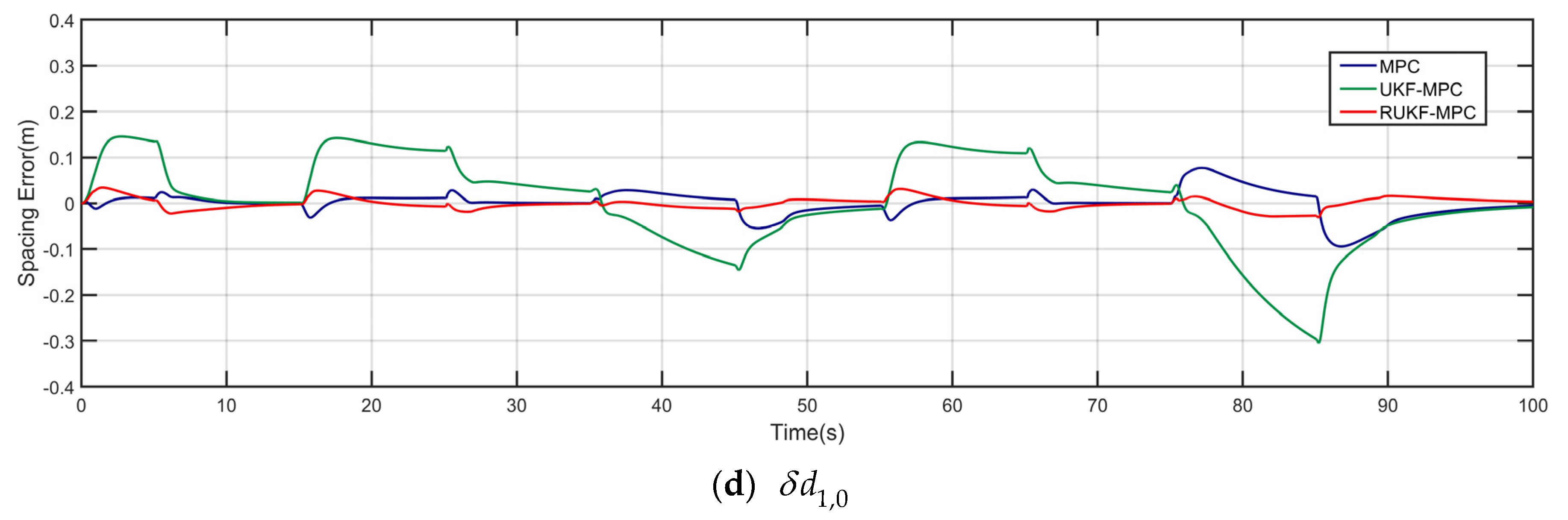
Figure 6.
Variation of velocity under different controllers in an environment with communication delay and data loss.
Figure 6.
Variation of velocity under different controllers in an environment with communication delay and data loss.
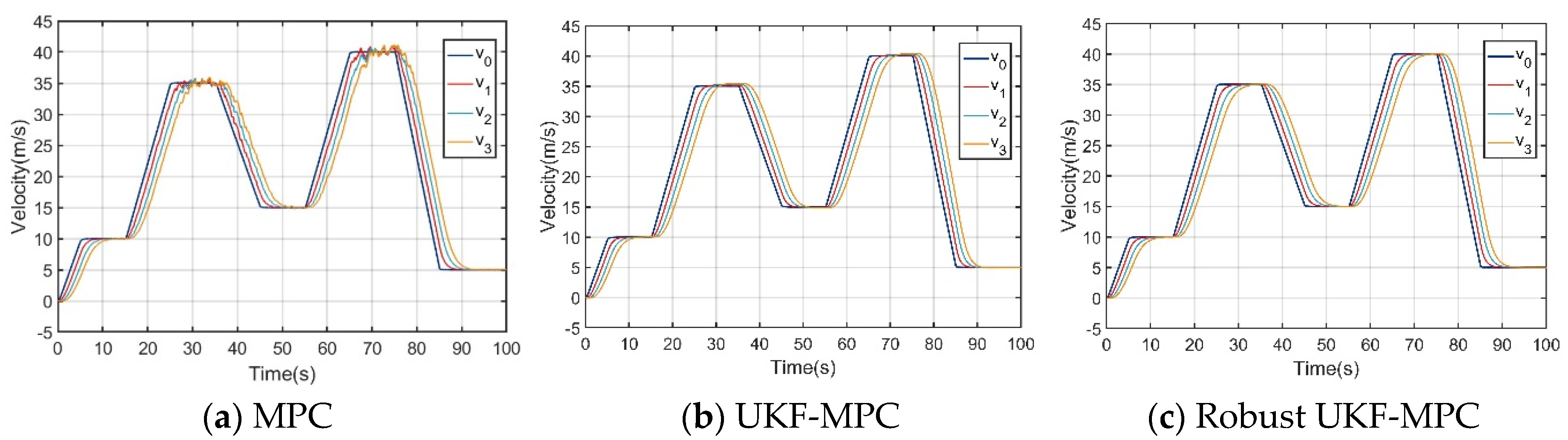
Figure 7.
Variation of acceleration under different controllers in an environment with communication delay and data loss.
Figure 7.
Variation of acceleration under different controllers in an environment with communication delay and data loss.
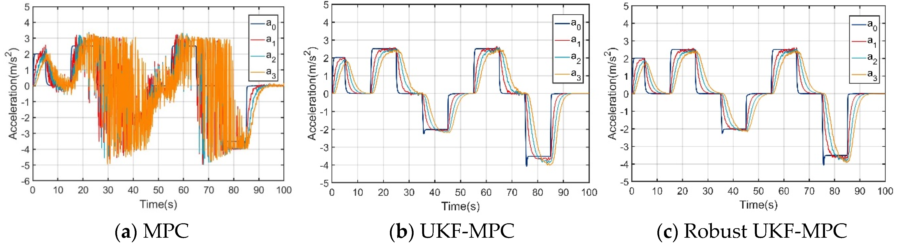
Figure 8.
Variation of spacing error under different controllers in an environment with communication delay and data loss.
Figure 8.
Variation of spacing error under different controllers in an environment with communication delay and data loss.
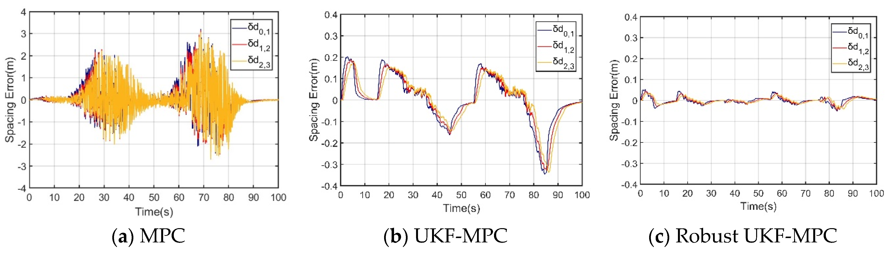
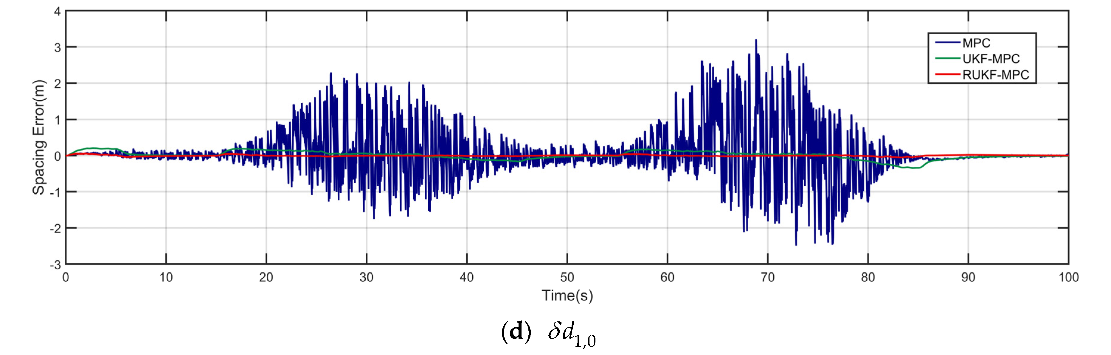

Table 1.
Main vehicle parameters.
| Vehicle parameters | numerical value |
|---|---|
| Vehicle quality, | 1270 kg |
| Vehicle length, | 4 m |
| Wheel rolling radius, | 0.325 m |
| Vehicle windward surface area, | 2.3 m2 |
| Atmospheric drag coefficient, | 0.342 |
| Transmission efficiency, | 0.9 |
| Rolling resistance coefficient, | 0.02 |
Table 2.
Target speeds for leading vehicles.
| Simulation time () | Target velocity ( ) |
|---|---|
| 0≤t≤5 | 2t |
| 5<t≤15 | 10 |
| 15<t≤25 | 10+2.5(t-15) |
| 25<t≤35 | 35 |
| 35<t≤45 | 35-2(t-35) |
| 45<t≤55 | 15 |
| 55<t≤65 | 15+2.5(t-55) |
| 65<t≤75 | 40 |
| 75<t≤85 | 40-3.5(t-75) |
| 85<t≤100 | 5 |
Disclaimer/Publisher’s Note: The statements, opinions and data contained in all publications are solely those of the individual author(s) and contributor(s) and not of MDPI and/or the editor(s). MDPI and/or the editor(s) disclaim responsibility for any injury to people or property resulting from any ideas, methods, instructions or products referred to in the content. |
© 2024 by the authors. Licensee MDPI, Basel, Switzerland. This article is an open access article distributed under the terms and conditions of the Creative Commons Attribution (CC BY) license (http://creativecommons.org/licenses/by/4.0/).
Copyright: This open access article is published under a Creative Commons CC BY 4.0 license, which permit the free download, distribution, and reuse, provided that the author and preprint are cited in any reuse.


