
Submitted:
24 November 2023
Posted:
24 November 2023
You are already at the latest version
Abstract
Intelligent ship technology is currently an international research hotspot, and model predictive control is widely used in the path-tracking control of intelligent vehicles. To construct an intelligent ship anti-disturbance path-tracking control method, firstly, an environmental disturbance model was constructed with the actual meteorological data of the target sea area. Secondly, the Fossen ship equation of motion is linearized and discretized as the ship motion model. Thirdly, the expression of the prediction equation is derived from the ship motion model. Fourthly, the cost function is constructed by using the polar diameter and polar angle values of the ship. Fifth, the power function in the cost function is replaced with an exponential function to obtain an improved cost function. Sixthly, according to the Lyapunov theory and the MPC terminal constraint theory, the stability of the improved cost function is verified. Seventh, different test paths are set up, the environmental disturbance model is taken as the external disturbance, the ship motion model, the prediction equation, and the improved cost function are used to design the anti-disturbance path-tracking control algorithm according to the model prediction control idea for simulation experiments. Finally, different MATLAB simulation results show that the improved cost function can resist disturbance of the external wave, current, and wind, and effectively track the target path. Therefore, this study provides a reference for improving the navigation safety of ship path-tracking.
Keywords:
Ship path-tracking
; External meteorological disturbance
; Model Predictive Control
; Cost function
; MATLAB simulation
1. Introduction
Intelligent ship technology is widely applied to economic construction or military industry, all the world's maritime powers are actively studying intelligent ship technology, so the study of ship path-tracking problems is of great significance. The target path for a path-tracking problem is fixed, which is different from the trajectory following. There may be differences in the formulation of these two problems in different articles, and we will divide the problems into two categories according to whether the path changes over time. The ship path-tracking problem is a nonlinear control problem, this field has been associated with a lot of research results.
The meaning of trajectory tracking mentioned is the same as path-tracking. [8] described both the trajectory tracking methods and the most commonly used trajectory tracking controllers of autonomous vehicles, besides state-of-the-art research studies of these controllers. [17] they highlighted vessel autonomy, regulatory framework, guidance, navigation and control components, advances in the industry, and previous reviews in the field. In addition, they analyzed the terminology used in the literature and attempt to clarify ambiguities in commonly used terms related to path planning. [1] found the need for a unified platform for evaluating and comparing the performance of algorithms under a large set of possible real-world scenarios. [15] considered autonomous ships are expected to improve the level of safety and efficiency in future maritime navigation. [20] provided a review of recent progress in the context of motion planning and control for Autonomous marine vehicles (AMVs) from the perceptive of model predictive control (MPC).
[16] reviewed the main control schemes, including proportional-integral-derivative (PID)-based, sliding mode control (SMC)-based, adaptive-based, observation-based, model predictive control (MPC)-based combined control techniques, to consolidate the main efforts made by the automatic control community in this field over the last two decades. [12] developed a model predictive controller for a 3 Degrees of Freedom (DOF) unified maneuvering model of the KVLCC2 crude oil tanker. The rudder control was exerted by a nonlinear model predictive controller and the effectiveness of the controller was studied.
[18] employed a nonlinear model predictive control (NMPC) model based on an accurate ship motion model to control the trajectory tracking, efficiently improving the anti-disturbance capability. [21] presented a weight optimization method for a nonlinear MPC (NMPC) based on the genetic algorithm (GA) for ship trajectory tracking. [7] used the model predictive control (MPC) method under constraints to track planned trajectories and optimize motion processes, while ensuring control stability through Lyapunov's theorem. [2] applied a practical nonlinear model predictive control strategy to reduce the computational cost considerably, given the non-negligible computational cost of such a nonlinear predictive guidance strategy.
After learning the research points of above authors, we found that most of the current papers in the field of ship path-tracking only considered the influence of current or wind, and few papers considered the common disturbance of wave, current, and wind together. Therefore, we consider the environmental disturbance and study the application of model predictive control algorithm in the field of ship path-tracking. In particular, we use real meteorological data to construct an environmental disturbance model, use polar diameter and polar angle to construct the path-tracking cost function of underdriven ships, change the fourth-order exponential function to an exponential function, and perform the stability analysis. Finally, Different path-tracking experiment shows that the ship can resist the disturbance of external wave, current, and wind, and track the target path effectively.
Section 1 introduces the significance and status of the path-tracking control problem, as well as the main contents of our research. Section 2 introduces the distribution of wave, current, and wind, and constructs environmental disturbance models. Section 3 introduces the ship's motion model, prediction equations, cost function, improved cost function, and stability analysis. Section 4 introduces the ship anti-disturbance path-tracking control algorithm, and studies the effect of the algorithm in different usage scenarios. Section 5 introduces the conclusions and implications based on the research content of this paper.
2. Environmental disturbance model
Wave, current, and wind loads affect a ship’s movement [4]. To accurately simulate the actual working conditions of the ship, first, the actual wave, current, and wind data of the target sea area were obtained from the major meteorological data platforms, and then, the effective data were used to calculate the change laws of the wave, current, and wind; next, an environment disturbance model were constructed according to the statistical laws, and finally, the environment disturbance model were used as the disturbance item to study the performance of the ship tracking the target path.
2.1. Wave
The actual wave data used in this study were obtained from the National Marine Science Data Center [10]. As shown in Figure 1, from January 1996 to October 2001, the maximum wave height (MH) (m) of the target sea area followed these patterns: The max wave height was concentrated between 0 m and 2.3 m and rarely 2.3 m to 10 m. The distribution of the max wave height was approximately a normal distribution.
2.2. Current
The current dataset from Marine Science Big Data Center [5,9]. As shown in Figure 2, From January 1997 to December 2016, the surface current of 1 square nautical mile in the target sea area had the following characteristics: The maximum combined velocity of the current (MC) (m/s) did not exceed 0.8 m/s, and the distribution of the current combined velocity approximately met the normal distribution.
2.3. Wind
The mixed wind dataset was obtained from the National Environmental Information Center (NCEI) of the National Oceanic and Atmospheric Administration (NOAA) [11]. As shown in Figure 3, From 2002 to 2018, the characteristics of the wind data at 10 m above the target sea area were as follows: The maximum combined velocity of wind (MW) (m/s) was close to 24 m/s, the maximum frequency of combined velocity was about 7.8 m/s, and the statistical histogram of combined velocity frequency distribution approximately met the normal distribution.
2.4. External meteorological model
It is assumed that meteorological conditions remain largely unchanged in the last 30 years. According to the probability density function in Figure 1 , Figure 2, and Figure 3 three groups of arrays MH ~ N (, ), MC ~ N (,), and MW ~ N (, ), be generated that conform to the corresponding normal distribution. After reordering, three groups of arrays (MH0, MC0, MW0) were obtained, this is the environment disturbance model, as shown in Figure 4. The X-axis represents position, and the Y-axis represents the values of wave, current, and wind and the change rate of corresponding values.
The wave, current, and wind values in the figure demonstrate trends from a small value to a medium value, then to a large value, then to a medium value, and finally to a small value. The wave, current, and wind values first increase slowly, then increase rapidly, then decrease rapidly, and finally decrease slowly. The location of the maximum values of wave, current, and wind is the same, and this location produced the maximum disturbance. Therefore, this environment disturbance model was used as the external disturbance of the ship.
3. Model predictive control algorithm
Model predictive control (MPC) is easy to realize multi-objective cooperative control, and has advantages in dealing with multi-input multi-output systems, complex constraint problems, and system nonlinear problems. Therefore, we use the idea of this algorithm to construct a ship anti-disturbance path-tracking method.
Only the 3 DOF of surge, sway, and yaw had to be considered in path-tracking problems. As is shown in Figure 5, the path-tracking problem is to let the ship's position track the target position . The origin of body coordinate frame is fixed at the center of gravity of the ship, points to the front of the ship, points to the right of the ship, and points clockwise. The origin of the global coordinate frame is fixed on the section of the earth's surface, represents to the north direction, represents to the east direction, and denotes the heading angle between the heading and the north direction. There is a load angle between the environment disturbance and the heading of the ship.
3.1. Model of ship motion
The Fossen model [13] Equation (1) in the body coordinate frame is given by:
The parameters corresponding to this expression are as follows:
Using the wave load formula in [19], and using the current load formula [3] which is similar to the wind load formula in [14]. The wave load is represented by Equation (3), the current load is represented according to Equation (4), and the wind load is represented by Equation (5).
The ship motion model Equation (1) - (5) is regarded as a state-space control system with as states, as inputs, and as disturbances. The parameters are explained in the above relevant literature, and we set specific parameter values according to the physical conditions of the actual ship, and the value of is taken from (MH0, MC0, MW0).
The first-order linear equations of the ship's longitudinal, transverse, and yaw directions can be obtained by Taylor Formula. Then, the Euler’s method is used to obtain the discretized ship motion Equation (6). Equation (6) takes the velocities of the ship as the states.
Multiply both sides of the Equation (6) by the sampling period to get Equation (7). Equation (7) uses the positions of the ship as states.
3.2. Prediction expression
Using the discretized first-order ship motion Equation (7), a new state-space expression and output expression are constructed, as shown in Equation (8).
Including:
According to the Equation (8), the position of the ship in the global coordinate frame at the next time is obtained:
After derivation, the prediction expression of the system is expressed as:
3.3. Cost function
It is shown in Equation (11), that we combine the ship position states and in the global polar coordinate system to obtain the global polar diameter position , and obtain the global polar angle position according to the heading position .
In this way, we can accurately track any target path by controlling the polar diameter and polar angle of the ship separately in the global polar coordinate system. Simultaneously, it is necessary to avoid sudden changes in the control quantity at each time. Accordingly, the cost function of the ship's radial motion and the ship's heading motion is given by Equation (12).
The cost function consist of and , is the current moment, is the number of predicted steps, is the number of control steps, are weight matrix. The constraint expression of the ship control quantity and and the constraint expression of the control increment and , is shown in Equation (13). The goal of optimization is to find the optimal amount of control for each step, as shown in the Equation (14).
4. Algorithm improve and analysis
4.1. Artificial potential field
The attractive field formula of the artificial potential field method [6] is shown in Equation (15), where is the scale factor, represents the distance from the current position to the target position , and is the distance domain value. According to the Equation (15), we know that within the distance , the greater the distance from the current position to the target position, the greater the attraction.
From the characteristics of the attractive field formula Equation (15) and the corresponding gradient formula, we know that when the gradients in both directions of the original cost function are equal. It does not distinguish the magnitude of the respective effects of the two variables and .
4.2. Improved cost function
We replace one power function of the original cost function with an exponential function and obtain a new cost function , as show in the below.
The value of the cost function becomes larger as the current variable moves away from the target variable , and smaller as the current variable moves closer to the target variable , so the minimum value of the cost function is always achieved at .
According to the characteristics of the cost function the polar diameter is taken as the greater descending direction and the control quantity is taken as another direction. Then, the improved cost function Equation (17) is obtained.
The improved cost function consist of and , is the current moment, is the number of predicted steps, is the number of control steps, are weight matrix. The constraint expression of the ship control quantity and and the constraint expression of the control increment and , is shown in Equation (18). The goal of optimization is to find the optimal amount of control for each step, as shown in Equation (19).
4.3. Stability Analysis
Lyapunov theorem:
is the time, is a stable equilibrium point of , and is asymptotically stable. Such a function is called Lyapunov function.
Assumed function expression is as follows:
In the above expression, the weight matrix , the prediction step is , and the control step is , represents the polar diameter of the ship at time in the global coordinate system, represents the target polar diameter value at time in the global coordinate system, represents the increment of polar diameter control quantity.
Set terminal constraints for the states of the system.
represents terminal constraint set, represents control law set, represents the polar diameter control law, represents the polar angle control law.
When , polar diameter control increment becomes 0, and the function becomes:
Since the ship control system is stable, there are
Where is the lower limit of , is the upper limit of , in other words is bounded, moreover the system state has terminal constraints. As long as the appropriate control quantity is selected, the system can always make the bounded value converge to zero.
The process of tracking the path is the process of tracking each target path point with the increase of time . The polar direction uses the step prediction tracking method each time, and each solution results in an optimal solution sequence , select the first pole diameter optimal control quantity to obtain the corresponding function and .
In the time of
Let
Here
Therefore
At , after the optimal solution control quantity was inputed into the system
Due to the terminal constraints of system states, such that so
Here is the derivation
And we can get:
To sum up: The function satisfies the stability condition of the Lyapunov function, the zero point is an equilibrium point, and the function is globally asymptotically stable.
5. Path-tracking experiment simulation
5.1. Experimental setup
Different paths were set: 1) Straight line . 2) cycle line . 3) outline of SMU-Smart Lake. External meteorological disturbance model (MH0, MC0, MW0) was introduced. Nonlinear ship motion model Equation (7) was used. The improved cost function and the original cost function were adopted, respectively.
5.2. Path-tracking algorithm
The algorithm of path-tracking is shown below.
| Path-tracking MPC algorithm |
|
1. Design the target path
)
according to the two polar parameters and store the target path in discrete form. 2. Set the sampling period , predict step size , initial control quantity initial state variables 3. Set parameters such as the ship's mass, moment of inertia, damping coefficient, and additional mass. 4. Set parameters such as encounter angle, density, speed, drag coefficient, cross-sectional area, and ship length. 5. According to the environment disturbance model, set their respective sequences 6. Calculate the load of wave, current, and wind, and obtain the longitudinal disturbance load , the lateral disturbance load , and the yaw direction disturbance load Obtain the longitudinal disturbance lateral disturbance , and yaw direction disturbance Update parameters of ship motion equation and parameters of wave, current, and wind. Update the position equation Calculate the heading prediction state matrix predictive control matrix From the above prediction matrix, the prediction heading of the future is From the radial motion equation of the ship is obtained. According to the expression of , the cost function coefficient matrix is determined. Obtain the target pole diameter value from the target path . Let Cost function with constraints Gradient descent algorithm is used to solve the function with as the variable, is obtained. If the amount of control for the first few steps is too small, set the amount of control to a large value to speed up tracking. Take stored in variables Bring into the function to get the position at the next moment. Radial prediction position at the next moment Starting from the polar angle value of the target path, take continuously to obtain Construct the cost function of pole angle The quadratic programming algorithm is used to solve the quadratic function with as the variable to obtain the Take stored in variables Bring into the function to get the heading of the next moment. Subtract the from the , respectively, and divide the difference by to get the new Draw the target path, follow path, control quantity, etc. separately. |
5.3. The impact of disturbance
First, the rudder angle control amount was fixed at 0, the longitudinal control amount was set to 100000, and the influence of external disturbance on the ship's motion is shown in Figure 6. Then the rudder angle control amount was set to 10000, the longitudinal control amount was fixed to 0, and the test results of external disturbances affecting the ship's movement are shown in Figure 7.
As observed from Figure 6 and Figure 7, under the influence of wave, current, and wind the ship's path is shifted, when there was no rudder angle with a constant driving force, the ship's motion track is approximately S-shaped, and when there is no driving force with constant rudder angle, the ship movement is negligible, and the path of movement is approximate to a combined spiral.
5.4. Line and circle path-tracking
The linear path-tracking and the circular path-tracking simulation results are shown in Figure 8 and Figure 9, respectively.
The tracking polar diameter curve is slightly smaller than the target polar diameter curve, and the tracking polar angle curve is stable after catching up with the target polar angle curve. The tracking line coincides with the target line, and the tracking line is slightly larger than the target line. With the increase of control steps, the polar diameter control quantity gradually increases according to a certain slope after catching up with the target polar diameter, and the polar angle control quantity is stable at zero after catching up with the target polar angle. As the external wave, current, and wind changed over time, the tracking path offset of the ship's heading was not affected. Overall, the straight-line path-tracking effect is desirable.
The tracking polar diameter value is slightly less than the target polar diameter value before the maximum of the target polar diameter value, the tracking polar diameter value is slightly greater than the target polar diameter value after the maximum of the target polar diameter value, and the tracking polar angle curve is slightly less than the target polar angle curve after catching up with the target polar angle curve; The diameter of the tracking curve is slightly smaller than that of the target circle, and the circular tracking error increases from small to large and then decreases. With the increase of control steps, the pole diameter control value decreases from a large positive value to zero and then changes to a large negative value, and the pole angle control value decreases from a large negative value to zero and then changes to a small positive value and is stable. From the results of the simulation, the influence of the external wave, current, and wind on the path of the ship has been compensated by the control variable. Overall, circular path-tracking works as desired.
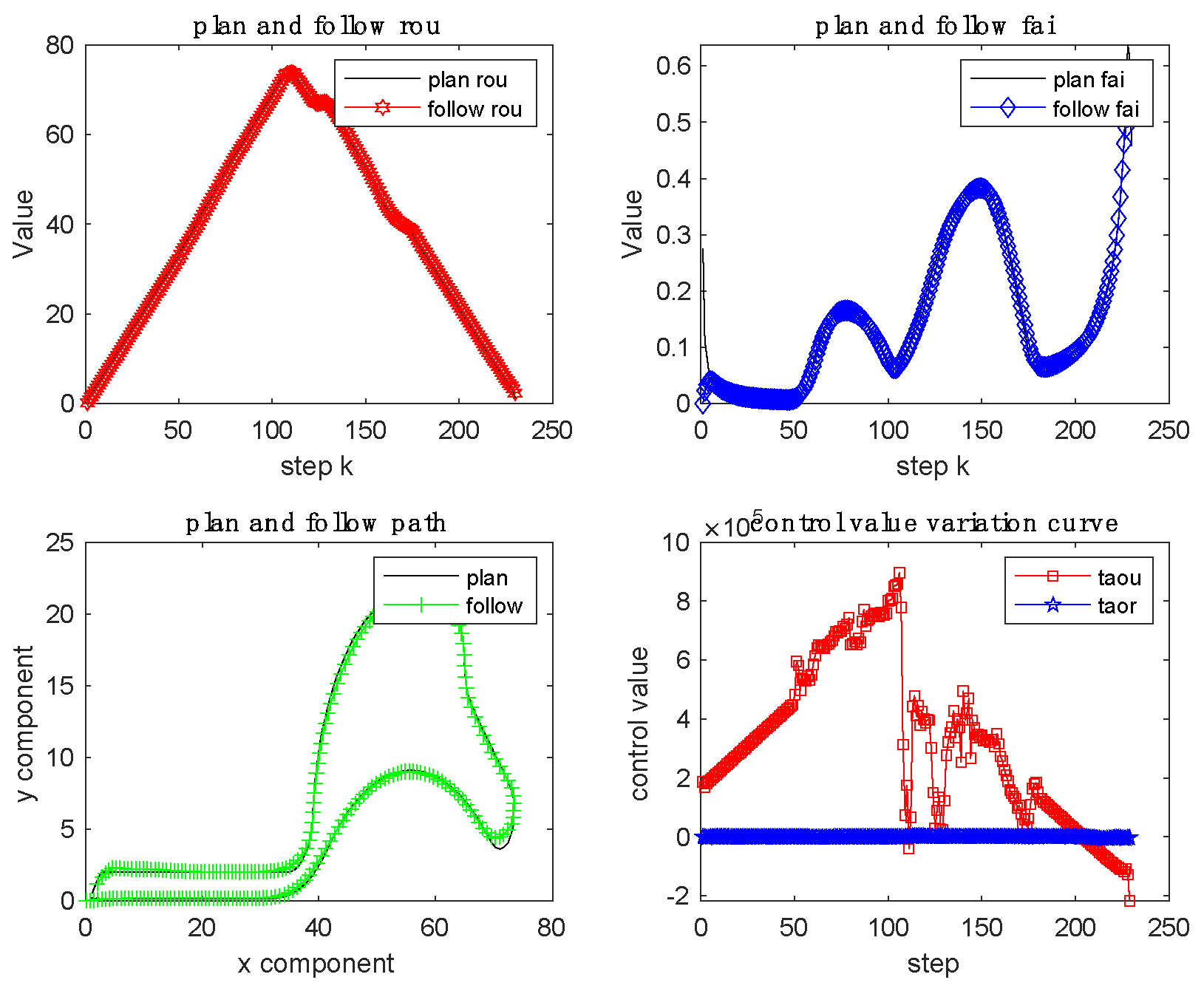
5.5. Complex curve path-tracking
Since the outline of SMU-Smart Lake is composed of curves with different curvatures, we use the contour curve of SMU-Smart Lake to perform the path-tracking test. According to the contour curve of SMU-Smart Lake, the target path is drawn, the environmental disturbances model (MH0, MC0, MW0) were added to the path, and the path-tracking simulation test is performed using the original cost function and the improved cost function, respectively. After simulation, the path-tracking results of the improved cost function and the original cost function are shown in Figure 10 and Figure 11, respectively.
It can be seen from the SMU-Smart Lake tracking path-tracking process in Figure 10 that when the curvature of the target curve changes significantly, the deviation between the tracking curve and the target curve is large, this shows that when the curvature of the target path is large, the tracking effect of the improved cost function is limited. If the external environmental disturbance changes abruptly, the tracking curve will change, and the tracking control amount will also change accordingly. Comparing the simulation results of Figure 11 with Figure 10, we can find that the two are almost the same, so it is believed that the improved cost function can also better realize the function of resisting environmental disturbances and tracking the target path.
6. Summary
This work studies the ship anti-disturbance path-tracking from the following aspects: the status of the problem, the wave, current, and wind disturbance model, the ship motion model, prediction expression, cost function, improved cost function and stability analysis, path-tracking experimental analysis. Further, the simulation results of this paper can enable intelligent ships to achieve control objectives more flexible and maneuverable, and improve ship safety in path-tracking. For more rigorous outcomes, the simulation experiment results herein must be further verified by testing the actual system. For the problem of anti-disturbance path-tracking introduced in this paper, solving it demands a set of mathematical equations and control theories. Nevertheless, these equations and theories are complex, abstract, and time-consuming to understand, which hinders the widespread adoption of this technology. Therefore, it is vital that a simpler and more accessible approach be developed in the future. Moreover, Intelligent vehicle companies and research institutes are paying close attention to this technology, which once matures will help promote the development of Intelligent ships.
References
- Vagale, A.; Bye, R.T.; Oucheikh, R.; Osen, O.L.; Fossen, T.I. Path planning and collision avoidance for autonomous surface vehicles II: a comparative study of algorithms. J Mar Sci Technol 2021, 26, 1307–1323. [Google Scholar] [CrossRef]
- Bejarano, G.; Manzano, J.M.; Salvador, J.R.; Limon, D. Nonlinear model predictive control-based guidance law for path following of unmanned surface vehicles. Ocean Engineering 2022, 258, 111764. [Google Scholar] [CrossRef]
- Beji, S. Formulation of wave and current forces acting on a body and resistance of ships. Ocean Engineering 2020, 218, 108121. [Google Scholar] [CrossRef]
- Lee, D.; Lee, S.J. Motion predictive control for DPS using predicted drifted ship position based on deep learning and replay buffer. International Journal of Naval Architecture and Ocean Engineering 2020, 12, 768–783. [Google Scholar] [CrossRef]
- Zhang, H. Monthly average temperature, salinity, and ocean current dataset of the bottom and surface of the Bohai East China Sea. 2021; 1997–2016. [Google Scholar]
- Han, S.; Wang, L.; Wang, Y. A COLREGs-compliant guidance strategy for an underactuated unmanned surface vehicle combining potential field with grid map. Ocean Engineering 2022, 255, 111355. [Google Scholar] [CrossRef]
- Han, X.; Zhang, X. Tracking control of ship at sea based on MPC with virtual ship bunch under Frenet frame. Ocean Engineering 2022, 247, 110737. [Google Scholar] [CrossRef]
- Li, L.; Li, J.; Zhang, S. Review article: State-of-the-art trajectory tracking of autonomous vehicles. Mech. Sci. 2021, 12, 419–432. [Google Scholar] [CrossRef]
- Marine Science Big Data Center [WWW Document], n.d. URL Available online:. Available online: http://msdc.qdio.ac.cn/data/metadata-special-detail?id=1462700665938763778&cnId=1462700665938763778&enId=1462700665968123905 (accessed on 29 July 2022).
- National Marine Data Center [WWW Document], n.d. URL. Available online: http://mds.nmdis.org.cn/pages/dataViewDetail.html?dataSetId=6 (accessed on 29 July 2022).
- NOAA/NCDC Blended daily 0.25-degree Sea Surface Winds [WWW Document], n.d. Available online: https://www.ncei.noaa.gov/data/blended-global-sea-surface-wind-products/access/winds/daily/ (accessed on 12 February 23).
- R. Sandeepkumar, Suresh Rajendran, Ranjith Mohan, Antonio Pascoal, A unified ship manoeuvring model with a nonlinear model predictive controller for path following in regular waves. Ocean Engineering 2022, 243, 110165. [Google Scholar] [CrossRef]
- Skjetne, R.; Smogeli, Ø.; Fossen, T.I. Modeling, identification, and adaptive maneuvering of CyberShip II: A complete design with experiments. IFAC Proceedings Volumes 2004, 37, 203–208. [Google Scholar] [CrossRef]
- Sawada, R.; Hirata, K.; Kitagawa, Y. Automatic berthing control under wind disturbances and its implementation in an embedded system. J Mar Sci Technol 2023. [Google Scholar] [CrossRef]
- Thombre, S.; Zhao, Z.; Ramm-Schmidt, H.; Vallet Garcia, J.M.; Malkamaki, T.; Nikolskiy, S.; Hammarberg, T.; Nuortie, H.; HBhuiyan, M.Z.; Sarkka, S.; Lehtola, V.V. Sensors and AI Techniques for Situational Awareness in Autonomous Ships: A Review. IEEE Trans. Intell. Transport. Syst. 2022, 23, 64–83. [Google Scholar] [CrossRef]
- Tijjani, A.S.; Chemori, A.; Creuze, V. A survey on tracking control of unmanned underwater vehicles: Experiments-based approach. Annual Reviews in Control 2022, 54, 125–147. [Google Scholar] [CrossRef]
- Vagale, A.; Oucheikh, R.; Bye, R.T.; Osen, O.L.; Fossen, T.I. Path planning and collision avoidance for autonomous surface vehicles I: a review. J Mar Sci Technol 2021, 26, 1292–1306. [Google Scholar] [CrossRef]
- Wang, S.; Sun Zhaoyang Yuan, Q.; Sun Zhen Wu, Z.; Hsieh, T.-H. Autonomous piloting and berthing based on Long Short Time Memory neural networks and nonlinear model predictive control algorithm. Ocean Engineering 2022, 264, 112269. [Google Scholar] [CrossRef]
- Wang, Z.; Liang, Y.; Gong, C.; Zhou, Y.; Zeng, C.; Zhu, S. Improved Dynamic Window Approach for Unmanned Surface Vehicles’ Local Path Planning Considering the Impact of Environmental Factors. Sensors 2022, 22, 5181. [Google Scholar] [CrossRef] [PubMed]
- Wei, H.; Shi, Y. Mpc-based motion planning and control enables smarter and safer autonomous marine vehicles: perspectives and a tutorial survey. IEEE/CAA J. Autom. Sinica 2023, 10, 8–24. [Google Scholar] [CrossRef]
- Yu, D.; Deng, F.; Wang, H.; Hou, X.; Yang, H.; Shan, T. Real-Time Weight Optimization of a Nonlinear Model Predictive Controller Using a Genetic Algorithm for Ship T rajectory Tracking. JMSE 2022, 10, 1110. [Google Scholar] [CrossRef]
Figure 1.
Statistical wave height.
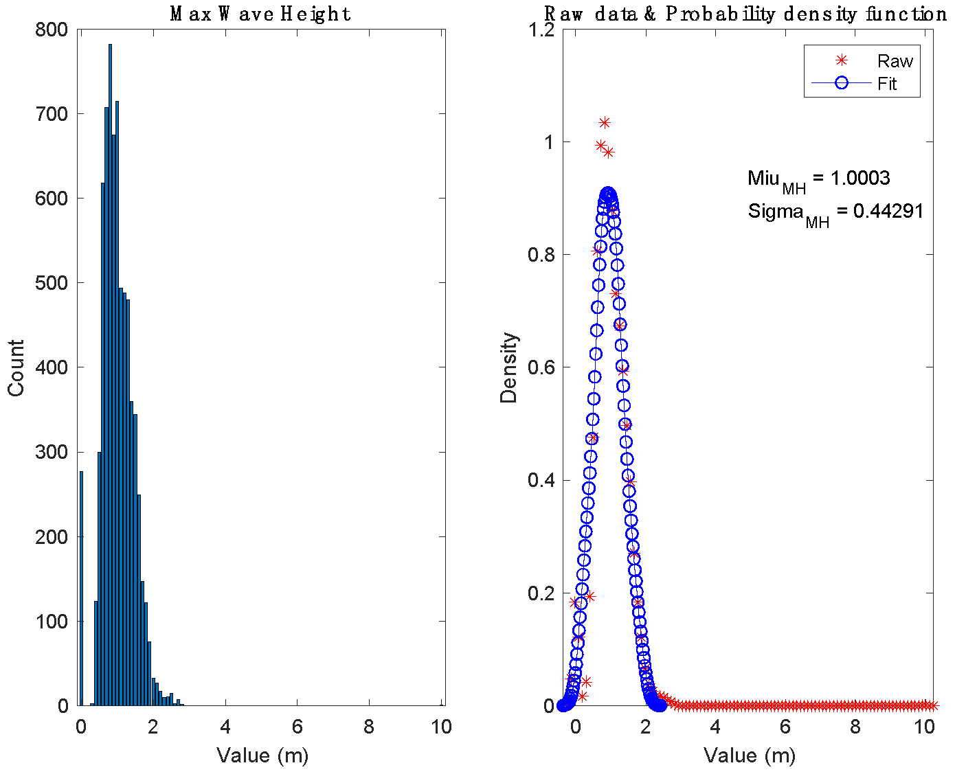
Figure 2.
Statistical compound current speed.
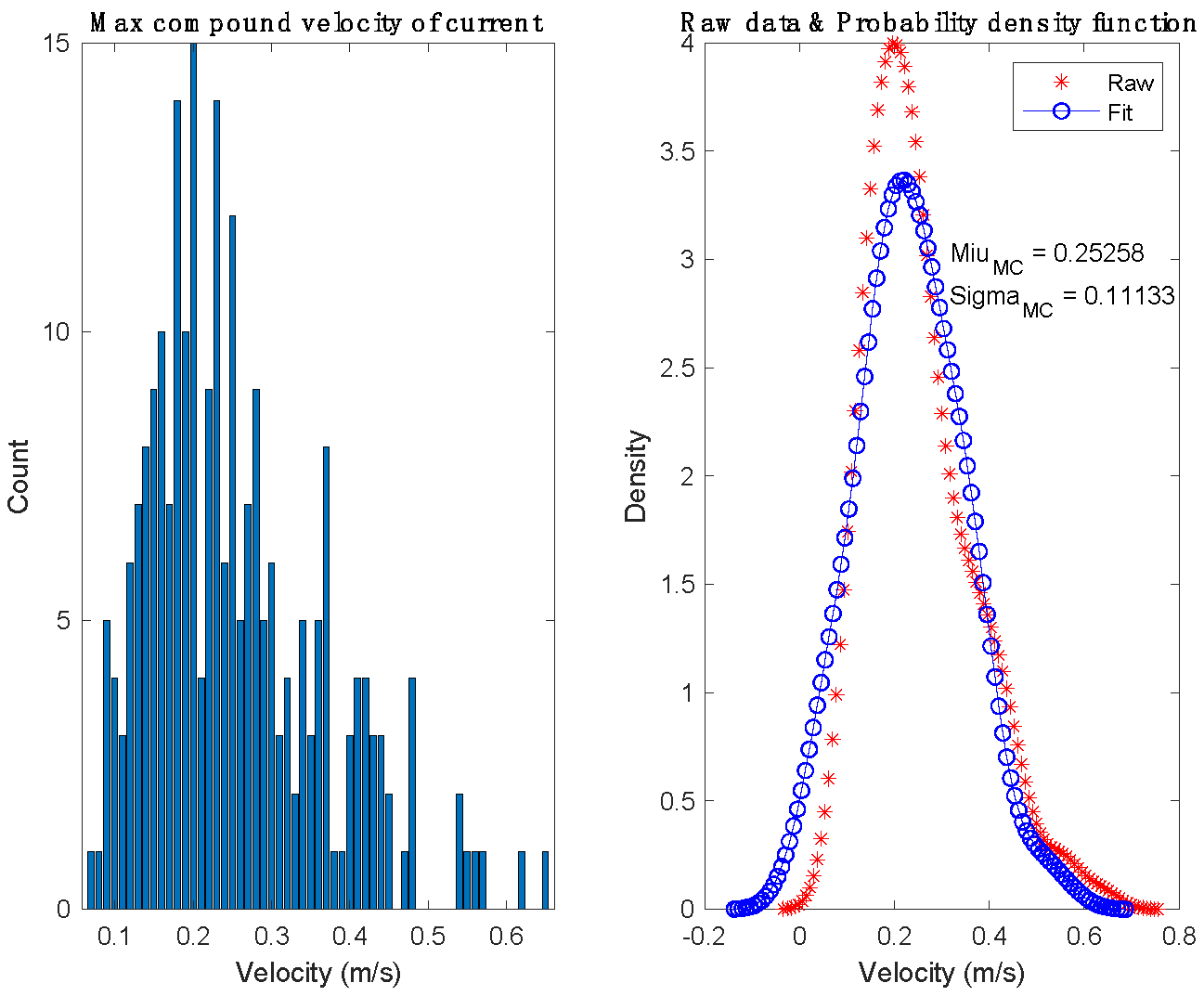
Figure 3.
Statistical compound wind speed.
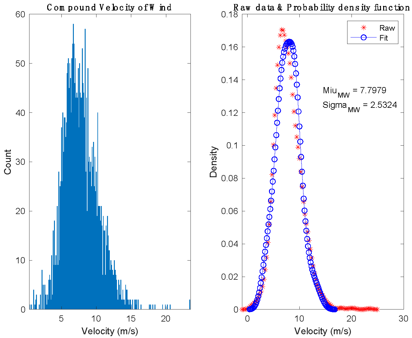
Figure 4.
Environment disturbance model.
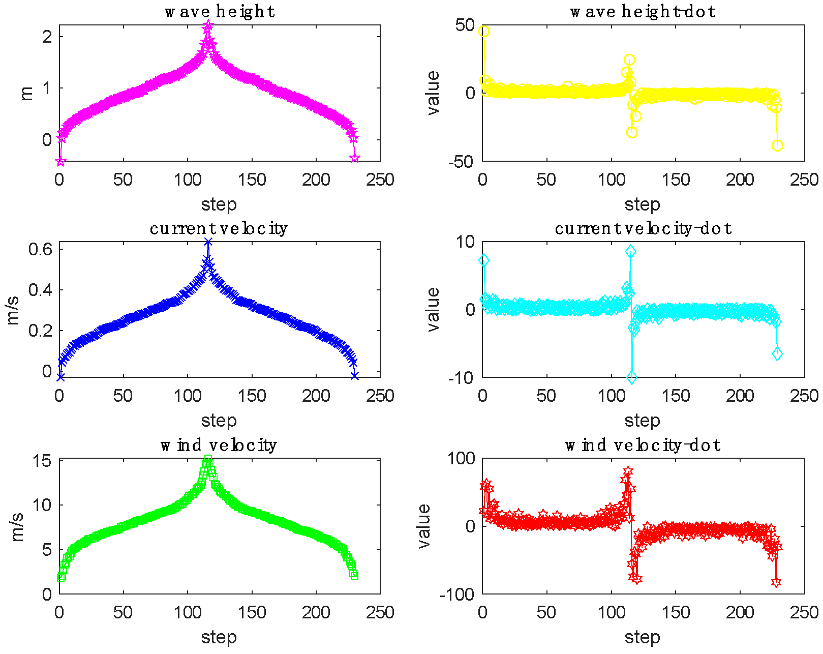
Figure 5.
Global coordinate frame E and body coordinate frame B.
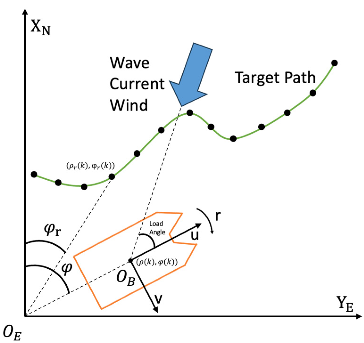
Figure 6.
No rudder angle with constant driving force, the impact of external disturbances.
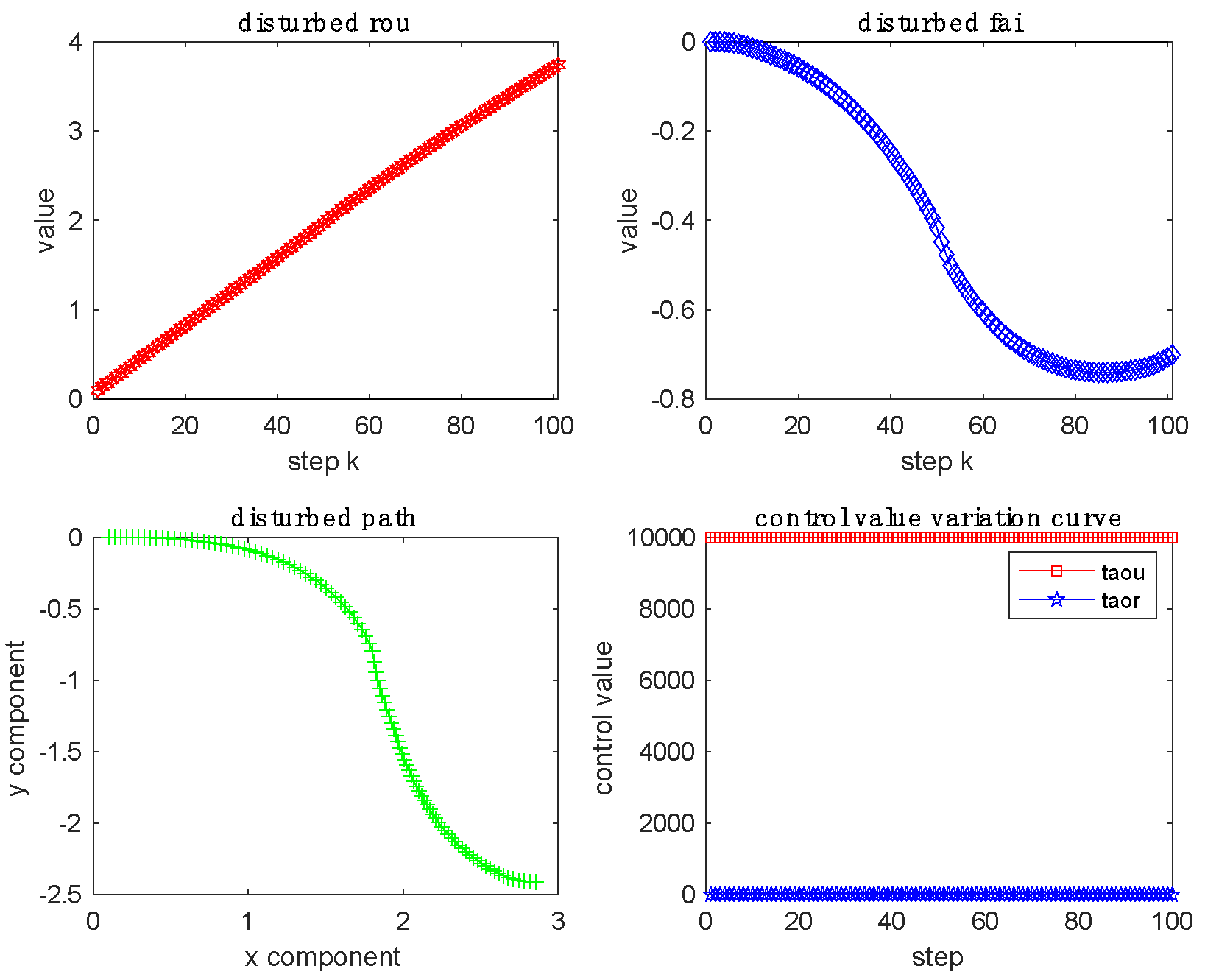
Figure 7.
No driving force with constant rudder angle, the effect of external disturbances.
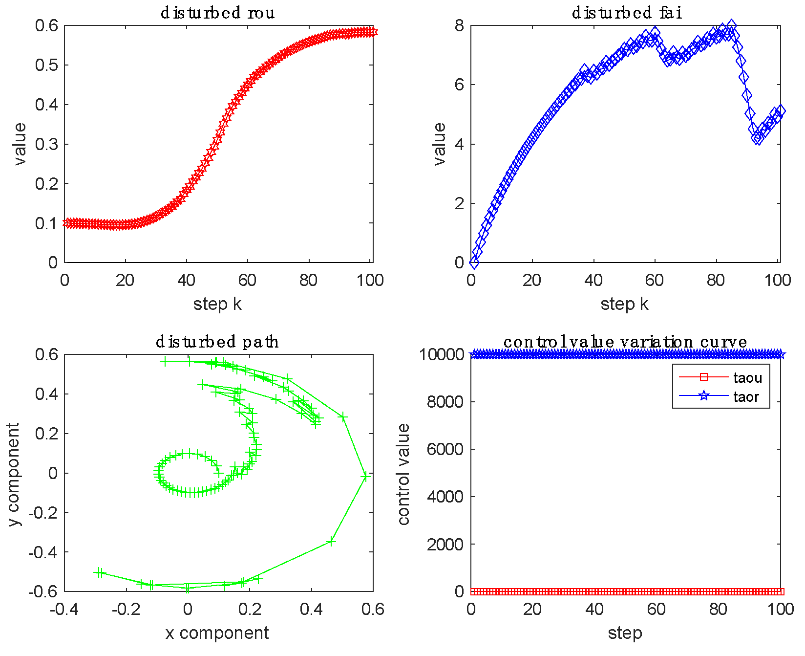
Figure 8.
Straight line path-tracking.
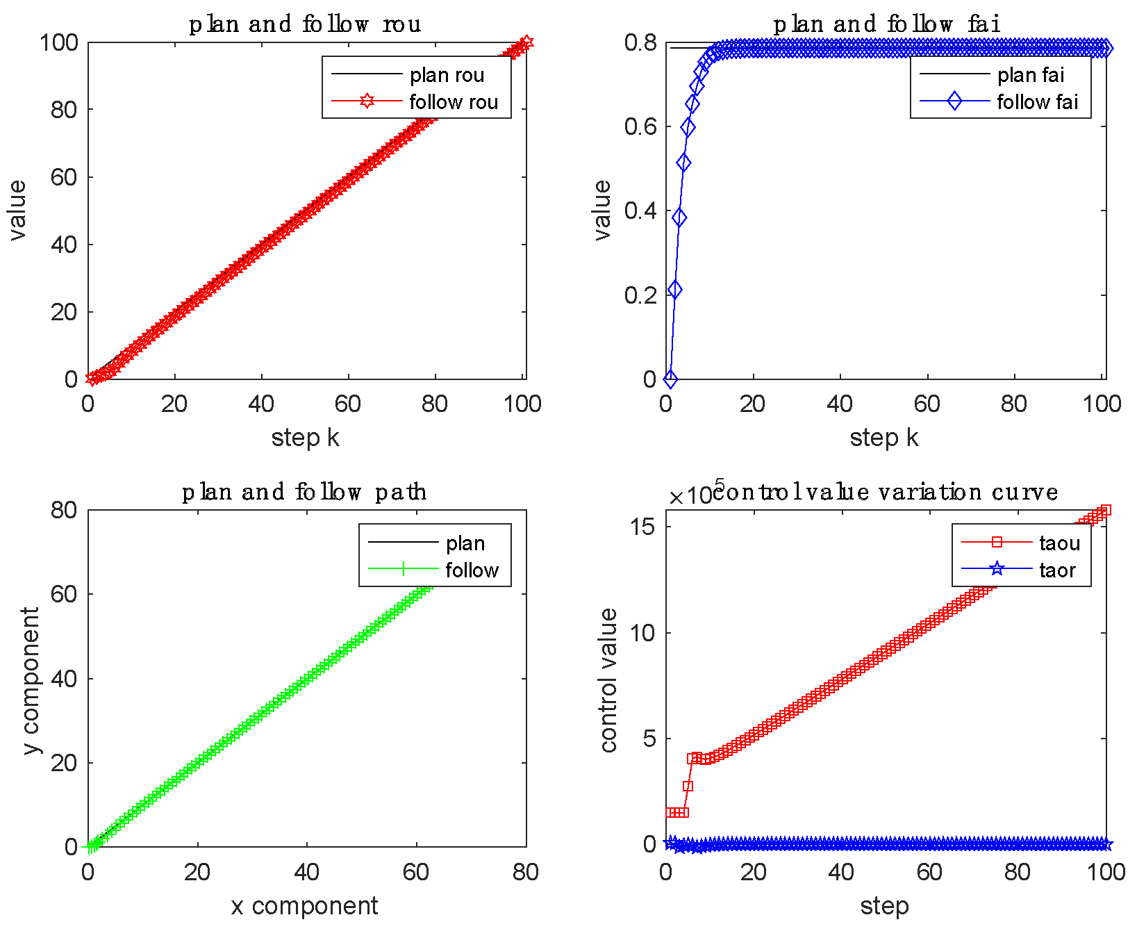
Figure 9.
Circular path-tracking.
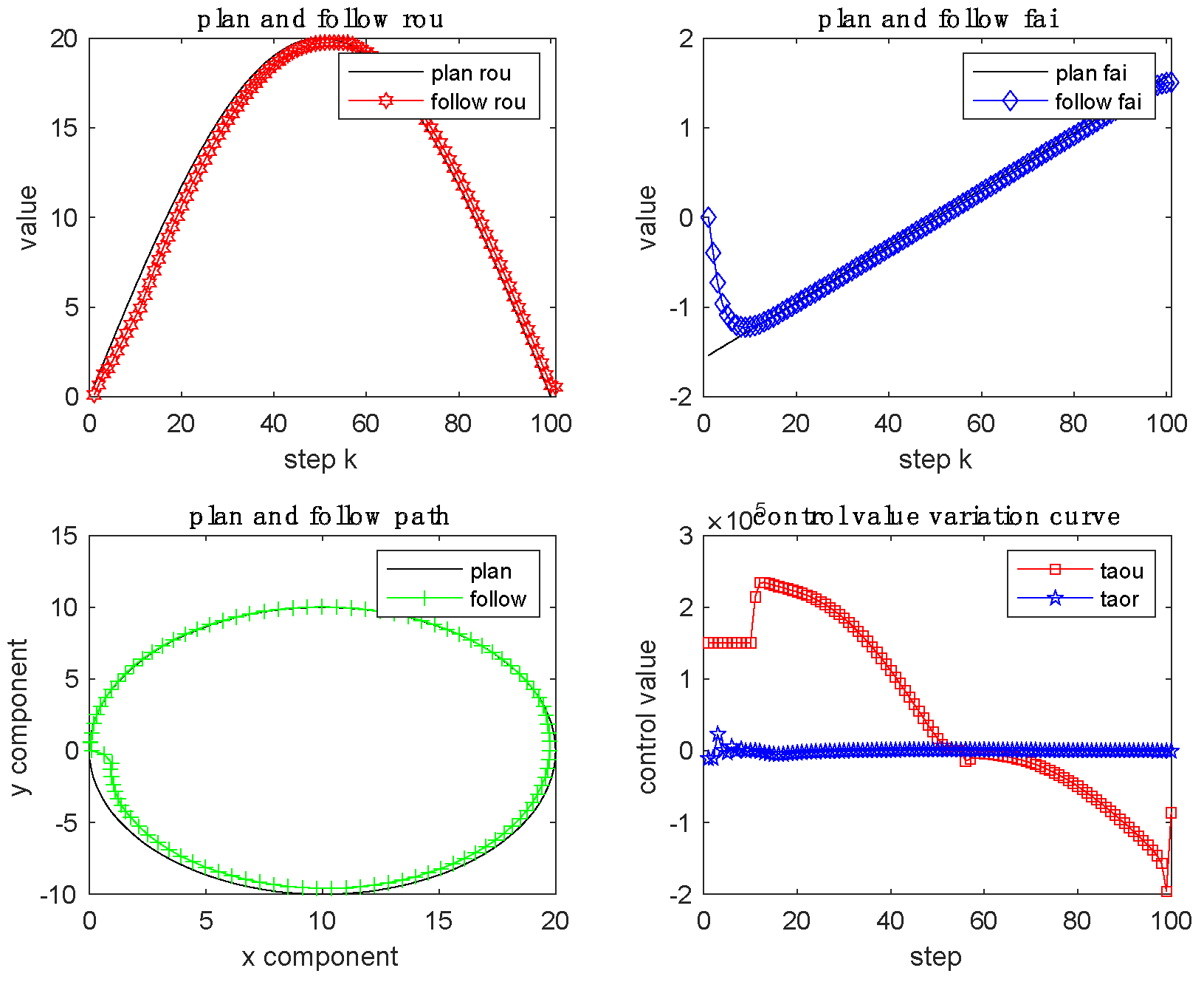
Figure 10.
Path-Tracking process of improved cost function in SMU-Smart Lake.
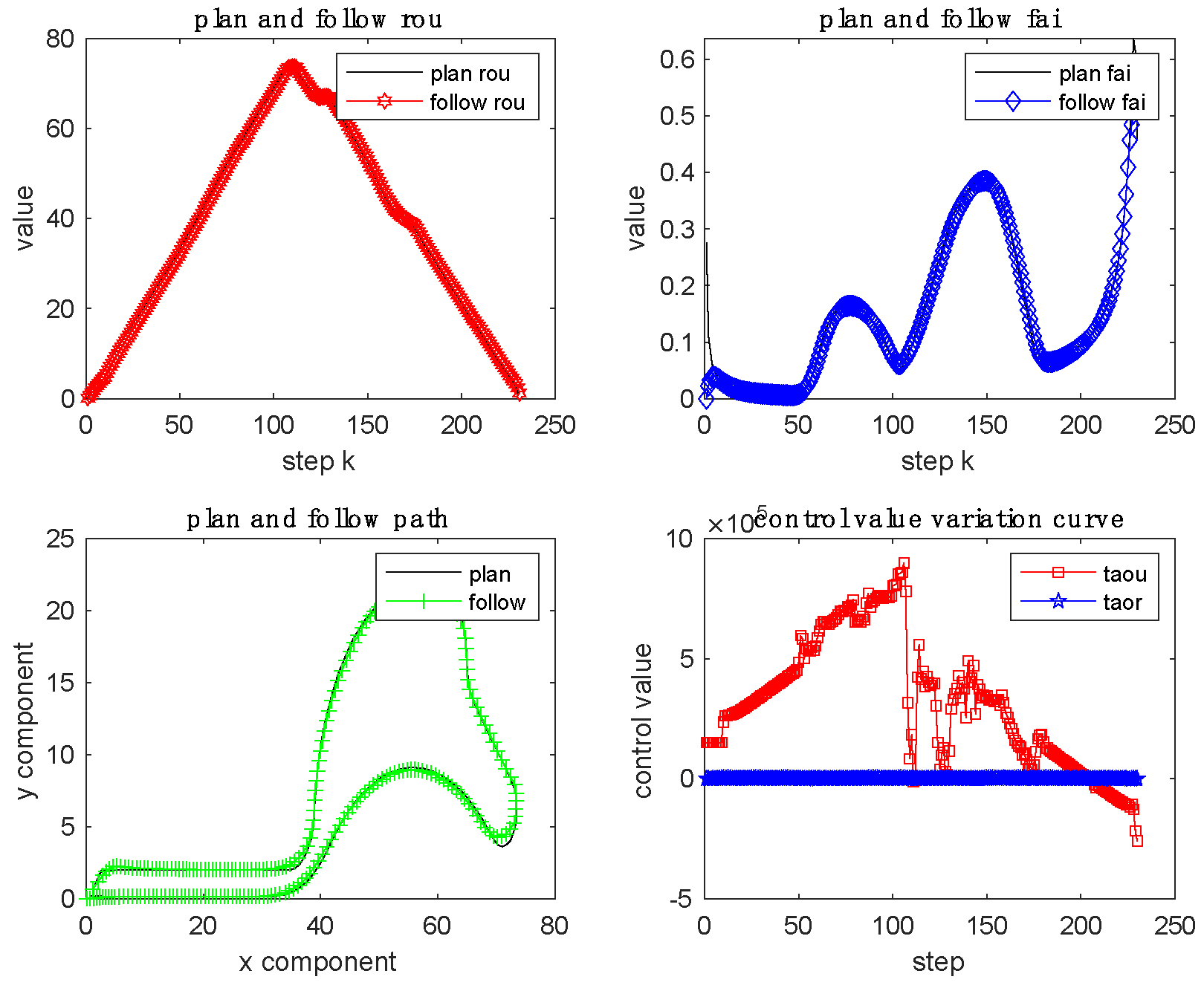
Figure 11.
Path-Tracking process of original cost function in SMU-Smart Lake.
Disclaimer/Publisher’s Note: The statements, opinions and data contained in all publications are solely those of the individual author(s) and contributor(s) and not of MDPI and/or the editor(s). MDPI and/or the editor(s) disclaim responsibility for any injury to people or property resulting from any ideas, methods, instructions or products referred to in the content. |
© 2023 by the authors. Licensee MDPI, Basel, Switzerland. This article is an open access article distributed under the terms and conditions of the Creative Commons Attribution (CC BY) license (http://creativecommons.org/licenses/by/4.0/).
Copyright: This open access article is published under a Creative Commons CC BY 4.0 license, which permit the free download, distribution, and reuse, provided that the author and preprint are cited in any reuse.


