
Submitted:
30 August 2024
Posted:
30 August 2024
You are already at the latest version
Abstract
An approach to estimate the dynamic characteristic of multilayered three-dimensional cubic quasicrystal cylindrical shells, annular plates, and truncated conical shells with different boundary conditions is presented. These investigated structures can be in a vacuum, totally filled with quiescent fluid, and subjected to internal flowing fluid, in which the fluid is incompressible and inviscid. The velocity potential, Bernoulli’s equation, and impermeability condition have been applied to the shell-fluid interface to obtain an explicit expression, from which the fluid pressure can be converted into the coupled differential equations in terms of displacement functions. The state-space method is formulated to quasicrystal linear elastic theory to derive the state equations for three structures along the radial direction. The mixed supported boundary conditions are represented by means of the differential quadrature technique and Fourier series expansions, respectively. A global propagator matrix, which connects the field variables at the internal interface to those at the external interface for the whole structure, is further completed by joint coupling matrices to overcome the numerical instabilities. Numerical examples show the correctness of the proposed method and the influence of the semi-vertical angle, different boundary conditions, and the fluid debit on the natural frequencies and mode shapes for various geometries and boundary conditions.
Keywords:
cubic quasicrystal materials
; truncated conical shells
; fluid-structure interaction
; fynamic analysis
1. Introduction
Multilayered structures in solid mechanics couple the performances of two different materials by means of the stacking sequence, adhesive, and intermetallic surface deposition. Different from crystal and amorphous materials, the ordered and quasi-periodic atomic arrangement of quasicrystals (QCs) materials enables them to exhibit some complex structures and special properties in theoretical analysis and experiments, especially their high stiffness-to-weight ratios, high resistivity, and excellent thermal-electro-elastic behaviors [1,2], which can be used to improve the structure performances of multilayered plates and shells. For optimal design and fabrication of the multilayered QC structures with desired properties, it is necessary to thoroughly understand the mechanical behaviors of multi-field coupled QC materials in complex environments. QC atomized powders were sprayed on steel substrates to evaluate the mechanical properties of QC coatings [3]. Meanwhile, Ferreira et al. [4] investigated the wear resistance and low friction of functionally graded aluminum at high temperatures, where the QC approximant phase played a critical role. The results show that the coated samples possessed high abrasion resistance, high micro-hardness, and excellent insulation. In addition, QC grains were developed into structural reinforcement phases and cast into alloys [5,6], from which the elongation, strength, and ductility of the specimens have been increased. Due to the mechanical properties of the multilayered composite structures being superior to those of components made of the individual material, they are tremendous applications in different engineering such as aerospace, medical devices, and semi-conductor.
To prevent the initiation and propagation of defects in the multilayered plate/shell model design, the vibrational frequencies and stress distributions of the multilayered cylindrical shells, truncated conical shells, and annular plates need to be accurately predicted and evaluated [7,8,9]. Ten different shell theories were adopted to derive the semi-analysis solutions of cylindrical shells, and numerical examples indicated that the results based on Soedel and Kennard-Simplified theories were more accurate than those compared to other theories [10]. Żur [11] presented the free vibration analysis of functionally graded circular plates with discrete elements by using the Neumann series method. Based on the discrete singular convolution method and differential quadrature method, Ersoy et al. [12] obtained the exact solutions of truncated conical shells, circular cylindrical shells, and annular plates. Eshaghi et al. [13] developed a numerical model of circular/annular plates under variable magnetic flux by using the Ritz method, from which the dynamic characteristics of the structure were obtained. Furthermore, they verified the effectiveness of this theoretical model in experiments. The free vibration problems of determining the field variables which occurred in functionally graded annular plates with general boundary conditions [14,15] have been derived, and the results showed that smaller gradient factors and elastic coefficients can retard the natural frequencies. Safarpour et al. [16] derived an exact solution of three-dimensional (3D) bending and frequency for functionally graded graphene platelet reinforced composite (FG-GPLRC) porous circular/annular plates with various boundary conditions. Meanwhile, the effects of geometric and material factors and different boundary conditions on the static and free vibration of FG-GPLRC were discussed using the theory of elasticity and differential quadrature method [17,18]. In addition, semi-analysis solutions of fiber metal annular plates with mixed boundary conditions [19] were developed to obtain the vibration frequencies. In the same way, truncated conical shells also have a wide range of engineering applications as the basic structure elements, and have attracted the tremendous attention of researchers. Kerboua and Lakis [20] obtained the free vibration analysis of discrete-continuous functionally graded circular plates via the Neumann series method. The first-order shell theory and the Sanders nonlinear kinematics equations [21] are proposed to investigate and improve the thermal and mechanical stability of functionally graded truncated conical shells.
In addition, the multi-physics phenomena between incompressible fluid flows and truncated conical shells may be encountered in practical engineering [22], such as oil transportation, urban pipe network laying, and fluid transmission. Izyan et al. [23] presented the numerical solutions and numerical examples of frequency parameters for truncated conical shells filled with quiescent fluid using Love’s first approximation theory. Based on the Mindlin thick shell theory, Hien et al. [24,25] derived the vibration responses of conical-cylindrical-conical shells containing fluid, and investigated the effect of fluid level, semi-vertex angles, and lamination sequences on three different joined cross-ply composite conical shells. Rahmanian et al. [26] obtained the natural frequencies of the coupled-field problem for multilayered truncated conical shells with different boundary conditions by using the same first-order shear deformation shell theory. In addition, for truncated conical shells with flowing liquid, Kerboua et al. [27] presented the explicit solution for fluid pressure according to Sanders’ thin shell theory, and the numerical results be used to present how the geometry, stress stiffening effect, and hydrodynamic effect of the combined application of internal fluid and external flow influence the dynamic behavior of the combined shell. The nonlinear shell theory along with Green’s strains was proposed to scrutinize the dynamic instabilities of the truncated conical shells subjected to flowing fluid [28], and some features showed that the appropriate dispersion of carbon nanotubes can improve the stability of the overall structure. In the literatures mentioned above, the various approximate plate and shell theories were employed to analyze the dynamic responses of these structures. However, these approximate theories may have certain assumptions and be easily affected by the thickness of the structure, resulting in numerical instability. In addition, the traditional propagator matrix method in these literatures cannot deal with the numerical instabilities in the case of large aspect ratios and high-order frequencies for QC plates/shells.
In this paper, the dynamic solutions of multilayered 3D cubic QC plates/shells subjected to flowing fluid are presented. Effects of different structure models, including the cylindrical shells, annular plates, and truncated conical shells, are taken into account. Governing equations of motion are derived in partial differential equation form by means of the state-space method. According to the differential quadrature (DQ) techniques and Fourier series expressions, the extra modifications to these state equations are performed to satisfy the different boundary conditions. The velocity potential and Bernoulli’s equations are implemented to determine pressures from quiescent or flowing fluids acting on the truncated conical shells. Different from the traditional propagator matrix method, the new propagator relation is reestablished to resolve numerical instabilities in the case of large aspect ratios and high-order frequencies for QC plates/shells. One numerical example is directed to shed light on the effectiveness of the presented method. Other numerical examples are obtained to analyze the influence of the semi-vertical angle, different boundary conditions, and the fluid debit on the natural frequencies and mode shapes for the QC plates/shells containing the quiescent or flowing inviscid fluid. In addition, these numerical results can be served as benchmarks for the design, numerical modeling, and simulation of the 3D cubic QC plates/shells.
2. Theoretical Formulation
As shown in Figure 1, a multilayered 3D cubic QC truncated conical shell composed of M layers with perfect bonding is considered, which has the length L = b – a, thickness h, and the semi-vertical angle α. Each layer has a thickness of hp = rp – rp-1, where rp-1 and rp denote the p-th of the inner and outer surfaces. It is clear that the inner and outer surfaces of this whole structure are r0 and rM, respectively. In a cylindrical coordinate system (r, θ, z), the mechanical behaviors of the cylindrical shell and annular plate can be obtained at the semi-vertical angles α = 0 and π/2, respectively.
2.1. Basic Equations
Based on the QC linear elasticity theory, the constitutive equations of 3D cubic QC materials [29,30] can be expressed as
where σmn and Hmn (m, n = r, θ, z) represent the stress components in phonon and phason fields, respectively. εmn and wmn denote the phonon and phason strains, respectively. C11, C12, and C44 are the phonon elastic constants, K11, K12, and K44 denote the phason elastic constants, and R1, R2, and R3 represent the phonon-phason elastic constants.
The relationship between the displacements and strains in phonon and phason fields [20,31] can be written as
where; um and wm represent the phonon and phason displacements, respectively.
The body forces are ignored and the equations of motion for truncated conical shell [23,29,32] containing fluid can be defined as
where p is the pressure exerted by the fluid on the shell wall; ρ denotes the mass density; t represents the time.
Based on the mixed formulation of solid mechanics, the state vector approach sets out-of-plane unknowns (ur, uθ, uz, wr, wθ, wz, σrr, σrθ, σrz, Hrr, Hrθ, Hrz) as basic variables, which are defined as primary variables A [33,34]. The state vector equations of the p-th layer can be established by combining the basic unknowns of three governing equations in Eqs. (1)-(3), which are expressed as
where the submatrices M1, M2, M3, and M4 in Eq. (4) can be found in Eqs. (A1)-(A4) of Appendix A, where some coefficients in Eqs. (A1)-(A4) and the following equations are listed in Eqs. (A5)-(A6).
The remaining stress components in Eq. (1) can be written as
The generalized displacement and stress solutions by the Fourier trigonometric expansions [35,36] are proposed to solve the partial differential equations of Eq. (4) in the θ-direction, as follows
where n is the half wavenumber in θ-direction; ω represents the angular frequency; i = .
It is difficult to deal with the partial differential equations of Eq. (4) in the z-direction, therefore, numerical manipulation, such as the DQ technique [37], is utilized to derive an exact solution for this problem. m th-order derivative of an unknown function f(z) [14,38] at discrete point i can be written as
whereare weight coefficients.
2.2. Modeling of the Fluid-Shell Interaction
The dynamic response of the QC truncated conical shell may be influenced tremendously when subjected to flowing liquid. This liquid filling model is based on the following hypotheses [20,27]: (i) the internal fluid is inviscid and incompressible; (ii) the fluid velocity is constant; (iii) the vibration is linear. Based on these assumptions, the velocity potential ϕ satisfying the Laplace equation [39] is written as
where ξ (0 ≤ ξ ≤ α) is designated as the coordinate along the α-direction.
The relationship between the velocity potential and fluid velocity can be expressed as
where V is the fluid velocity across a truncated conical shell section; and in the absence of the net flow rate of fluid, the fluid velocity components Vθ, Vz, and Vα can be written as
where Q is the fluid flowing with
in which Vave is the average fluid velocity.
In order to satisfy the impermeability condition between the truncated conical shell and internal fluid, the fluid velocity on the internal surface must be consistent with the instantaneous rate of change of displacement, as follows
with l = α – tan(h/2z).
Substituting Eq. (13) into Eq. (14), the impermeability condition can be rewritten as
where the superscript ‘′’ is the partial differentiation with respect to ξ. Then, combining Eq. (13) with Eq. (15), the representation of velocity potential ϕ is reestablished as
By plugging Eqs. (6) and (16) into Eq. (9), the function R(ξ) becomes
The solution of Eq. (17) can be derived by using the Frobenius method [23], as follows
where E is unknown.
Bernoulli's equation [20] for the pressure of the liquid on the shell wall is given by
where ρf denotes fluid density.
Applying Eq. (18) to Eq. (13) and then combining it with Eq. (19), the pressure p exerted by the fluid on the internal wall can be derived as
where k is a coefficient that is obtained from Eqs. (16) and (18). Applying the DQ method and Fourier trigonometric expansions into Eq. (20), the pressure p can be rewritten as
Thus, the first equation of motion in Eq. (3) is related to phonon stresses and pressure.
2.3. Dispersion of State-Space Equations
The stresses and displacements in the θ-direction and z-direction are expressed in terms of Fourier trigonometric expansions and DQ regional discrete point expansions, respectively, from which the partial differential state equations in Eq. (4) can be converted into ordinary differential equations, as follows
where, in which the superscript ‘T’ represents the matrix or vector transpose; The superscript ‘p’ represents the state variables or coefficient matrix of the p-th layer. The submatrices T1, T2, T3, and T4 of the coefficient matrix T can be found in Eqs. (A7)-(A10) of Appendix A.
Similarly, Eq. (5) can be processed by Fourier trigonometric expansions and the DQ technique. In this paper, simple supported (S) and clamped supported (C) boundary conditions are considered for multilayered cubic QC truncated conical shells. The mechanical boundary conditions at z = a and b can be written as [40]
For example, ‘CS’ denotes a shell with the clamped supported and simple supported boundary conditions at z = a and b, respectively. The semi-analysis solutions of QC truncated conical shells with four kinds of boundary conditions (SS, CS, SC, and CC) are obtained and the coefficients matrices of state equations for shells with CS boundary conditions are listed in Eqs. (A13)-(A16) of Appendix A.
2.4. Vibration Analysis
Based on the theory of ordinary differential equations, the matrix exponential method can be utilized to derive the solution of Eq. (22) [41], as follows
Let r = rp in Eq. (25), this equation is in the following form
Eq. (26) can be rewritten as
where the superscripts ‘+’ and ‘−’ are defined as variables on the upper surface and the lower surface of the p-th layer, respectively.
It is assumed that the field variables are assumed to be continuous through the interface rp, as follows
According to the continuity interface conditions of rp, Eq. (28) can be redefined as
where= [I, −I] is the joint coupling matrix at the interface rp.
Similarly, the interface relationship of the top and bottom surfaces for the QC truncated conical shell is
where Jt= Jw= [I, 0].
Combining Eqs. (29) with (30), the interface condition of the integral shell is
where
The whole structure can be defined in the same form as Eq. (31), as follows
where
Substituting Eq. (33) into Eq. (31) results in
Eq. (35) can be rewritten as
By solving Eq. (36), the vibration solutions of the whole multilayered QC structure are obtained.
3. Numerical Results and Discussion
Illustrative examples of the state-space based differential quadrature method (SS-DQM) of the multi-physics problems between incompressible fluid flows and truncated conical shells are presented. The aspect ratios for these structures are set as a/b = 0.4 and h/b = 0.03. The cylindrical shells, annular plates, and truncated conical shells are composed of two 3D cubic QC materials, and they are abbreviated as QC1 and QC2. Meanwhile, the material properties [1,29] of the constituents are listed in Table 1, and these material coefficients completely match the elastic deformation energy density of the QC materials and satisfy the positive definiteness of the QC materials [42,43]. The structure (called QC1/QC2/QC1), composed of three single layers of the same thickness, is taken in the following text. The half wavenumber in Eq. (6) is taken as n = 1, and the discrete point is set to N = 13. In addition, the dimensionless quantities [44] are employed
where Cmax and ρmax denote the maximum values of the phonon elastic constant and mass density for QC multilayered structures, respectively.
3.1. Convergence and Validation Studies
To prove the formula and program in this paper, the numerical results of the QC model by the proposed method are compared with those by the state-space method (SSM) [33]. The first seven order dimensionless natural frequencies Ω of the QC cylindrical shells (α = 0) with boundary conditions SS are presented in Table 2. It is noted that the first five order modes are the flexural frequencies, but Modes 6 and 7 are longitudinal frequencies. The maximal relative error of the frequencies values Ω obtained from the present and SSM is less than 0.01%.
Similarly, Figure 2 shows that the variations of the first order normalized mode shapes of the displacements and stresses along the r-direction are obtained using the present method and SSM. The distributions of ur and wr are flexural mode shapes. The results obtained by the two methods are consistent. This feature indicates that the method in this paper has high precision and good convergence and the solutions are stable. As mentioned in the introduction, research works for the vibration analysis of the empty and fluid-filled QC conical shells are encountered less frequently. because cylindrical shells can be viewed as a special case of conical vessels with equal top and bottom radii, both Ω and mode shapes are good consistent by using the present method and SSM, which can be used as an example to verify the correctness of formulas and procedures for QC conical shells.
To ensure that the present method is valid and accurate, a 3D cubic QC sandwich plate with simply supported boundary conditions is considered. The material coefficients, the shape and size, and the expression form of field variables are consistent with those in Ref. [29]. In addition, the interface coefficient is taken as δ = 0. The numerical results for the QC1/QC2/QC1 plate are calculated by using SS-DQM to compare with the results presented in Figure 6 (a)-(d) of Ref. [29]. The first five order dimensionless natural frequencies Ω of the QC plate are presented in Table 3. Meanwhile, Figure 2 (b) presents the variation of the phonon and phason displacements ux, wx, uz, and wz. The obtained solutions for Ω and normalized displacement mode shapes by using SS-DQM are in good agreement with the results of Ref. [29] by using pseudo-Stroh formalism. Thus, the method in this paper has high precision and good convergence.
3.2. QC Annular Plates with Different Boundary Conditions
In this part, the solutions of the QC annular plates (α = π/2) with the boundary conditions SS, CS, SC, and CC are presented. The first nine order dimensionless natural frequencies Ω of the QC annular plates without fluid are presented in Table 4 to show the effect of the simple supported and clamped supported boundary conditions on Ω. Every order Ω increases in the order of SS, CS, SC, and CC for a fixed value of h/L. Different from QC cylindrical shells with the boundary condition SS, Modes 1, 2, 3, 5, 7, and 9 of QC annular plates are the flexural frequencies, but Modes 4, 6, and 8 are longitudinal frequencies.
The radial coordinates of data points in the resulting graph of this section are fixed at z/b = 0.7. The ring coordinates of data points are all basic solutions, and the angle variation can be multiplied by the sine-cosine factor from Eq. (6). Figure 3 shows the variations of the first-order mode shapes of the phonon and phason displacements for QC annular plates with four different boundary conditions along the r-direction. The distributions of and (Figure 3 (a) and (c)) are symmetrical, but the distributions of and (Figure 3 (b) and (d)) is anti-symmetrical at r/b = 0.045, so these curves are flexural mode shapes. Moreover, the values of the mode shapes for and at r/b = 0.03 and 0.06 decrease in the order of SC, CC, SS, and CS for a fixed value of h/L. In addition, observing that the phason mode shapes and are sensitive to the different boundary conditions.
Figure 4 shows the variations of the first-order mode shapes of the phonon and phason stresses for QC annular plates with four different boundary conditions along the r-direction. (Figure 4 (a)) of QC annular plates with boundary conditions CS and CC experience a large slope jump at the two interfaces based on the QC linear elastic theory. Besides that, increasing the phonon material properties of QC2 helps reduce this jump. (Figure 4 (b)) of the plates with boundary conditions CS exhibits a different response from plates with other boundary conditions. The maximal values of and (Figure 4 (c) and (d)) at r/b = 0.03 and 0.06 increase in the order of SS, SC, CS, and CC for a fixed value of h/L. These features show that the clamped boundary condition increases the stiffness of the plate, resulting in changes in frequencies and mode shapes.
3.3. Dynamic Behavior of the Empty and Fluid-Filled Shell
In this part, the solutions of the QC truncated conical shells with quiescent fluid are presented. The first five order dimensionless natural frequencies Ω of the QC shells with boundary condition SS are listed in Table 5, in which α0 is defined as the shell without fluid. The natural frequencies Ω of shells containing quiescent fluid are greater than that of the shell without fluid at the same α. This feature shows that quiescent fluid improves the overall stiffness of these shells. Meanwhile, as α increases, Ω decreases except for mode 4. This indicates that the device composed of QC truncated conical shells would be more susceptible to external motivation with α increasing. In other words, the QC structures with large α are more likely to cause structural resonance under external motivation.
The contour plots of the dimensionless phonon displacement mode shapes and for QC truncated conical shells on the r-z plane are presented in Figure 5 and Figure 6. The distributions of (Figure 5 (a)-(d)) for QC shell are all asymmetrical at z/b = 0.7 mm and almost constant along the r-direction. The maximum value of becomes greater with α increases. Results in Figure 5 and Figure 6 confirm that the phonon displacement boundary conditions in Eq. (27) are precisely satisfied, partially verifying the accuracy of the present methods. The distributions of (Figure 6 (a)-(d)) is nonlinear, from which the first-order, second-order, and higher-order plate and shell theories are imprecise.
Figure 5.
The contour plots of the phonon displacement mode shape (10-2): (a) α0 = π/6, (b) α = π/6, (c) α = π/4, and (d) α = π/3.
Figure 5.
The contour plots of the phonon displacement mode shape (10-2): (a) α0 = π/6, (b) α = π/6, (c) α = π/4, and (d) α = π/3.
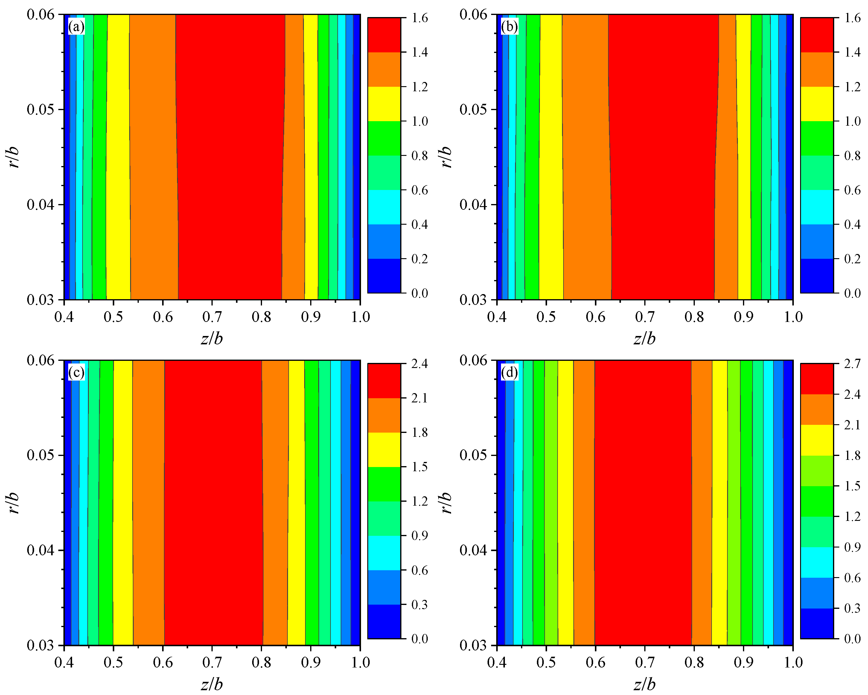
Figure 6.
The contour plots of the phonon displacement mode shape (10-3): (a) α0 = π/6, (b) α = π/6, (c) α = π/4, and (d) α = π/3.
Figure 6.
The contour plots of the phonon displacement mode shape (10-3): (a) α0 = π/6, (b) α = π/6, (c) α = π/4, and (d) α = π/3.

In r-z plane distributions of the dimensionless phason displacement mode shapes and for QC truncated conical shells are plotted in Figure 7 and Figure 8. (Figure 7 (a)-(d)) experiences a large slope jump in the r-z plane for the classical elasticity case and increasing α changes the direction of the jump. It is seen that the distribution of in Figure 8 (a)-(d) is of the polygonal line while that of is not, and and show different behaviors in the r-z plane. This difference is mainly due to differences in material properties since the two in-plane mode shapes of the QC shell should have the same distribution curves in a physical sense. and remain continuous at the interfaces at r/b = 0.04 and 0.05. The distributions of and are similar in the r-z plane. This feature indicates that the phonon and phason elementary excitations in QCs both need to be analyzed.
3.4. QC Truncated Conical Shells Containing Flowing Fluid
In this part, the solutions of interaction between incompressible fluid flow and QC truncated conical shells with boundary conditions CS are presented. The centrifugal, Coriolis, and inertial forces will affect the stability of the whole structure when the incompressible fluid is flowing through the shell. The material and physical properties of the whole model are α = π/12 and ρf = 1000 kg/m3. The first five order dimensionless natural frequencies Ω of the QC shells with different fluid debits Q are listed in Table 6. These frequencies Ω are increased by increasing the mean fluid velocity due to Q being a constant related to the flow rate. Meanwhile, these Ω show that the model composed of fluid flow and QC shells can be obtained accurately calculate at a small α.
Figure 9 and Figure 10 show the variation of the first-order dimensionless displacement and stress mode shapes of QC truncated conical shells with different Q, respectively. An increase in Q results in a decrease in the magnitude of and (Figure 9 (a) and (b)) for QC shells. The decreasing of the values of the mode shapes is fast in the range of 1 m3/s ≤ Q ≤ 2 m3/s. It is noted that and are continuous across the interfaces for the classical elasticity case. However, (Figure 9 (c)) shows different behavior, especially in the middle layers of the QC shell. experience a slope jump at r/b = 0.04 and 0.05. In addition, Q has little effect on (Figure 9 (d)), including , and . The maximum values of and (Figure 10 (a) and (c)) occur at the interfaces between layers. Different from the distribution of , (Figure 10 (b)) is insensitive to Q. Similarly, (Figure 10 (d)) is as insensitive to Q as the phason displacement mode shapes. This feature shows the weak coupling between phason and velocity potential.
4. Conclusions
This paper presents a semi-analysis method to evaluate the natural frequencies and mode shapes of 3D cubic QC cylindrical shells, annular plates, and truncated conical shells under vacuum and fluid. Since no assumptions on stresses and displacements have been employed, the present framework can be applied to an arbitrary thickness of plate/shell structures. Some significant features are listed below.
- The global propagator relation is reestablished to resolve numerical instabilities in the case of large discrete point numbers and high frequencies for three QC structures. Some cases such as one-dimensional and two-dimensional QC plates/shells could all be investigated according to the present methods.
- Quiescent fluid improves the overall stiffness of the truncated conical shell. This shell with the higher semi-vertical angle α leads to smaller natural frequencies and phonon displacements mode shapes and larger phason displacements mode shapes. Meanwhile, QC truncated conical shells are more susceptible to external excitation with semi-vertical angle α increasing
- Every order of natural frequencies increases in the order of SS, CS, SC, and CC for a fixed value of h/L. Higher fluid debits Q causes shells to experience larger frequencies in the case of all boundary conditions. All phason variables are insensitive to fluid debits Q.
The methods and numerical results in this paper can be utilized to validate the accuracy of other numerical methods and serve for the analysis and design of intelligent QC material plates/shells.
Acknowledgments
Funding: This work was supported by the National Natural Science Foundation of China
[grant numbers 11972365 and 12272402] and the China Agricultural University Education Foundation [grant numbers 1101‐240001].
Appendix A
The submatrices M1, M2, M3, and M4 in Eq. (4) are
The coefficients of Eqs. (A1)-(A4) can be found in Eqs. (A5) and (A6), as follows
The submatrices T1, T2, T3, and T4 in Eq. (22) are defined as
where
with
The coefficients matrices of state equations for shells with CS boundary conditions are expressed as
where
References
- Fan T Y. Mathematical theory of elasticity of quasicrystals and its applications[M]. Heidelberg: Springer, 2011.
- Li X F. Elastohydrodynamic problems in quasicrystal elasticity theory and wave propagation[J]. Philosophical Magazine, 2013, 93(13): 1500-1519. [CrossRef]
- Wolf W, Schulz R, Savoie S, et al. Structural, mechanical and thermal characterization of an Al-Co-Fe-Cr alloy for wear and thermal barrier coating applications[J]. Surface Coatings Technology, 2017, 319: 241-248. [CrossRef]
- Ferreira T, Koga G Y, De Oliveira I L, et al. Functionally graded aluminum reinforced with quasicrystal approximant phases - Improving the wear resistance at high temperatures[J]. Wear, 2020, 462: 203507. [CrossRef]
- Zhang X J, Wang H W, Yan B, et al. The nanoscale strain assignment behavior of icosahedral quasicrystalline phase T2-Al6CuLi3 in cast Al-Li alloys[J]. Journal of Alloys and Compounds, 2021, 867(6): 159096. [CrossRef]
- Guo J H, Liu G T. Analytic solutions to problem of elliptic hole with two straight cracks in one-dimensional hexagonal quasicrystals[J]. Applied Mathematics and Mechanics-English Edition, 2008, 29(4): 485-493. [CrossRef]
- Sun T Y, Guo J H, Pan E. Nonlocal vibration and buckling of two-dimensional layered quasicrystal nanoplates embedded in an elastic medium[J]. Applied Mathematics and Mechanics, 2021, 42(8): 1077-1094. [CrossRef]
- Ye J Q. Laminated composite plates and shells: 3D modelling[M]. Springer Science and Business Media, 2002.
- Vattré A, Pan E. Thermoelasticity of multilayered plates with imperfect interfaces[J]. International Journal of Engineering Science, 2021, 158: 103409. [CrossRef]
- Farshidianfar A, Oliazadeh P. Free vibration analysis of circular cylindrical shells: comparison of different shell theories[J]. International Journal of Mechanics Applications, 2012, 2(5): 74-80.
- Żur K K. Free vibration analysis of discrete-continuous functionally graded circular plate via the Neumann series method[J]. Applied Mathematical Modelling, 2019, 73: 166-189. [CrossRef]
- Ersoy H, Mercan K, Civalek Ö. Frequencies of FGM shells and annular plates by the methods of discrete singular convolution and differential quadrature methods[J]. Composite Structures, 2018, 183: 7-20. [CrossRef]
- Eshaghi M, Sedaghati R, Rakheja S. Analytical and experimental free vibration analysis of multi-layer MR-fluid circular plates under varying magnetic flux[J]. Composite Structures, 2016, 157: 78-86. [CrossRef]
- Yas M H, Jodaei A, Irandoust S, et al. Three-dimensional free vibration analysis of functionally graded piezoelectric annular plates on elastic foundations[J]. Meccanica, 2011, 47(6): 1401-1423. [CrossRef]
- Yas M H, Moloudi N. Three-dimensional free vibration analysis of multi-directional functionally graded piezoelectric annular plates on elastic foundations via state space based differential quadrature method[J]. Applied Mathematics and Mechanics, 2015, 36(4): 439-464. [CrossRef]
- Safarpour M, Rahimi A, Alibeigloo A, et al. Parametric study of three-dimensional bending and frequency of FG-GPLRC porous circular and annular plates on different boundary conditions[J]. Mechanics Based Design of Structures and Machines, 2021, 49(5): 707-737. [CrossRef]
- Rahimi A, Alibeigloo A, Safarpour M. Three-dimensional static and free vibration analysis of graphene platelet–reinforced porous composite cylindrical shell[J]. Journal of Vibration and Control, 2020, 26(19-20): 1627-1645. [CrossRef]
- Safarpour M, Rahimi A R, Alibeigloo A. Static and free vibration analysis of graphene platelets reinforced composite truncated conical shell, cylindrical shell, and annular plate using theory of elasticity and DQM[J]. Mechanics Based Design of Structures and Machines, 2020, 48(4): 496-524. [CrossRef]
- Rahimi G H, Gazor M S, Hemmatnezhad M, et al. Free vibration analysis of fiber metal laminate annular plate by state-space based differential quadrature method[J]. Advances in Materials Science Engineering, 2014, 2014(3): 653-659. [CrossRef]
- Kerboua Y, Lakis A A. Numerical model to analyze the aerodynamic behavior of a combined conical–cylindrical shell[J]. Aerospace Science and Technology, 2016, 58: 601-617. [CrossRef]
- Naj R, Sabzikar Boroujerdy M, Eslami M R. Thermal and mechanical instability of functionally graded truncated conical shells[J]. Thin-Walled Structures, 2008, 46(1): 65-78. [CrossRef]
- Jooybar N, Malekzadeh P, Fiouz A, et al. Thermal effect on free vibration of functionally graded truncated conical shell panels[J]. Thin-Walled Structures, 2016, 103: 45-61. [CrossRef]
- Izyan M D N, Viswanathan K K, Aziz Z A, et al. Free vibration of layered truncated conical shells filled with quiescent fluid using spline method[J]. Composite Structures, 2017, 163: 385-398. [CrossRef]
- Hien V Q, Thinh T I, Cuong N M, et al. Free vibration analysis of joined composite conical-conical-conical shells containing fluid[J]. Vietnam Journal of Science echnology, 2016, 54(5): 650. [CrossRef]
- Hien V Q, Thinh T I, Cuong N M. Free vibration analysis of joined composite conical-cylindrical-conical shells containing fluid[J]. Vietnam Journal of Mechanics, 2016, 38(4): 249-265. [CrossRef]
- Rahmanian M, Firouz-Abadi R D, Cigeroglu E. Free vibrations of moderately thick truncated conical shells filled with quiescent fluid[J]. Journal of fluids structures, 2016, 63: 280-301. [CrossRef]
- Kerboua Y, Lakis A A, Hmila M. Vibration analysis of truncated conical shells subjected to flowing fluid[J]. Applied Mathematical Modelling, 2010, 34(3): 791-809. [CrossRef]
- Mohammadi N, Asadi H, Aghdam M M. An efficient solver for fully coupled solution of interaction between incompressible fluid flow and nanocomposite truncated conical shells[J]. Computer Methods in Applied Mechanics and Engineering, 2019, 351: 478-500. [CrossRef]
- Feng X, Fan X Y, Li Y, et al. Static response and free vibration analysis for cubic quasicrystal laminates with imperfect interfaces[J]. European Journal of Mechanics - A/Solids, 2021, 90(14): 104365. [CrossRef]
- Li X Y. Fundamental solutions of penny-shaped and half-infinite plane cracks embedded in an infinite space of one-dimensional hexagonal quasi-crystal under thermal loading[J]. Proceedings of the Royal Society A: Mathematical, Physical and Engineering Sciences, 2013, 469(2154): 20130023. [CrossRef]
- Huang Y Z, Li Y, Zhang L L, et al. Dynamic analysis of a multilayered piezoelectric two-dimensional quasicrystal cylindrical shell filled with compressible fluid using the state-space approach[J]. Acta Mechanica, 2020, 231(6): 2351-2368. [CrossRef]
- Li X Y, Wang T, Zheng R F, et al. Fundamental thermo-electro-elastic solutions for 1D hexagonal QC[J]. ZAMM - Journal of Applied Mathematics and Mechanics / Zeitschrift für Angewandte Mathematik und Mechanik, 2015, 95(5): 457-468. [CrossRef]
- Huang Y Z, Li Y, Yang L Z, et al. Static response of functionally graded multilayered one-dimensional hexagonal piezoelectric quasicrystal plates using the state vector approach[J]. Journal of Zhejiang University-Science A, 2019, 20(2): 133-147.
- Li Y, Li Y, Qin Q H, et al. Axisymmetric bending analysis of functionally graded one-dimensional hexagonal piezoelectric quasi-crystal circular plate[J]. Proceedings of the Royal Society A, 2020, 476(2241): 20200301. [CrossRef]
- Chen J Y, Guo J H, Pan E. Wave propagation in magneto-electro-elastic multilayered plates with nonlocal effect[J]. Journal of Sound and Vibration, 2017, 400: 550-563. [CrossRef]
- Vattré A, Pan E, Chiaruttini V. Free vibration of fully coupled thermoelastic multilayered composites with imperfect interfaces[J]. Composite Structures, 2021, 259: 113203. [CrossRef]
- Bellman R, Kashef B G, Casti J. Differential quadrature: A technique for the rapid solution of nonlinear partial differential equations[J]. Journal of Computational Physics, 1972, 10(1): 40-52. [CrossRef]
- Lü C F, Chen W Q, Shao J W. Semi-analytical three-dimensional elasticity solutions for generally laminated composite plates[J]. European Journal of Mechanics - A/Solids, 2008, 27(5): 899-917. [CrossRef]
- Korn G A, Korn T M. Mathematical handbook for scientists and engineers: definitions, theorems, and formulas for reference and review[M]. Courier Corporation, 2000.
- Yan W W, Xu M Z. Dependence of eigenvalues of second-order differential operator with eigen parameters contained in both boundary conditions[J]. Journal of Inner Mongolia University of Technology(Natural Science Edition), 2022, 41(14): 294-300.
- Chen W Q, Cai J B, Ye G R. Exact solutions of cross-ply laminates with bonding imperfections[J]. Aiaa Journal, 2003, 41(11): 2244-2250. [CrossRef]
- Hwu C. Anisotropic Elastic Plates[M]. Spring Science and Business Media, 2010.
- Hu C Z, Wang R H, Ding D H. Symmetry groups, physical property tensors, elasticity and dislocations in quasicrystals[J]. Reports on Progress in Physics, 2000, 63(1): 1-39. [CrossRef]
- Wu D, Zhang L L, Xu W S, et al. Electroelastic Green's function of one-dimensional piezoelectric quasicrystals subjected to multi-physics loads[J]. Journal of Intelligent Material Systems and Structures, 2017, 28(12): 1651-1661. [CrossRef]
Figure 1.
Geometry and layout of a truncated conical shell.
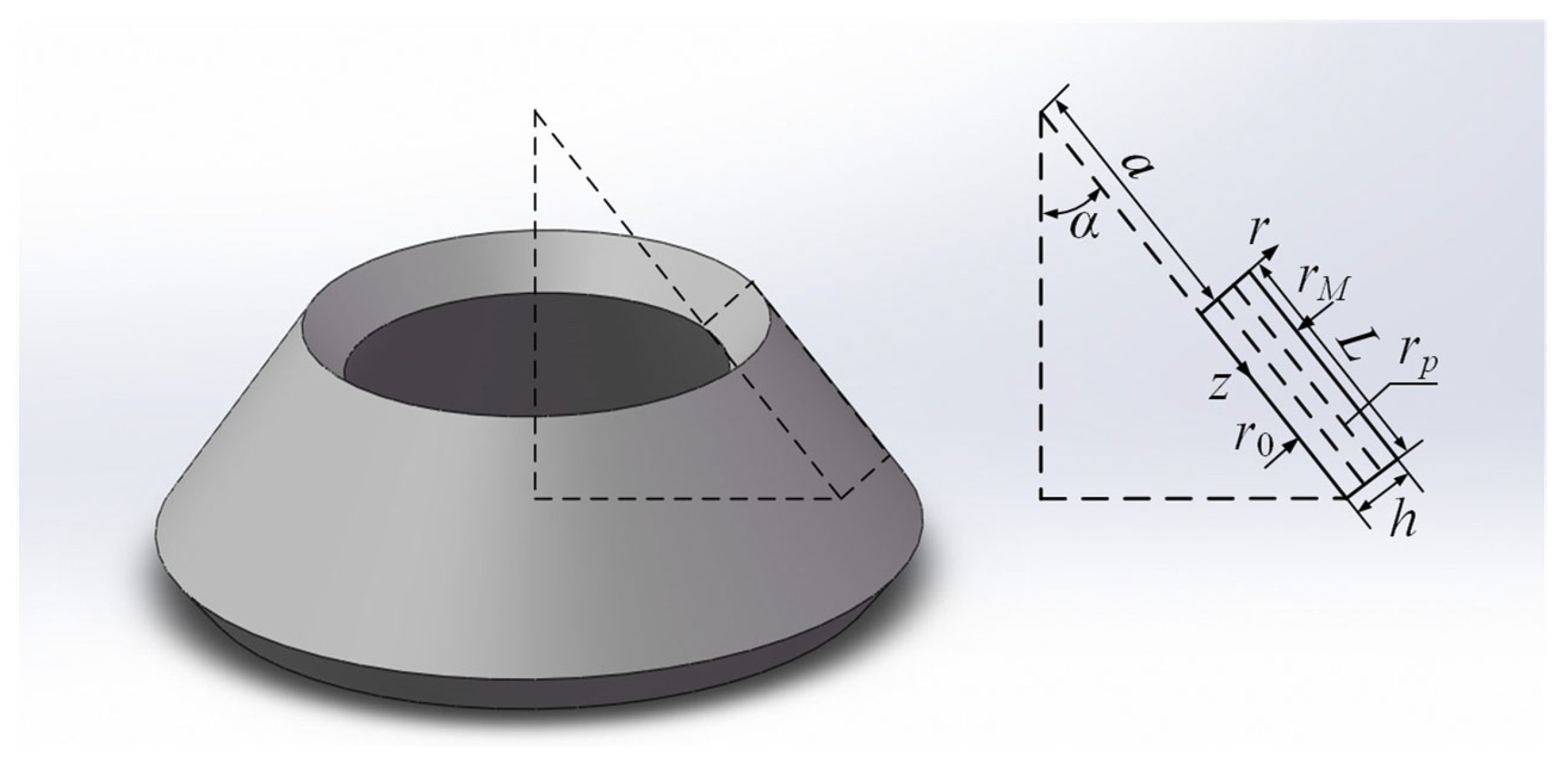
Figure 2.
Normalized displacement mode shapes: (a) comparison of results between SSM and SS-DQM; (b) comparison of results between pseudo-Stroh formalism and SS-DQM.
Figure 2.
Normalized displacement mode shapes: (a) comparison of results between SSM and SS-DQM; (b) comparison of results between pseudo-Stroh formalism and SS-DQM.
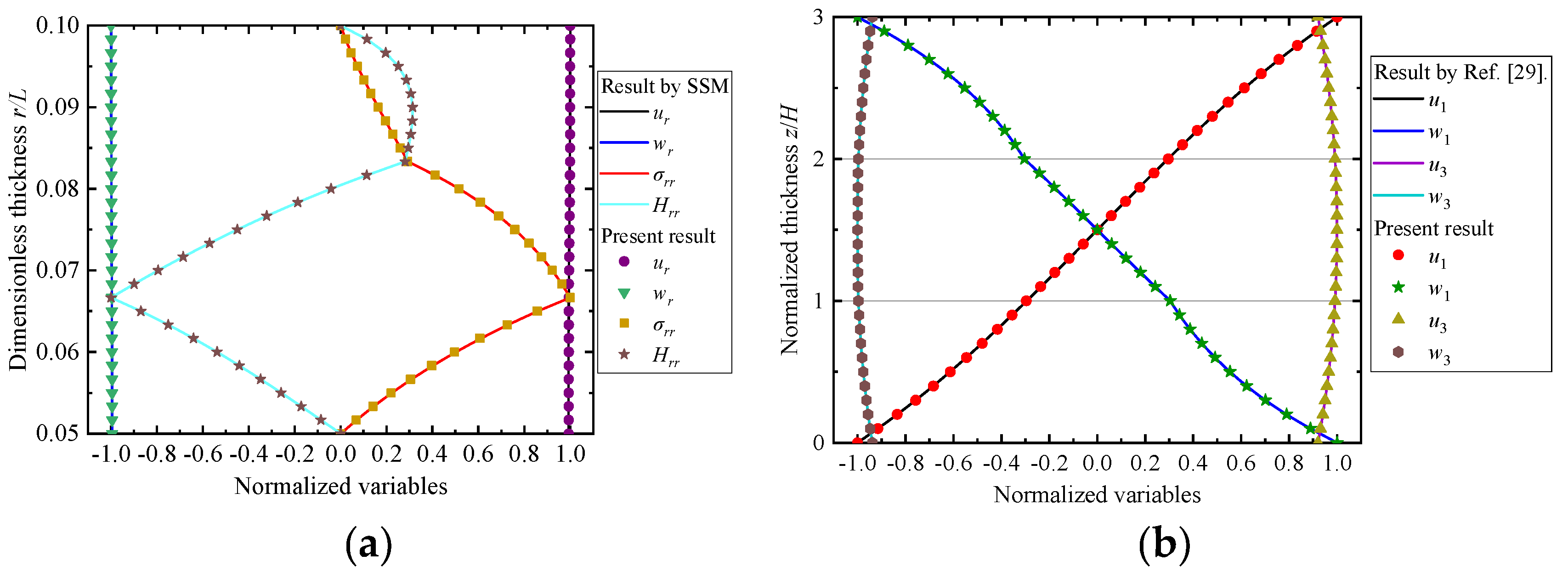
Figure 3.
First-order dimensionless displacement mode shapes: (a) , (b) , (c) , and (d) .
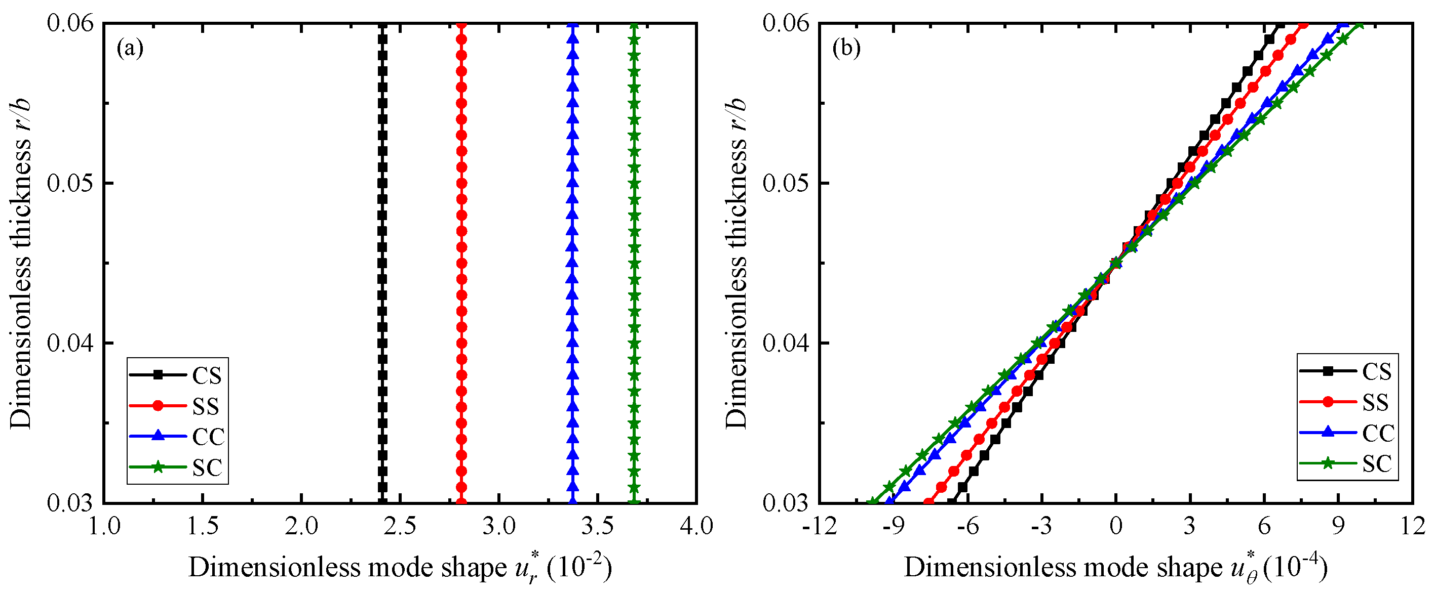
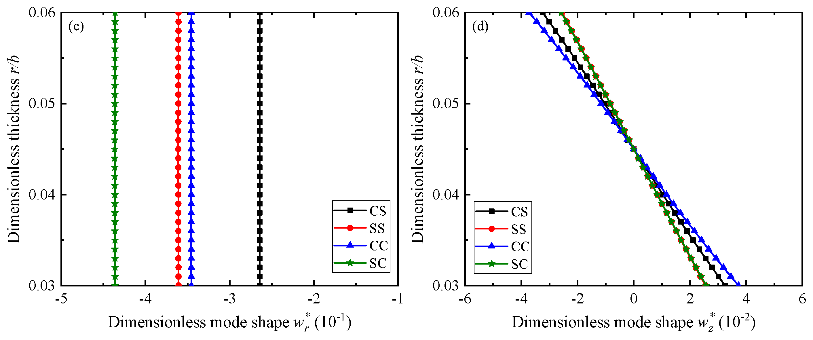
Figure 4.
First-order dimensionless stress mode shapes: (a) , (b) , (c) , and (d)
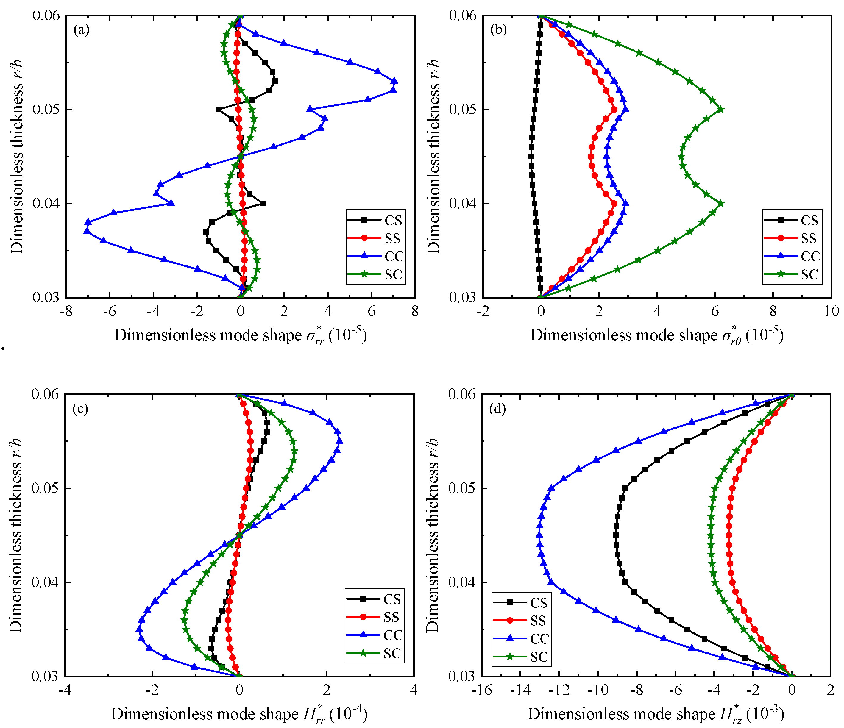
Figure 7.
The contour plots of the phason displacement mode shape (10-3): (a) α0 = π/6, (b) α = π/6, (c) α = π/4, and (d) α = π/3.
Figure 7.
The contour plots of the phason displacement mode shape (10-3): (a) α0 = π/6, (b) α = π/6, (c) α = π/4, and (d) α = π/3.
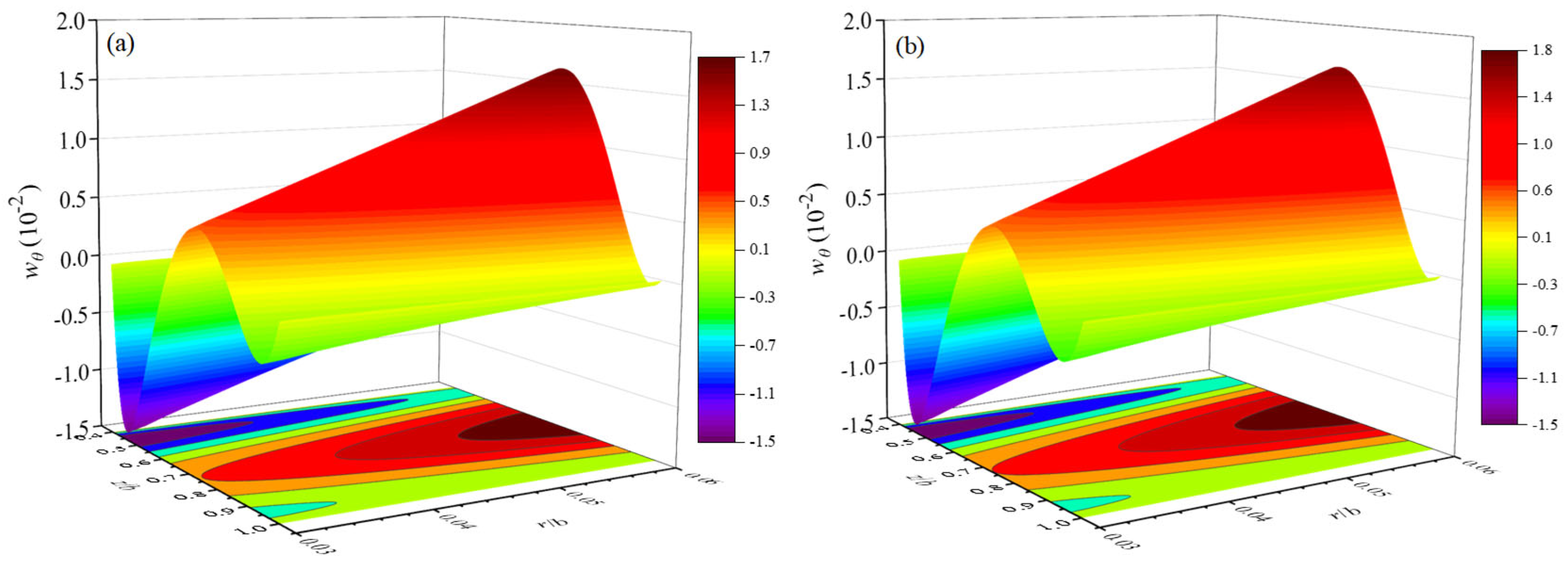
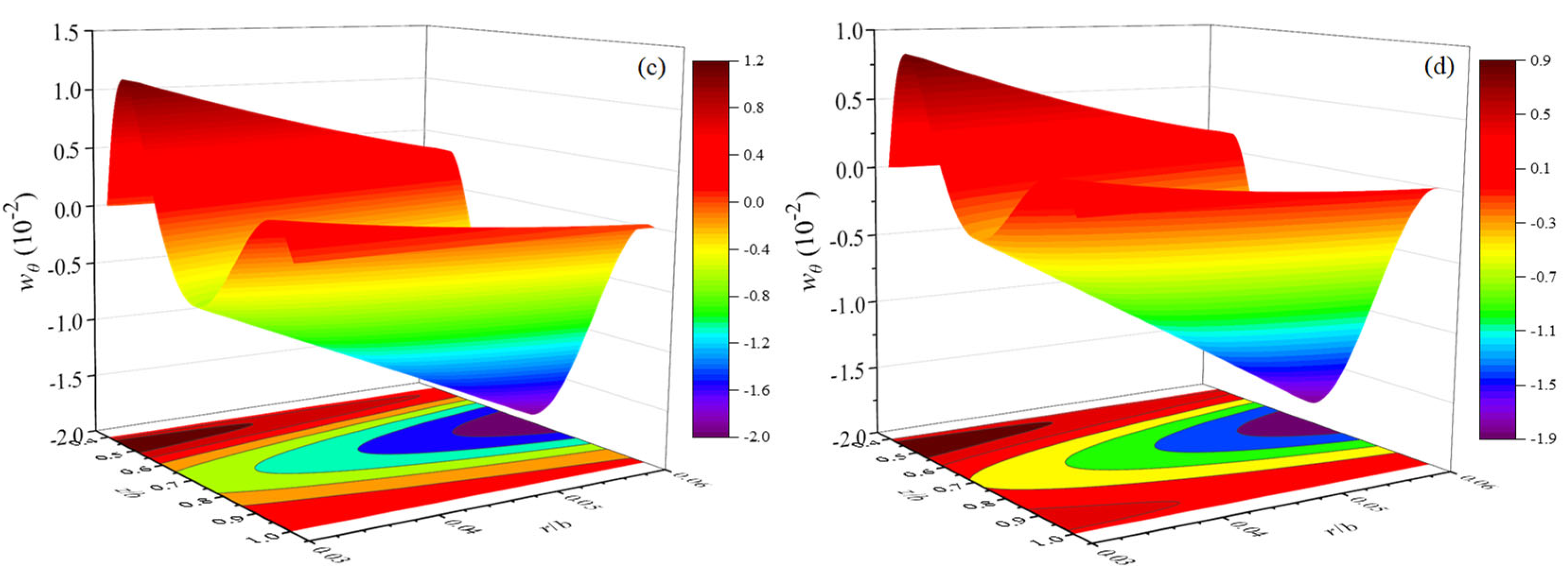
Figure 8.
The contour plots of the phason displacement mode shape (10-3): (a) α0 = π/6, (b) α = π/6, (c) α = π/4, and (d) α = π/3.
Figure 8.
The contour plots of the phason displacement mode shape (10-3): (a) α0 = π/6, (b) α = π/6, (c) α = π/4, and (d) α = π/3.
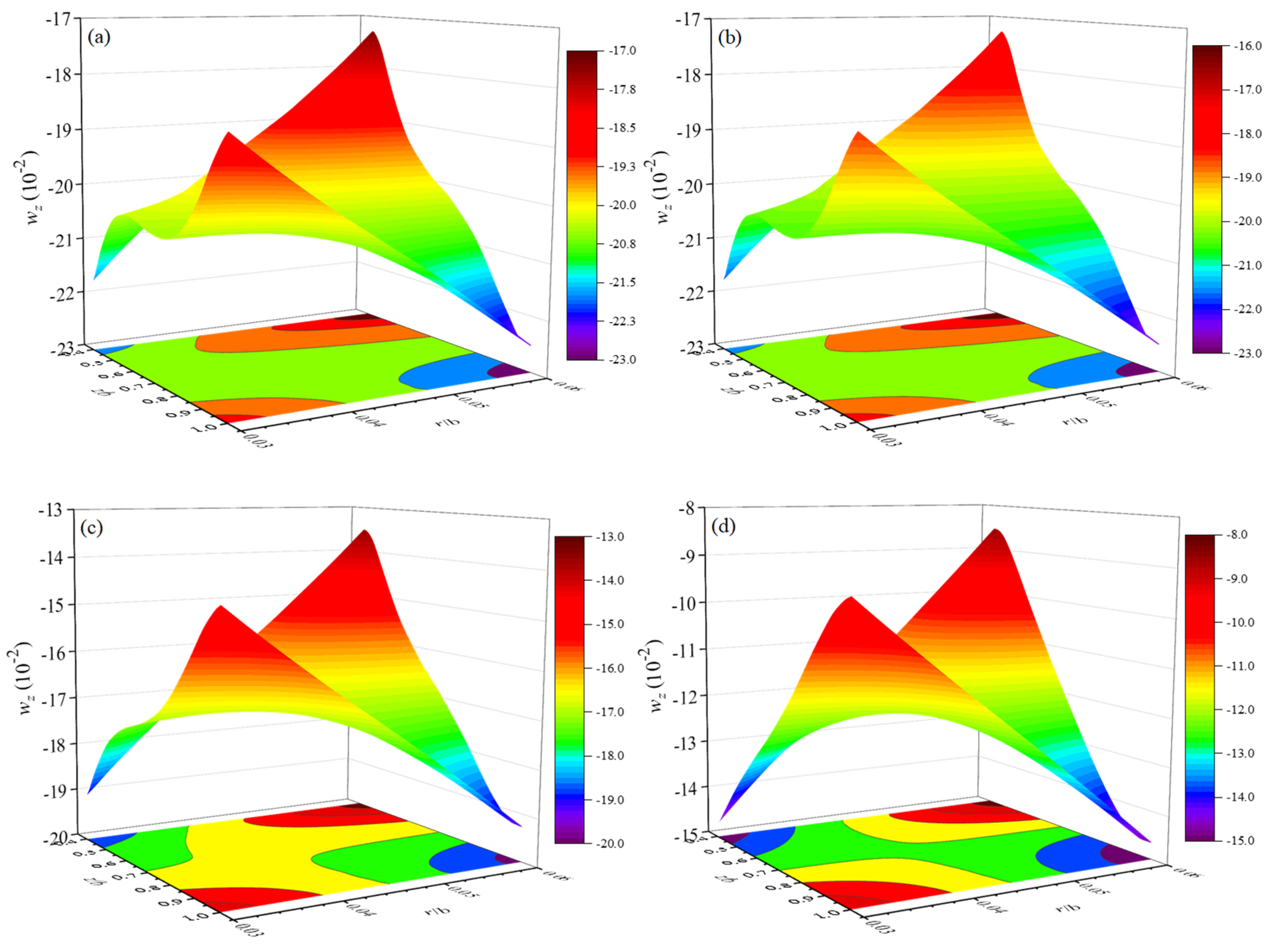
Figure 9.
First-order dimensionless displacement mode shapes: (a) , (b) , (c) , and (d)
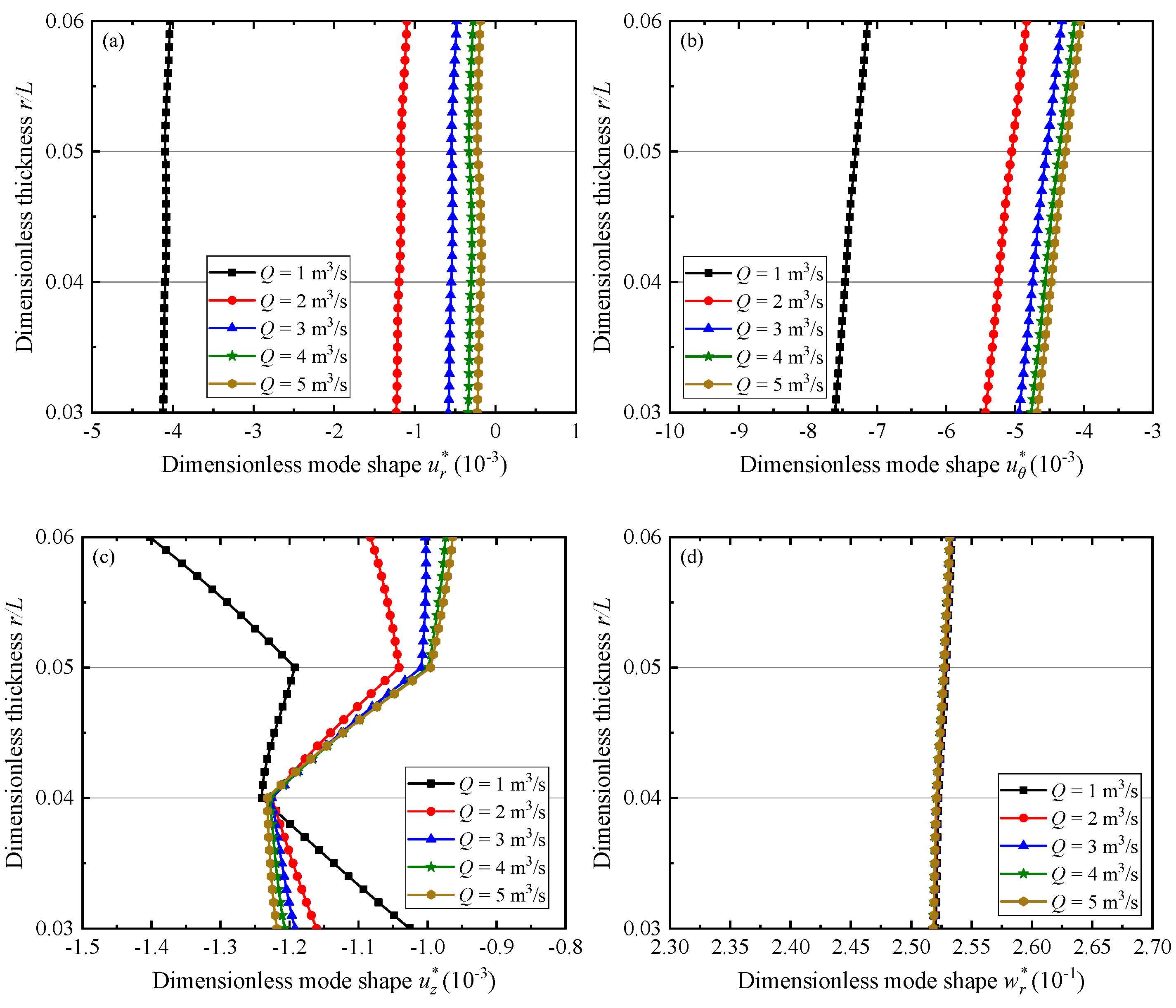
Figure 10.
First-order dimensionless stress mode shapes: (a) , (b) , (c) , and (d)
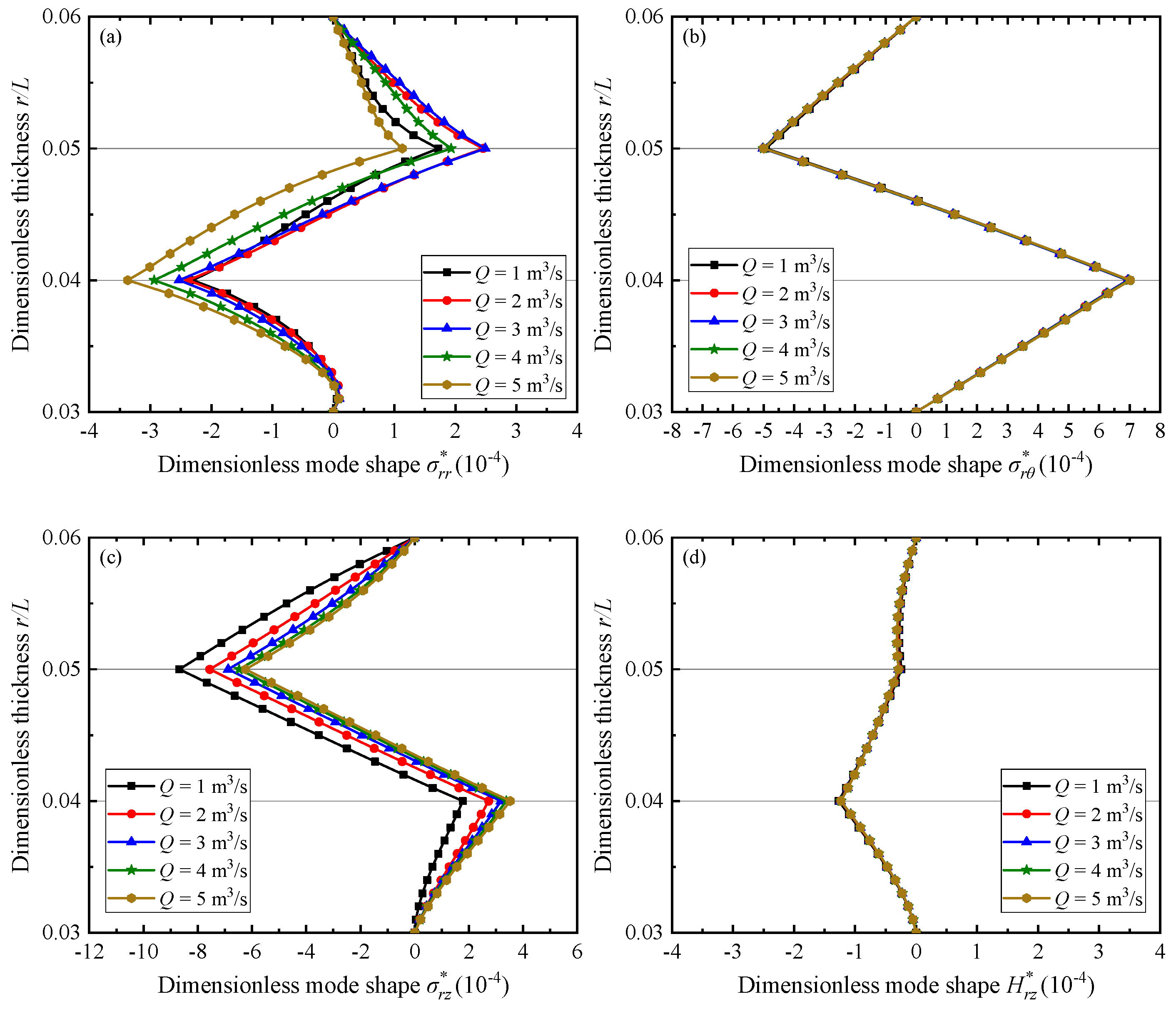

Table 1.
Material properties (C, K, and R in 109 N/m2 and ρ in Kg/m3).
| C11 | C12 | C44 | K11 | K12 | K44 | R1 | R2 | R3 | ρ | |
|---|---|---|---|---|---|---|---|---|---|---|
| QC1 | 234.33 | 57.41 | 70.19 | 122 | 24 | 12 | 8.846 | 4.578 | 3.125 | 4505 |
| QC2 | 112.1 | 60.3 | 32.8 | 60 | 20 | 10 | 5 | -2 | 7 | 5300 |
Table 2.
Comparisons of SS-DQM results for first seven non-dimensional natural frequency Ω with the SSM results for QC cylindrical shells.
Table 2.
Comparisons of SS-DQM results for first seven non-dimensional natural frequency Ω with the SSM results for QC cylindrical shells.
| Mode 1 | Mode 2 | Mode 3 | Mode 4 | Mode 5 | Mode 6 | Mode 7 | |
|---|---|---|---|---|---|---|---|
| Result by SSM | 0.50665 | 0.75775 | 6.26025 | 12.88351 | 18.83285 | 23.90636 | 26.45587 |
| Present result | 0.50665 | 0.75775 | 6.26026 | 12.88351 | 18.83285 | 23.90637 | 26.45588 |
Table 3.
Comparisons of SS-DQM results for first five non-dimensional natural frequency Ω with the exact solutions of the pseudo-Stroh formalism of Ref. [29].
Table 3.
Comparisons of SS-DQM results for first five non-dimensional natural frequency Ω with the exact solutions of the pseudo-Stroh formalism of Ref. [29].
| Mode 1 | Mode 2 | Mode 3 | Mode 4 | Mode 5 | |
|---|---|---|---|---|---|
| Result by Ref. [29] | 1.47999 | 2.38416 | 4.27451 | 8.32909 | 9.52440 |
| Present result | 1.47999 | 2.38417 | 4.27453 | 8.32911 | 9.52443 |
Table 4.
The first nine non-dimensional natural frequency Ω of QC annular plates with different boundary conditions.
Table 4.
The first nine non-dimensional natural frequency Ω of QC annular plates with different boundary conditions.
| Mode 1 | Mode 2 | Mode 3 | Mode 4 | Mode 5 | Mode 6 | Mode 7 | Mode 8 | Mode 9 | |
|---|---|---|---|---|---|---|---|---|---|
| SS | 0.18006 | 0.25376 | 0.66903 | 0.71981 | 0.95204 | 1.16316 | 1.40024 | 1.69379 | 2.05038 |
| CS | 0.25230 | 0.35814 | 0.79363 | 1.15242 | 1.30192 | 1.54856 | 1.96985 | 2.17479 | 2.32465 |
| SC | 0.28126 | 0.39808 | 0.82056 | 1.19096 | 1.52124 | 1.57224 | 2.23517 | 2.36010 | 2.53888 |
| CC | 0.36982 | 0.53056 | 0.94874 | 1.40814 | 1.54224 | 1.71593 | 2.57940 | 2.63754 | 2.78044 |
Table 5.
The first five non-dimensional natural frequency Ω of QC truncated conical shells with different semi-vertical angles.
Table 5.
The first five non-dimensional natural frequency Ω of QC truncated conical shells with different semi-vertical angles.
| Mode 1 | Mode 2 | Mode 3 | Mode 4 | Mode 5 | |
|---|---|---|---|---|---|
| α0 = π/6 | 0.55916 | 0.79145 | 1.13472 | 1.28815 | 1.60288 |
| α = π/6 | 0.55959 | 0.79158 | 1.15277 | 1.28852 | 1.63267 |
| α = π/4 | 0.38664 | 0.71957 | 1.01077 | 1.41469 | 1.60849 |
| α = π/3 | 0.28030 | 0.47297 | 0.82724 | 1.21100 | 1.36207 |
Table 6.
The first nine non-dimensional natural frequency Ω of QC truncated conical shells subjected to flowing fluids.
Table 6.
The first nine non-dimensional natural frequency Ω of QC truncated conical shells subjected to flowing fluids.
| Mode 1 | Mode 2 | Mode 3 | Mode 4 | Mode 5 | Mode 6 | Mode 7 | Mode 8 | Mode 9 | |
|---|---|---|---|---|---|---|---|---|---|
| Q = 1 m3/s | 0.83832 | 1.56236 | 1.75879 | 2.35217 | 2.42893 | 3.26236 | 3.84708 | 4.03837 | 4.17203 |
| Q = 2 m3/s | 0.83946 | 1.56357 | 1.75968 | 2.41162 | 2.43311 | 3.26878 | 3.85937 | 4.18399 | 4.58554 |
| Q = 3 m3/s | 0.83971 | 1.56387 | 1.75992 | 2.42240 | 2.43481 | 3.27066 | 3.85993 | 4.18815 | 4.59383 |
| Q = 4 m3/s | 0.83980 | 1.56399 | 1.76003 | 2.42608 | 2.43588 | 3.27141 | 3.86014 | 4.18988 | 4.59572 |
| Q = 5 m3/s | 0.83985 | 1.56405 | 1.76010 | 2.42784 | 2.43669 | 3.27177 | 3.86026 | 4.19075 | 4.59665 |
Disclaimer/Publisher’s Note: The statements, opinions and data contained in all publications are solely those of the individual author(s) and contributor(s) and not of MDPI and/or the editor(s). MDPI and/or the editor(s) disclaim responsibility for any injury to people or property resulting from any ideas, methods, instructions or products referred to in the content. |
© 2024 by the authors. Licensee MDPI, Basel, Switzerland. This article is an open access article distributed under the terms and conditions of the Creative Commons Attribution (CC BY) license (http://creativecommons.org/licenses/by/4.0/).
Copyright: This open access article is published under a Creative Commons CC BY 4.0 license, which permit the free download, distribution, and reuse, provided that the author and preprint are cited in any reuse.


