Embeddings in Literature Screening: A Gentle Introduction to Vectorial Semantics for Life Science Investigators

As the number of publications is quickly growing in any area of science, the need to efficiently find relevant information amidst a large number of similarly themed articles becomes very important. Semantic searching through text documents has the potential to overcome the limits of keyword-based searches, especially since the introduction of attention-based transformers, which can capture contextual nuances of meaning in single words, sentences or whole documents. The deployment of these computational tools has been made simpler and accessible to investigators in every field of research thanks to a growing number of dedicated libraries, but a knowledge of how meaning representation strategies work is crucial to make the most out of these instruments. The present work aims at introducing the technical evolution of the meaning representation systems, from vectors to embeddings and transformers tailored to life science investigators with no previous knowledge of natural language processing.

Keywords:

embeddings

;

life sciences

;

academic publications

Subject:

Biology and Life Sciences - Life Sciences

1. Introduction: A Needle in a Hastack

The world of academic publishing is undergoing a constant process of acceleration. More research is being conducted by an increasing number of researchers worldwide, more journals are available, publication turnaround is faster. As a result, the number of scientific reports that appear every year online is growing at an exponential rate [1]. With publication numbers exceeding the capabilities of individual scholars to keep up with this unprecedented pace, reviews of any sort, including narrative reviews or systematic reviews, have acquired a growing importance to summarize the state-of-the-art knowledge in any field. To conduct such reviews, however, online data repositories and databases must be queried [2,3], usually with keyword-based approaches, i.e. searching for entries that include one or more desired keywords in their text, usually in their title or abstract [4]. this approach can be very effective – provided that articles use the desired wording - but only partially efficient, because search results are commonly inflated by big numbers of off-topic publications, so that investigators have to spend much time and effort to clean their search results [5].

2. A (Semantic) Space Odyssey

Fortunately, natural language processing (NLP) and machine learning are progressing at a very fast pace and new tools and techniques are being developed that could greatly enhance efficiency and effectiveness in this process. Several such systems are now available on the market, even for literature searches [6]. At the very root of all the algorithms for the analysis of text documents is the ability of these algorithms to create numerical representations of the meaning of texts, through the use of vectors, or, as they are commonly known, embeddings [7].

The concept that a word - or a sentence, or a whole document - can be represented as a vector in a semantic space, based on its co-occurrence with other words within a given lexical context, has origins in the work of Leonard Bloomfield and Zellig Harris that is the basis of Distributional semantics [8,9]. According to this approach, the meaning of a word is defined and can be represented by its context. According to a famous quote by J.R. Firth “You shall know a word by the company it keeps!”.

An example of this could be the somewhat quirky sentence:

“She took a xylinth, and applying a very light pressure, she was able to remove most of the calculus”.

The readers may not be aware what a xylinth is (it is admittedly a made-up word), they may have not heard this word at all, but based on the context, the majority of them would probably convene that this weird word is very likely to denote some kind of tool, maybe a surgical instrument, that can be used in dental practice to remove calculus – maybe from alien teeth.

Distributional semantics undoubtedly possesses an advantage that can be leveraged in NLP, i.e. that all the elements that are necessary to describe the meaning of a word are present in the sentence itself. A meaning representation rooted in distributional semantics does not need to refer to any other knowledge repository, lexicon, or ontology, outside the very sentence that is being represented, and this makes computing leaner and faster.

There are several approaches for constructing semantic vectors from a document or corpus of documents in the field of NLP. One approach to sentence vectors is utilizing co-occurrence matrices that measure the frequency of words appearing together in the text [10]. These vectors are typically long, sparse - i.e. contain a lot of zeros - and – frankly, quite inefficient.

Let’s take two simple sentences, to get a better grasp of the process:

a): Red blood cells transport oxygen.
b): Inflamed tissues are red.

We can build a vocabulary W from these two sentences, using all the occurring words, listing them by lemma (i.e. their dictionary entry):

W= [Red, blood, cell, to transport, oxygen, inflamed, tissue, to be]

We can now turn each sentence into a vector, possibly ignoring those common grammatical words such as articles or prepositions, which are commonly known in NLP as stopwords [11], by assigning the value 1 for each word of W when it is present in the sentence and 0, when it is absent (Table 1).

The first sentence now possesses a vectorial representation [1,1,1,1,1,0,0,0], while the second is [1,0,0,0,0,1,1,1]! Such vectors can be sometimes effective in certain simple NLP tasks but suffer with strong limitations The length of W is given by the size of the vocabulary considered, which can be quite large (in the order of tens or hundreds of thousands, depending on the language and the topic considered). Another important limitation is that the representations of sentences is independent of the order of the words, so that the sentences:

a): Red blood cells transport oxygen
a’): Oxygen transports red blood cells

have identical representations, even though their meaning is different. For this reason, this technique is called “Bag of words” (BoW) [12].

It is easy to guess that very common words, which have little bearing on the meaning of the sentence, can easily receive extra weight in the vectorial representation of a sentence in a document-term matrix. To obviate that, weighing procedures have been developed, such as Tf/Idf, which increases the weight of rarer words [13], while reducing the bearing of more frequent words (to highlight the peculiarities of individual sentences).

Embeddings are dense vectors, and several algorithms exist to compute such embeddings [14]. An example of such an approach is the Word2vec algorithm introduced by Mikolov in 2013, which employs shallow neural networks with just one hidden layer to create word embeddings and has been widely influential in this area [15]. Word2vec relies on the fundamental premise of the distributional hypothesis, assuming that words appearing in similar contexts share similar meanings. The first step is to set a context window, i.e. how many words around a given word we should consider; it could be

\pm

1 word, or more, although there is consensus that the context should not exceed

\pm

3-4 words [16]. Let’s assume we wish to analyze the – probably quite uncontroversial - sentence:

a): Neurology is a difficult but interesting topic

We could eliminate “is”, “a”, “but” (because they are stopwords and do not presumably add much to the semantic content of the embedding), and we would be left with 4 semantically ‘heavier’ lexical elements:

b): Neurology difficult interesting topic

For each word in the sentence, we identify its context; so, assuming a

\pm

1 context window, if we take the word “neurology”, its context is “difficult”; if we consider “difficult” as target word, its context will be “neurology” and “interesting” and so on. We can thus create tuples of (target, context) words:

(neurology, difficult),

(difficult, neurology), (difficult, interesting)

(interesting, difficult), (interesting, topic)

(topic, interesting)

Now that we have tuples of target-context words, Word2Vec offers two primary methods for generating word embeddings: the Continuous Bag of Words (CBOW) and Skip-gram models. In the CBOW model, the objective is to predict a target word based on its context words within a specified window. Conversely, the Skip-gram model flips this process by aiming to predict context words given a target word. Word2vec uses a neural network architecture where the input layer corresponds to the context (or target) words, and the output layer contains its counterpart in the tuple. Training involves adjusting the weights between these layers so that the model gets better at predicting one word given the other. The word embeddings are extracted from the hidden layer's weights, representing words as dense, continuous vectors in a high-dimensional space.

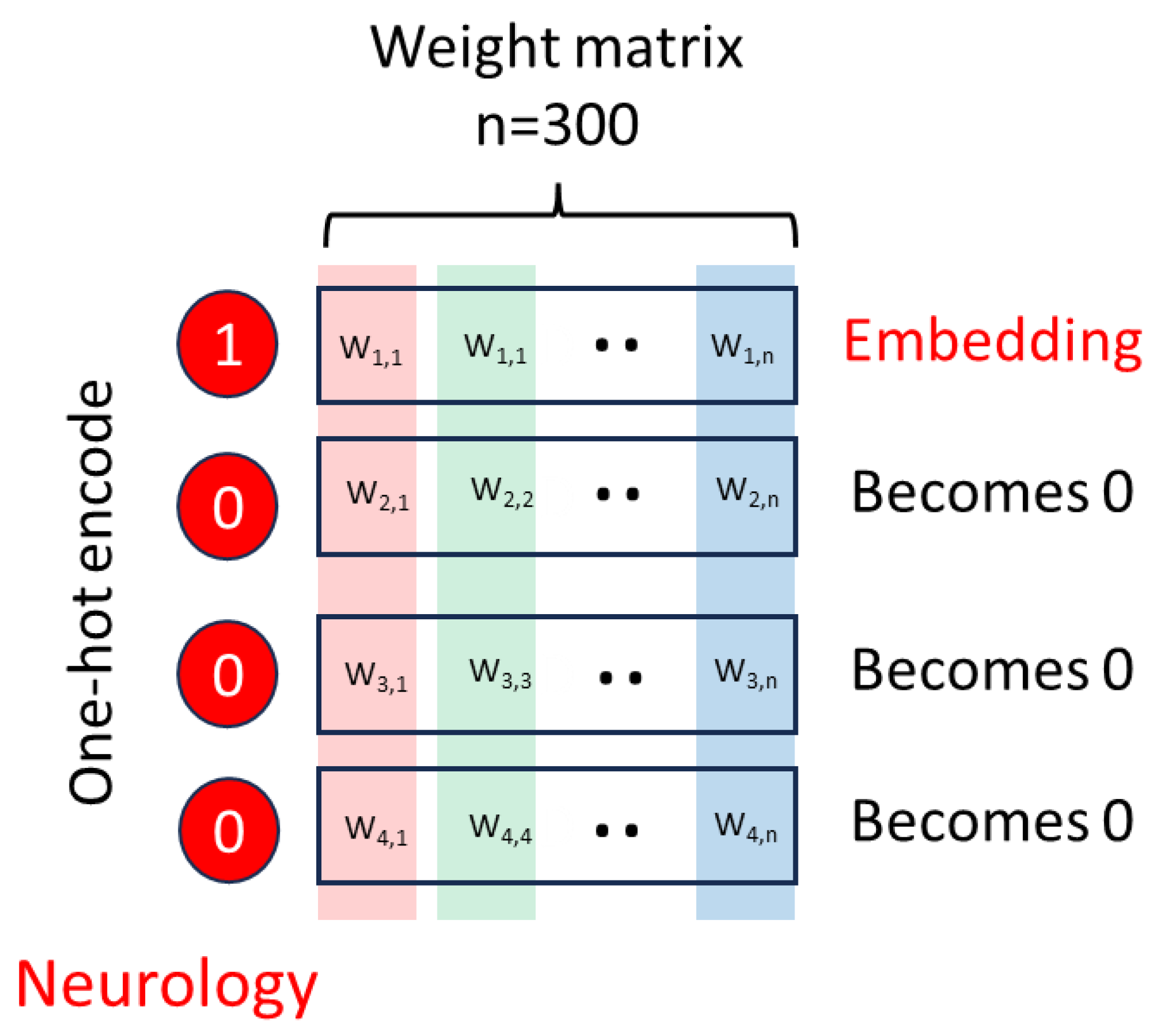
Practically, the algorithm would assign an arbitrary vector to each word (usually relying on the so called “one-hot encode” approach), e.g. as follows:

Neurology = [1,0,0,0]

Difficult = [0,1,0,0]

Interesting = [0,0,1,0]

Topic = [0,0,0,1]

Word2vec would then apply weights (w₁ in Figure 1, for skip-gram architecture) to the input vector that would then get adjusted to maximize the similarity of the output of the neural network to the vector of the target word.

Once trained, Word2Vec generates word embeddings by discarding the original input vectors and taking only the weights associated with each word in the input layer of the neural network (Figure 3). The nature of the learning task makes it so similar weights (and therefore similar embeddings) are assigned to words that can occur interchangeably within similar contexts. For instance, the word cat is closer to the word dog than the word airplane. Moreover, semantic structures tend to be preserved by the embedding, so it is typical to observe relations like

King - Man + Woman ≈ Queen

By using those weights to produce embeddings that encode semantic similarities and relationships among words. Word2Vec's efficiency and ability to capture semantic meaning have made it a cornerstone of natural language processing, enabling a wide range of downstream applications such as text classification, sentiment analysis, and recommendation systems [17,18,19,20].

Once word embeddings are generated, a whole sentence, or even a whole document can be represented, e.g. by joining, or averaging across the embeddings of the words that compose it.

Word2vec suffered with some limitations such as its inability to represent entire documents and its dependency on pre-defined context frames. Word2vec was unable to represent the different meanings a word could have in a context. So, for instance, the word "bank" could refer to a financial institution or the edge of a river, but Word2Vec would assign it a single embedding [21].

Figure 3. Word2Vec creates word embeddings by discarding the input one-hot encode vector and retaining the weights.

3. The Good, the Bad, the Ugly

Word2vec and other similar word embeddings are based on analyzing a small context window. This severely limits their capability to capture the meaning of full sentences, paragraphs, or documents. This limitation is inherited by the Multi-Layer Perceptron (MLP) architecture of the neural network [22]. The connections between neurons in an MLP are, in fact, fixed. Any input will be subjected to exactly the same sequence of operations. Therefore, the input size must be uniform and defined before training.

A more complex architecture, especially designed to deal with variable-length input sequences, is that of Recurrent Neural Networks (RNNs) [23]. In an RNN, the input is a sequence of vectors (e.g., obtained by applying word2vec to the words in a sentence). Each vector is processed by the RNN together with another vector representing a “state” of the computation. The result is an output vector and a new state. The state works as a short-term memory, aggregating information about all the previous input vectors processed so far. In some sense, in RNNs the context window is formed by all vectors preceding the one being processed.

However, the capacity of the state vector is limited, and the memory of basic RNNs is typically very short. To improve that, many complex models have been proposed, such as Long-Short-Term-Memory (LSTM, [24]) and Gated Recurrent Units (GRU, [25]).

RNNs became the de-facto standard for most applications in natural language processing. They are especially suitable for the implementation of autoregressive models, that is, models that anticipate the next word in a sentence, given all the preceding ones [26]

4. Transformers, More than Meets the Eye

In recent years, Transformers have become a significant advancement in the field of literature screening, greatly improving research efficiency. Their introduction can be traced back to the seminal paper "Attention is All You Need" by Vaswani et al. in 2017, and has since paved the way for state-of-the-art NLP models such as BERT, or GPT, among others [27]. Transformers offer an alternative architecture that addresses some limitations of traditional word embedding learning methods by incorporating contextual information for downstream tasks. Specifically designed to handle sequences of data, transformer models are well-suited for NLP tasks requiring a thorough understanding of word context within sentences. This is achieved through the inclusion of self-attention, a mechanism that allows the model to assign varying levels of importance to different segments during processing.

Unlike traditional neural networks, where connections between the neurons are fixed at design time, networks with attention mechanisms may learn to route information adaptively, greatly improving their capabilities. Given a sequence of vectors x_1,x_(2 ),...,x_T (perhaps vectors in a word embedding), self-attention uses three matrices of learnable weights to linearly project them into three T × D matrices of keys (K), values (V), and queries (Q). Then, the following expression is computed:

Y = s o f t m a x (\frac{K Q^{T}}{\sqrt{D}}) V

where the product KQ^T computes a matching score for each combination of a key and a query vector. The softmax operator converts the set of scores for each query into coefficients in the [0, 1] range, and the last product computes convex combinations of the value vectors by using those coefficients. The √D term is just needed to scale the scores in a suitable range. The result is the T × D matrix Y, whose rows y_1,y_(2 ),...,y_T represent a transformed version of the input sequence. Note that all input vectors contribute to all output vectors, but with a weight determined by the matching between keys and queries. Note that self-attention does not inherently consider the position in the sequences. To address this limitation, positional encodings are combined with word embeddings to provide a numerical representation of the relative positions of each token within the sequence.

Briefly, transformers are neural networks that include multiple self-attention layers and many other standard layers [28]. They progressively transform the input by aggregating information across all positions in the sequence. In the case of language models, transformers are trained to predict the next token or to fill artificial gaps in sentences taken from a large corpus of text. After training, the model can be used as is or fine-tuned for a specific downstream task such as sentiment analysis, sentence similarity assessment, natural language inference, question-answering systems, and reading comprehension evaluations.

5. Far Away, so Close

A literature search requires the operator to be able to discriminate among papers [29]. This usually involves the investigator to possess some questions that has be answered. The process of choosing or discarding literature is then usually a process whereby an article retrieved by the search is compared to the query [30]. To put it simply, if they topics are closely related, then it is a match and paper can be saved, otherwise it will be discarded. For an A.I. to work, it is imperative that the algorithm possess a way to measure the relatedness of the document meaning to other documents [31]. Fortunately, once embeddings are created, it is possible to measure their similarity mathematically and get a sense of how similar the meaning of words or sentences is. One such methods is cosine similarity, a widely used concept in NLP that measures the similarity between two non-zero vectors in a multi-dimensional space. Specifically, it quantifies the cosine of the angle between these vectors when they are represented as points in this space. In simpler terms, cosine similarity evaluates how closely aligned the directions of two vectors are, regardless of their magnitudes. This property makes it particularly valuable for comparing documents or text data, where the vectors can represent the frequency of words or other features. To compute cosine similarity, the cosine of the angle between two vectors is calculated as the dot product of the vectors divided by the product of their magnitudes [32].

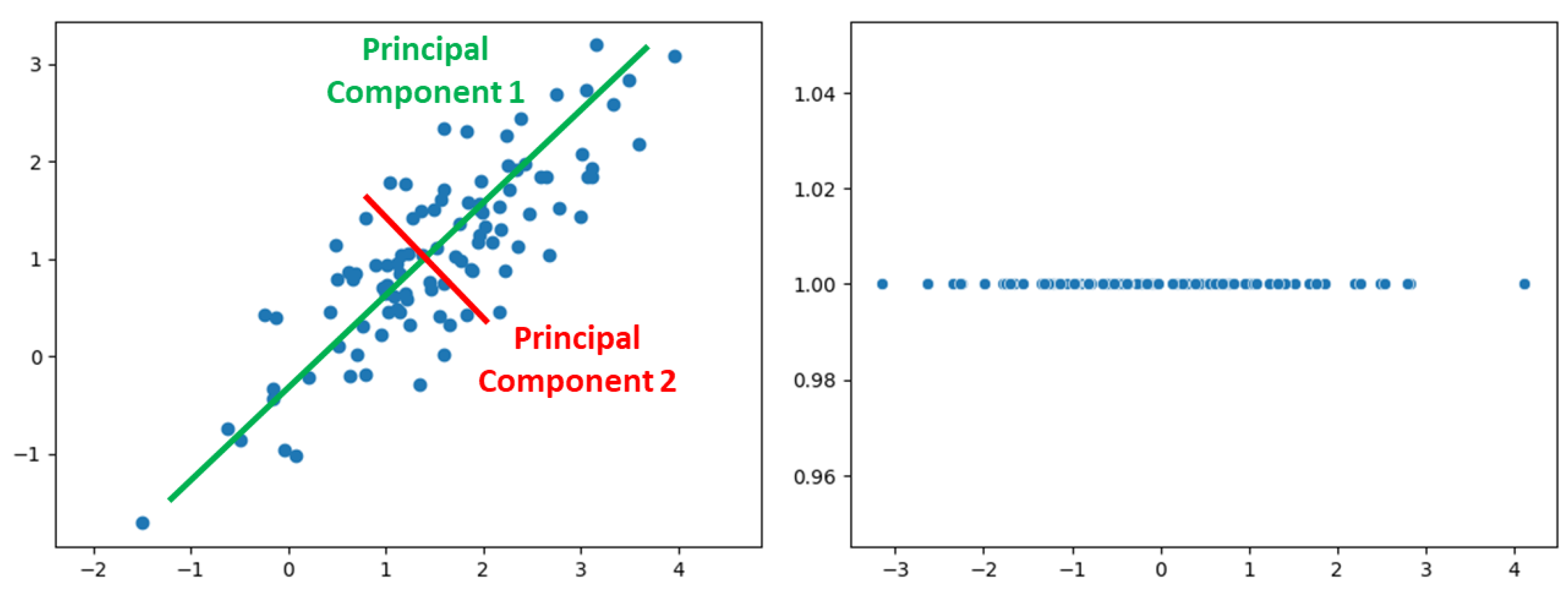
Figure 4. Principal Component Analysis is one algorithm for dimensionality reduction, which works by picking the components (i.e. the dimensions) along which the data show the greatest degree of variation.

The resulting similarity score ranges from -1 to 1, with 1 indicating perfect similarity (when the vectors are in the same direction), 0 indicating no similarity (when they are orthogonal), and -1 indicating perfect dissimilarity (when they are in opposite directions). Cosine similarity offers advantages over other similarity metrics, such as the Jaccard similarity [33], because it takes into account not only the presence or absence of elements but also their relative frequencies. Moreover, cosine similarity is computationally efficient and can handle high-dimensional data effectively.

Similarity between embeddings can also be represented graphically, though there is a notable obstacle to that: we cannot plot graphs in more than 3 dimensions, due to the physical constraints of the reality we live in, and vectors can have hundreds, and thousands of dimensions. Fortunately, there are mathematical methods to reduce the number of dimensions of a vector, preserving as much information as possible. One common approach to dimensionality reduction is Principal Component Analysis (PCA), whose mathematical basis was defined at the beginning of the 20^th century [34] and which identifies orthogonal axes (principal components) along which the data varies the most. By projecting the data onto a subset of these principal components, PCA reduces dimensionality while minimizing information loss (Figure 4) [35].

Another widely used technique is t-Distributed Stochastic Neighbor Embedding (t-SNE), which focuses on preserving the pairwise similarity structure between data points, making it particularly useful for visualization and clustering tasks [36]. Linear Discriminant Analysis (LDA) is another method that seeks to maximize class separability in supervised learning settings, making it valuable for classification problems [53]. Non-linear dimensionality reduction techniques, such as Isomap and Locally Linear Embedding (LLE), address scenarios where data relationships are more complex and cannot be captured by linear transformations [54]. Isomap constructs a low-dimensional representation by estimating the geodesic distances between data points on a manifold, preserving the intrinsic geometry of the data. LLE, on the other hand, seeks to retain local relationships between data points, making it suitable for preserving the fine-grained structure of the data. More recently, UMAP (Uniform Manifold Approximation and Projection) has been introduced, with the purpose of preserving the topological structure of the high-dimensional graph at lower dimensions, by constructing a high-dimensional graph representation of the data, where each data point is connected to its nearest neighbors and then creating a lower-dimensional graph that best approximates this structure [55].

As an example, we can take a set of 10 titles from the literature:

Porous titanium granules in the treatment of peri-implant osseous defects-a 7-year follow-up study, reconstruction of peri-implant osseous defects: a multicenter randomized trial [56],
Porous titanium granules in the surgical treatment of peri-implant osseous defects: a randomized clinical trial [57],
D-plex500: a local biodegradable prolonged release doxycycline-formulated bone graft for the treatment for peri-implantitis. a randomized controlled clinical study [58],
Surgical treatment of peri-implantitis with or without a deproteinized bovine bone mineral and a native bilayer collagen membrane: a randomized clinical trial [59],
Effectiveness of enamel matrix derivative on the clinical and microbiological outcomes following surgical regenerative treatment of peri-implantitis. a randomized controlled trial [60],
Surgical treatment of peri-implantitis using enamel matrix derivative, an rct: 3- and 5-year follow-up [61],
Surgical treatment of peri-implantitis lesions with or without the use of a bone substitute-a randomized clinical trial [62],
Peri-implantitis - reconstructive surgical therapy [63].

and turn them into embeddings using the freely available pre-trained all-MiniLM-L6-v2 transformer model. This model has a transformer-based architecture that can turn any sentence into an embedding.

As an example, (part of) the 384-dimensional embedding for the first title of the list is reported below:

-2.29407530e-02, 1.49187818e-03, 9.16108266e-02, 1.75204929e-02, -8.36422145e-02, -6.10548146e-02, 8.30101445e-02, 3.96910682e-02, 1.58667186e-04, -2.62408387e-02, -7.69069120e-02, 4.60811984e-03, 8.64421800e-02, 7.87990764e-02, -4.33325134e-02, 2.49587372e-02, 2.24952400e-02, -2.90464610e-02, 3.59166898e-02, 4.27976809e-02, 7.94209242e-02, -5.87367006e-02, -6.49892315e-02, -8.70294198e-02, -5.51731326e-02, 4.95349243e-03, -3.01233679e-02, -3.23325321e-02, -1.54273247e-03, 5.24741262e-02, -7.11492598e-02, 5.16711324e-02, -4.42666225e-02, -6.38814121e-02, 6.46011531e-02, -4.63259555e-02, -9.23364013e-02, -3.56980823e-02, -9.30937752e-02, 1.27522862e-02, 5.05894162e-02, 5.07237464e-02, -9.00633708e-02, 6.91129547e-03, 4.79323231e-02, -6.69493945e-03, 1.27279535e-01, -6.33438602e-02, 2.78936550e-02, -3.34392674e-02, -6.21677283e-03, -4.32619415e-02, 5.89787960e-02, -9.10086110e-02, -2.79910862e-02, -5.80033176e-02, -5.82423434e-02, -6.41746866e-03, 4.17577056e-03, -1.90278993e-03, 6.72984421e-02, -4.39932309e-02, …. 1.52898552e-02, 9.40597132e-02, -3.60338315e-02

The only way we can plot such an embedding is by reducing its dimensions to 3 or 2, so that we can use those as cartesian coordinates in a 3D or 2D graph respectively. By applying PCA the very same embedding can be reduced to:

0.5363835, 0.1012947

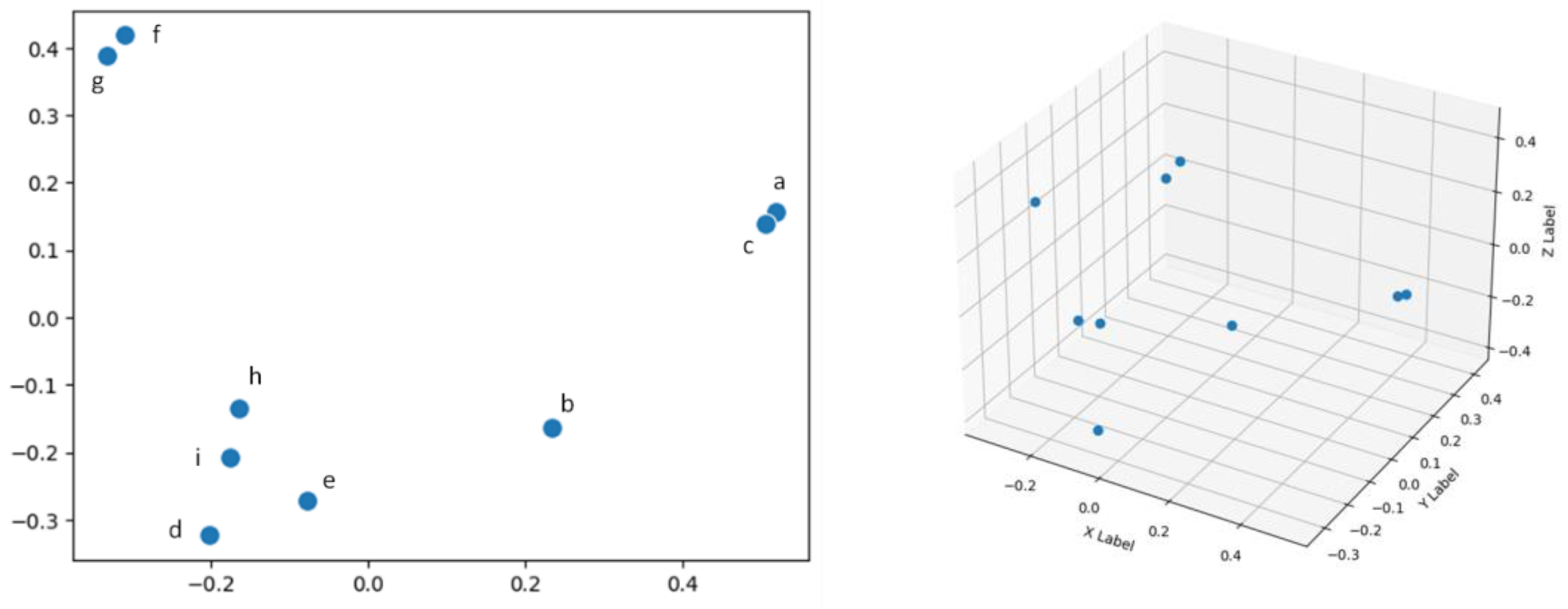
Each title is therefore now represented by only 2 values, which are less effective in describing all the semantic nuances of the title but can be used as cartesian coordinates in an x, y space, i.e. these reduced embeddings can now be plotted as dots within a semantic space in a 2D scatterplot (Figure 5A), where the distance between dots is a visual representation of the semantic distance between titles, or, for an even more detailed representation of the relationship between titles, in a 3D plot (Figure 5B).

Figure 5. Embeddings can be reduced to two or three dimensions and used as Cartesian coordinates within a semantic space. The closer the points in the scatterplot, the closer the semantics of the words.

However, dimensionality reduction is not without challenges and trade-offs [64]. Aggressive reduction can lead to information loss, and choosing the appropriate dimensionality reduction method and the number of dimensions to retain requires careful consideration and experimentation [65]. Moreover, it may not always be suitable for all datasets; its effectiveness depends on the data's inherent structure and the specific task at hand. Nevertheless, when applied with discernment, dimensionality reduction techniques can be invaluable tools for simplifying complex data, improving model performance, and gaining insights from high-dimensional datasets in a wide range of applications [66].

6. Everything Everywhere All at Once

The advent of Large Language Models (LLMs) like the Generative Pre-trained Transformer (GPT) series developed by OpenAI [67] has significantly transformed NLP and its applications [68]. These models are "large" both in terms of the volume of data they are trained on and the complexity of their underlying neural networks [69]. LLMs are distinguished by their capacity to understand, generate, and interpret human language with a degree of proficiency that allows them to perform a wide range of language-based tasks [70]. As these models evolve, becoming larger and more sophisticated, their potential in literature review and information retrieval is growing exponentially [71,72]. The ability to sift through the vast expanses of the internet and extract precise data and information is becoming very real, bolstered by the continuous release of open models and advancements in the underlying technology. Meta's introduction of the Llama series, or Google’s Gemini or PaLM models, highlights the competition among private and public stakeholders in developing LLMs that are both powerful and capable of nuanced understanding [73].

The integration of Retrieval-Augmented Generation techniques with LLMs further enhances their ability to generate informed and contextually relevant content by retrieving information from a broad array of sources on the internet [74]. This approach could radically transform how we retrieve, use, and interact with information online. RAG functions by coupling a retrieval component with a generative model, allowing the system to fetch relevant information from external databases - even just the internet - in real-time, without relying only on the knowledge that the model has acquired during training.

Despite these advancements and the tools that are becoming available [75], the integration of AI in literature search and evidence collection still necessitates human interaction. This synergy between human oversight and AI's computational power ensures that the outputs are not only relevant but also accurate. The goal, however, remains to achieve a level of sophistication where AI can autonomously conduct literature reviews with minimal to no human intervention, a milestone that seems increasingly attainable as the technology progresses.

The practical applications of such models are already being realized and implemented at unprecedented pace. As we look to the future, the trajectory of LLMs suggests a continued enhancement in their ability to process and understand language at a level of depth and subtlety previously unattainable. The integration of these models into information retrieval and research processes promises to revolutionize how we navigate and utilize the wealth of knowledge available online, moving us closer to a world where AI can autonomously manage complex tasks of data and information retrieval with high sensitivity and sensibility.

Author Contributions

Conceptualization, C.G.; methodology, C.C.; investigation, N.D.; data curation, C.C.; writing—original draft preparation, C.G. and E.C.; writing—review and editing, S.G; supervision, N.D. All authors have read and agreed to the published version of the manuscript.

Funding

This research received no external funding.

Institutional Review Board Statement

Not applicable.

Data Availability Statement

Data are available upon request.

Conflicts of Interest

The authors declare no conflicts of interest.

References

Landhuis, E. Scientific Literature: Information Overload. Nature 2016, 535, 457–458. [Google Scholar] [CrossRef] [PubMed]
Dickersin, K.; Scherer, R.; Lefebvre, C. Systematic Reviews: Identifying Relevant Studies for Systematic Reviews. Bmj 1994, 309, 1286–1291. [Google Scholar] [CrossRef]
Bramer, W.M.; Rethlefsen, M.L.; Kleijnen, J.; Franco, O.H. Optimal Database Combinations for Literature Searches in Systematic Reviews: A Prospective Exploratory Study. Syst Rev 2017, 6, 1–12. [Google Scholar] [CrossRef] [PubMed]
Lu, Z. PubMed and beyond: A Survey of Web Tools for Searching Biomedical Literature. Database 2011, 2011, baq036–baq036. [Google Scholar] [CrossRef] [PubMed]
Grivell, L. Mining the Bibliome: Searching for a Needle in a Haystack? EMBO Rep 2002, 3, 200–203. [Google Scholar] [CrossRef] [PubMed]
Khalil, H.; Ameen, D.; Zarnegar, A. Tools to Support the Automation of Systematic Reviews: A Scoping Review. J Clin Epidemiol 2022, 144, 22–42. [Google Scholar] [CrossRef]
Jurafsky, D.; Martin, J.H. Vector Semantics and Embeddings. Speech and Language Processing 2019, 1–31. [Google Scholar]
Turney, P.D.; Pantel, P. From Frequency to Meaning: Vector Space Models of Semantics. Journal of Artificial Intelligence Research 2010, 37, 141–188. [Google Scholar] [CrossRef]
Harris, Z.S. Distributional Structure. Word 1954, 10, 146–162. [Google Scholar] [CrossRef]
Erk, K. Vector Space Models of Word Meaning and Phrase Meaning: A Survey. Lang Linguist Compass 2012, 6, 635–653. [Google Scholar] [CrossRef]
Saif, H.; Fernandez, M.; He, Y.; Alani, H. On Stopwords, Filtering and Data Sparsity for Sentiment Analysis of Twitter. 2014. [Google Scholar]
Zhang, Y.; Jin, R.; Zhou, Z.-H. Understanding Bag-of-Words Model: A Statistical Framework. International journal of machine learning and cybernetics 2010, 1, 43–52. [Google Scholar] [CrossRef]
Jing, L.-P.; Huang, H.-K.; Shi, H.-B. Improved Feature Selection Approach TFIDF in Text Mining. In Proceedings of the Proceedings. International Conference on Machine Learning and Cybernetics; IEEE, 2002; Vol. 2, pp. 944–946.
Wang, S.; Zhou, W.; Jiang, C. A Survey of Word Embeddings Based on Deep Learning. Computing 2020, 102, 717–740. [Google Scholar] [CrossRef]
Mikolov, T.; Chen, K.; Corrado, G.; Dean, J. Efficient Estimation of Word Representations in Vector Space. arXiv preprint arXiv:1301.3781 2013. arXiv:1301.3781 2013.
Di Gennaro, G.; Buonanno, A.; Palmieri, F.A.N. Considerations about Learning Word2Vec. J Supercomput 2021, 1–16. [Google Scholar] [CrossRef]
Al-Saqqa, S.; Awajan, A. The Use of Word2vec Model in Sentiment Analysis: A Survey. In Proceedings of the Proceedings of the 2019 international conference on artificial intelligence, robotics and control; 2019; pp. 39–43. 201939–43.
Haider, M.M.; Hossin, M.A.; Mahi, H.R.; Arif, H. Automatic Text Summarization Using Gensim Word2vec and K-Means Clustering Algorithm. In Proceedings of the 2020 IEEE Region 10 Symposium (TENSYMP); IEEE, 2020; pp. 283–286.
Ibrohim, M.O.; Setiadi, M.A.; Budi, I. Identification of Hate Speech and Abusive Language on Indonesian Twitter Using the Word2vec, Part of Speech and Emoji Features. In Proceedings of the Proceedings of the 1st International Conference on Advanced Information Science and System; 2019; pp. 1–5.
Jatnika, D.; Bijaksana, M.A.; Suryani, A.A. Word2vec Model Analysis for Semantic Similarities in English Words. Procedia Comput Sci 2019, 157, 160–167. [Google Scholar] [CrossRef]
Liu, Q.; Kusner, M.J.; Blunsom, P. A Survey on Contextual Embeddings. arXiv preprint arXiv:2003.07278 2020.
Kruse, R.; Mostaghim, S.; Borgelt, C.; Braune, C.; Steinbrecher, M. Multi-Layer Perceptrons. In Computational intelligence: a methodological introduction; Springer, 2022; pp. 53–124.
Salehinejad, H.; Sankar, S.; Barfett, J.; Colak, E.; Valaee, S. Recent Advances in Recurrent Neural Networks. arXiv preprint arXiv:1801.01078 2017.
Hochreiter, S.; Schmidhuber, J. Long Short-Term Memory. Neural Comput 1997, 9, 1735–1780. [Google Scholar] [CrossRef] [PubMed]
Cho, K.; Van Merriënboer, B.; Gulcehre, C.; Bahdanau, D.; Bougares, F.; Schwenk, H.; Bengio, Y. Learning Phrase Representations Using RNN Encoder-Decoder for Statistical Machine Translation. arXiv preprint arXiv:1406.1078 2014.
Yin, W.; Kann, K.; Yu, M.; Schütze, H. Comparative Study of CNN and RNN for Natural Language Processing. arXiv preprint arXiv:1702.01923 2017.
Vaswani, A.; Shazeer, N.; Parmar, N.; Uszkoreit, J.; Jones, L.; Gomez, A.N.; Kaiser, Ł.; Polosukhin, I. Attention Is All You Need. Adv Neural Inf Process Syst 2017, 30. [Google Scholar]
Wolf, T.; Debut, L.; Sanh, V.; Chaumond, J.; Delangue, C.; Moi, A.; Cistac, P.; Rault, T.; Louf, R.; Funtowicz, M.; et al. Transformers: State-of-the-Art Natural Language Processing. In Proceedings of the Proceedings of the 2020 Conference on Empirical Methods in Natural Language Processing: System Demonstrations; Association for Computational Linguistics: Stroudsburg, PA, USA, 2020; pp. 38–45.
Bramer, W.M.; Rethlefsen, M.L.; Kleijnen, J.; Franco, O.H. Optimal Database Combinations for Literature Searches in Systematic Reviews: A Prospective Exploratory Study. Syst Rev 2017, 6, 1–12. [Google Scholar] [CrossRef]
Patrick, L.J.; Munro, S. The Literature Review: Demystifying the Literature Search. Diabetes Educ 2004, 30, 30–38. [Google Scholar] [CrossRef]
Farouk, M. Measuring Text Similarity Based on Structure and Word Embedding. Cogn Syst Res 2020, 63, 1–10. [Google Scholar] [CrossRef]
Li, B.; Han, L. Distance Weighted Cosine Similarity Measure for Text Classification. In; 2013; pp. 611–618.
Ivchenko, G.I.; Honov, S.A. On the Jaccard Similarity Test. Journal of Mathematical Sciences 1998, 88, 789–794. [Google Scholar] [CrossRef]
Pearson, K. LIII. On Lines and Planes of Closest Fit to Systems of Points in Space. The London, Edinburgh, and Dublin philosophical magazine and journal of science 1901, 2, 559–572.
Labrín, C.; Urdinez, F. In R for political data science; Chapman and Hall/CRC, 2020; pp. 375–393.
Van der Maaten, L.; Hinton, G. Visualizing Data Using T-SNE. Journal of machine learning research 2008, 9. [Google Scholar]
Xanthopoulos, P.; Pardalos, P.M.; Trafalis, T.B.; Xanthopoulos, P.; Pardalos, P.M.; Trafalis, T.B. Linear Discriminant Analysis. Robust data mining 2013, 27–33. [Google Scholar]
Friedrich, T. Nonlinear Dimensionality Reduction with Locally Linear Embedding and Isomap. University of Sheffield 2002.
McInnes, L.; Healy, J.; Melville, J. Umap: Uniform Manifold Approximation and Projection for Dimension Reduction. arXiv preprint arXiv:1802.03426 2018.
Andersen, H.; Aass, A.M.; Wohlfahrt, J.C. Porous Titanium Granules in the Treatment of Peri-Implant Osseous Defects—a 7-Year Follow-up Study. Int J Implant Dent 2017, 3, 1–7. [Google Scholar] [CrossRef] [PubMed]
Wohlfahrt, J.C.; Lyngstadaas, S.P.; Rønold, H.J.; Saxegaard, E.; Ellingsen, J.E.; Karlsson, S.; Aass, A.M. Porous Titanium Granules in the Surgical Treatment of Peri-Implant Osseous Defects: A Randomized Clinical Trial. International Journal of Oral & Maxillofacial Implants 2012, 27. [Google Scholar]
Emanuel, N.; Machtei, E.E.; Reichart, M.; Shapira, L. D-PLEX. Quintessence Int (Berl) 2020, 51, 546–553. [Google Scholar]
Renvert, S.; Giovannoli, J.; Roos-Jansåker, A.; Rinke, S. Surgical Treatment of Peri-implantitis with or without a Deproteinized Bovine Bone Mineral and a Native Bilayer Collagen Membrane: A Randomized Clinical Trial. J Clin Periodontol 2021, 48, 1312–1321. [Google Scholar] [CrossRef]
Isehed, C.; Holmlund, A.; Renvert, S.; Svenson, B.; Johansson, I.; Lundberg, P. Effectiveness of Enamel Matrix Derivative on the Clinical and Microbiological Outcomes Following Surgical Regenerative Treatment of Peri-implantitis. A Randomized Controlled Trial. J Clin Periodontol 2016, 43, 863–873. [Google Scholar] [CrossRef] [PubMed]
Isehed, C.; Svenson, B.; Lundberg, P.; Holmlund, A. Surgical Treatment of Peri-implantitis Using Enamel Matrix Derivative, an RCT: 3-and 5-year Follow-up. J Clin Periodontol 2018, 45, 744–753. [Google Scholar] [CrossRef]
Renvert, S.; Roos-Jansåker, A.; Persson, G.R. Surgical Treatment of Peri-implantitis Lesions with or without the Use of a Bone Substitute—a Randomized Clinical Trial. J Clin Periodontol 2018, 45, 1266–1274. [Google Scholar] [CrossRef]
Nct Peri-Implantitis - Reconstructive Surgical Therapy. Available online: https://clinicaltrials.gov/show/NCT03077061 2017 (accessed on 10 April 2022).
Ahmad, N.; Nassif, A.B. Dimensionality Reduction: Challenges and Solutions. In Proceedings of the ITM Web of Conferences; EDP Sciences, 2022; Vol. 43, p. 01017.
Sumithra, V.; Surendran, S. A Review of Various Linear and Non Linear Dimensionality Reduction Techniques. Int. J. Comput. Sci. Inf. Technol 2015, 6, 2354–2360. [Google Scholar]
Zebari, R.; Abdulazeez, A.; Zeebaree, D.; Zebari, D.; Saeed, J. A Comprehensive Review of Dimensionality Reduction Techniques for Feature Selection and Feature Extraction. Journal of Applied Science and Technology Trends 2020, 1, 56–70. [Google Scholar] [CrossRef]
Liu, X.; Zheng, Y.; Du, Z.; Ding, M.; Qian, Y.; Yang, Z.; Tang, J. GPT Understands, Too. AI Open 2023. [Google Scholar] [CrossRef]
Thirunavukarasu, A.J.; Ting, D.S.J.; Elangovan, K.; Gutierrez, L.; Tan, T.F.; Ting, D.S.W. Large Language Models in Medicine. Nat Med 2023, 29, 1930–1940. [Google Scholar] [CrossRef]
Kaddour, J.; Harris, J.; Mozes, M.; Bradley, H.; Raileanu, R.; McHardy, R. Challenges and Applications of Large Language Models. arXiv preprint arXiv:2307.10169 2023.
Wei, J.; Tay, Y.; Bommasani, R.; Raffel, C.; Zoph, B.; Borgeaud, S.; Yogatama, D.; Bosma, M.; Zhou, D.; Metzler, D. Emergent Abilities of Large Language Models. arXiv preprint arXiv:2206.07682 2022.
Hersh, W.R. Search Still Matters: Information Retrieval in the Era of Generative AI. arXiv preprint arXiv:2311.18550 2023.
Zhu, Y.; Yuan, H.; Wang, S.; Liu, J.; Liu, W.; Deng, C.; Dou, Z.; Wen, J.-R. Large Language Models for Information Retrieval: A Survey. arXiv preprint arXiv:2308.07107 2023.
Hadi, M.U.; Qureshi, R.; Shah, A.; Irfan, M.; Zafar, A.; Shaikh, M.B.; Akhtar, N.; Wu, J.; Mirjalili, S. A Survey on Large Language Models: Applications, Challenges, Limitations, and Practical Usage. Authorea Preprints 2023. [Google Scholar]
Lozano, A.; Fleming, S.L.; Chiang, C.-C.; Shah, N. Clinfo. Ai: An Open-Source Retrieval-Augmented Large Language Model System for Answering Medical Questions Using Scientific Literature. In Proceedings of the PACIFIC SYMPOSIUM ON BIOCOMPUTING 2024; World Scientific, 2023; pp. 8–23.
Agarwal, S.; Laradji, I.H.; Charlin, L.; Pal, C. LitLLM: A Toolkit for Scientific Literature Review. arXiv preprint arXiv:2402.01788 2024.

Figure 1. Diagram representing the architecture of Word2Vec shallow neural network.

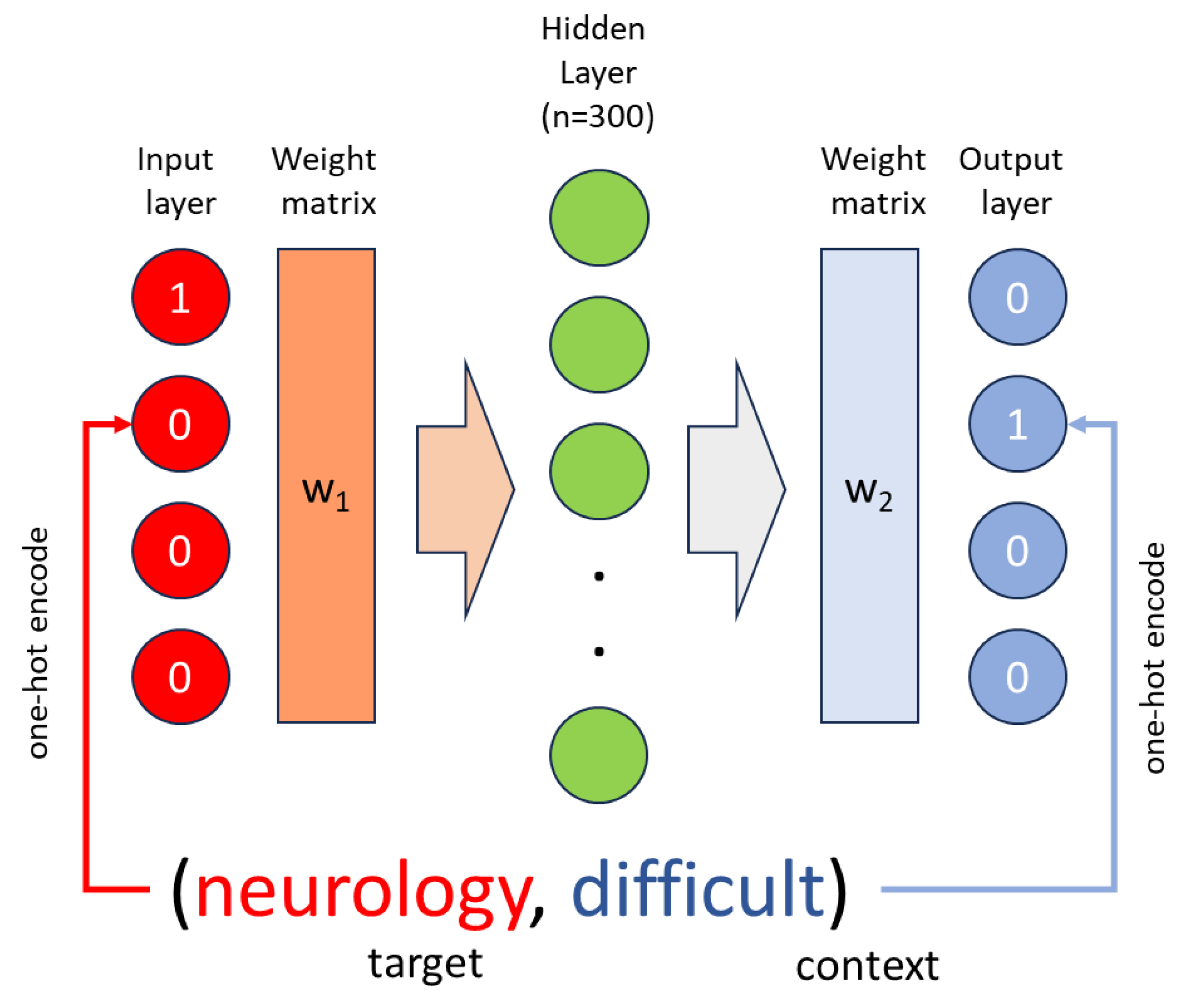
Table 1. Creation of a sentence-term matrix, through the use of a dictionary.

W	Red	Blood	Cell	To transport	Oxygen	Inflamed	Tissue	To be
Sent. A)	1	1	1	1	1	0	0	0
Sent. B)	1	0	0	0	0	1	1	1

Disclaimer/Publisher’s Note: The statements, opinions and data contained in all publications are solely those of the individual author(s) and contributor(s) and not of MDPI and/or the editor(s). MDPI and/or the editor(s) disclaim responsibility for any injury to people or property resulting from any ideas, methods, instructions or products referred to in the content.

© 2024 by the authors. Licensee MDPI, Basel, Switzerland. This article is an open access article distributed under the terms and conditions of the Creative Commons Attribution (CC BY) license (http://creativecommons.org/licenses/by/4.0/).

Copyright: This open access article is published under a Creative Commons CC BY 4.0 license, which permit the free download, distribution, and reuse, provided that the author and preprint are cited in any reuse.

Downloads

Views

Comments

Subscription

Notify me about updates to this article or when a peer-reviewed version is published.

MDPI Initiatives

Important Links

Choose an area of interest and we will send you notifications of new preprints at your preferred frequency.

Disclaimer