
Submitted:
23 August 2024
Posted:
19 September 2024
You are already at the latest version
Abstract
In this study, a computational method is proposed that employs Recurrent Convolutional 1 Neural Networks, utilizing meteorological radar images to forecast storm movement and intensity up 2 to 3 hours ahead, a process known as nowcasting. For this purpose, images from a radar situated in 3 southern Brazil were used. These data are publicly accessible on the website of the National Institute 4 for Space Research (INPE) in Brazil. The approach involves evaluating a spatiotemporal learning 5 recurrent convolutional neural network called PredRNN++. The results were validated through 6 case studies of storms within the radar’s coverage area. To evaluate the performance of the neural 7 network, both visual assessments and metrics such as RMSE and SSIM were employed. The findings 8 indicate that PredRNN++ was effective in simulating the shape and location of the meteorological 9 system.
Keywords:
Neural Network
; Nowcasting
; Radar
1. Introduction
Extreme weather events are particularly important, because they are associated with material and human losses. The weather foerecasting has good skill on relatively slow timescales, because the atmosphere is influenced by high-energy ocean, land, and ice processes that often act on relatively slow timescales [1]. However, severe convective weather forecasting (flash floods, hail, tornadoes, microbursts, and other damaging thunderstorm winds) has poor skill duo the dificult of numerical models represent the physical phenomena in this spatiotemporal scale (nowcasting scale - forecasting limited for periods less than a 3 hours). Duo the difficult of numerical weather forecasting in nowcasting scale, methods based on statistical extrapolation, such as blending thechnique, are explored to deal with this problem [2]. Lately, Machine Learning (ML) techniques have been applied to problems where there is little physical knowledge of the problem [3].
In the [4] the author use an Artificial Neural Networks (ANN) in short-term prediction of Global Solar Irradiance (GSI). The author predict a short-term GSI with error rates less than 20% RMSE. Furthermore, using observations from neighboring stations within a 55 km as a reference radius reduced error rates in predictions for time frames between 1 and 3 h.
Razaque et al. (2017) [5] presents a short-term wind speed forecasting using statistical and ML methods. The authors compare a Generalised Additive Models (GAN-NN) to Stochastic Gradient Boosting (SGB) using data obtained from the South African Wind Atlas Project. The results of the comparative analysis suggest that ANN displays superior predictive performance based on Root Mean Square Error (RMSE). In contrast, SGB shows outperformance in terms of Mean Average Error (MAE).
In [6] authors propose a novel approach, RainPredRNN, which is the combination of the UNet segmentation model and the PredRNN-v2 deep learning model for precipitation nowcasting with weather radar echo images. The proposed model has produced improved performance, about 0.43, 0.95, and 0.94 of MAE, Similarity Index Measure (SSIM), and Critical Success Index (CSI), respectively, with only 30% of training time compared to the other methods.
In this reserach is propose a model based on Recurrent Convolutional Neural Networks (RNCR) for short-term weather forecasting (Nowcasting). This approach is an alternative to traditional statistical extrapolation techniques. The RNCR known as PredRNN++ is a supervised network. Are used as RNCR input/output, images from four meteorological radars located in southern Brazil, available for free access on the website at National Institute for Space Research (INPE). In order to verify the PredRNN++ accuracy is applied RMSE e SSIM and also empirical analyses in tornado that occurred in southern Brazil on June 12, 2018. The network proved to be a viable alternative for nowcasting forecasting, since it reproduces the intensity and location of the emulated systems from 6 to 120 minutes leading time.
2. Materials and Methods
2.1. Dataset
In this study was used 20.000 imagens form a dual-polarization S-band (SPOL) Doppler weather radar from Civil Defense of Chapecó - SC, located in Latitude -27.0833, Longitude -52.6183.
2.2. Neural Model - PredRNN++
The PredRNN++[7] enhances the predictive performance of RNN-based models by effectively modeling spatiotemporal dependencies, leveraging multi-scale architectures, and integrating feedback mechanisms for iterative refinement. It has demonstrated strong performance in various video prediction tasks, including action recognition, motion forecasting, and video synthesis. It addresses the limitations of traditional RNN-based models in capturing long-range dependencies and effectively modeling complex dynamics in sequential data. The PredRNN++ architecture and its key components can be summarize as:
1. Recurrent Predictive Cells (RPC): The core of PredRNN++ consists of recurrent predictive cells, which are inspired by the structure of the Long Short-Term Memory (LSTM) cells. Each RPC unit incorporates gating mechanisms to regulate the flow of information and control the memory retention. The architecture enables the model to capture temporal dependencies across multiple time steps effectively;
2. Temporal Dependency Modeling: PredRNN++ employs a multi-scale architecture to capture temporal dependencies at different time scales. It consists of multiple recurrent layers operating at different levels of temporal abstraction. Lower layers focus on capturing short-term dependencies, while higher layers learn to model long-range dependencies;
3. Pyramidal Feature Fusion: PredRNN++ utilizes a pyramidal feature fusion mechanism to integrate information from multiple levels of the feature hierarchy. It enables the model to combine high-resolution spatial features with abstract temporal representations, facilitating accurate prediction;
4. Feedback Mechanism: PredRNN++ incorporates a feedback mechanism to propagate predictions from the previous time step to influence the generation of future frames. This feedback loop allows the model to refine its predictions iteratively, leveraging both observed data and generated outputs;
5. Loss Function or Cost Function: The training objective of PredRNN++ typically involves minimizing a loss function that quantifies the discrepancy between the predicted frames and ground truth frames. Common loss functions used include mean squared error (MSE) or variants tailored to specific requirements of the task.
2.3. Experimental Setup and Evaluation Metrics
The Neural Network underwent training for 10,000 epochs, averaging 1.66 minutes for each epoch. This amounted to approximately 277 hours of training for the radar employed.
All training was conducted on a computer with the following specifications:
- Processor: AMD Ryzen 3 2200g 3.7GHz
- RAM: 16GB DDR4 2666MHz
- Graphics Card (GPU): GEFORCE GTX 1080 Ti 4GB GDDR5 128 Bits
- Operating System: Windows 10
Additionally, throughout the code, NVIDIA’s CUDA API was employed. The CUDA API enables developers to harness the parallel processing power of GPUs to accelerate various computational tasks, including scientific simulations and machine learning.
In this work are used three metrics in order to evaluate the results obtained. Root Mean Square Error (RMSE), Structural Similarity Index Measure (SSIM) and Mean Absolute Error (MAE).
The RMSE represents the standard deviation of the residuals. Residuals represent the distance between the regression line and the data points. It is given by the equation below:
where are the ground truth, are the predicted values and n is sample size.
SSIM index is used for measuring the similarity between two images, it calculates the image quality degradation after some processing phase, especially propagating through the deep learning model. SSIM is given by
The equation 2 calculates the SSIM for two imagens x and y, where e represent the average values of images pixeisx and y respectively. and are variances and are covariances of x and y. e are two variables responsible for stabilizing the division. The structure of two images is compared in terms of brightness, contrast and structure. The results ranges from -1 to 1, such that 1 means greater similarity between the two samples.
The MAE represents the average error that the neural model predictions have in comparison with ground truth, according to the equation 3
The smaller MAE values, the better the forecast.
3. A Case Study - 06/12/2018 - Tornado in South of Brazil
During the early hours of June 12, 2018, in the area of Água Santa city, in Rio Grande do Sul state, south of Brazil, damages were recorded in three electrical energy towers that are part of the Itá-Nova Santa Rita Transmission Line (TL), responsible for generating 525 kV of electrical energy. More precisely, two towers were completely destroyed, and one suffered severe damage. The Eletrosul system operation center reported the incident at 12:40 AM on June 12, 2018. The company mobilized over 80 technicians for the TL restoration, which was completed on June 17, 2018, with power restoration approved by the National Electric System Operator at 10:13 PM. Figure 1 illustrates the damages caused in the transmission towers after by strong wind velocity during the early hours of June 12, 2018, in Água Santa, Rio Grande do Sul.
In order to provide an overview of the atmospheric situation on a synoptic scale during the event highlited , Figure 2 presents the GOES-16 satellite images in the Thermal Infrared Channel at 00:15, 00:30, and 00:45 on June 12, 2018.
The images depict high clouds with cold tops along the coast of Rio Grande do Sul, suggesting the presence of a cold front covering the entire Rio Grande do Sul province. In the enhancement, darker colors highlight the tops of the highest and coldest clouds, suggesting the existence of Cumulonimbus clouds. The sequence of images demonstrates the system amplification and movement towards the Atlantic Ocean.
In the next images, are shown the GPT, product generated by the Center for Weather Forecast and Climate Studies of the National Institute for Space Research (CPTEC-INPE-Brazil). The GPT surface variables fields are depicted in Figure 3, and the GPT altitude variables fields are shown in Figure 4.
The fields depicted in Figure 3 and Figure 4 show a typical Rossby wave propagating from the southwest to the northwest, indicating a cold front. This system is characterized by an area separating two air masses different in temperatures and densities, where the cold air mass moves over the warm air mass area. In the upper levels, there is a baroclinic trough, where basic state potential energy is converted to kinetic energy of the disturbed wave state. This system causes temperature drops, strong winds, and precipitation across the domain it moves through. In weahter scale, this represents a typical configuration of baroclinic instability associated with a frontal system [8,9]. However, the question arises as to why only the Água Santa region experienced winds with speeds exceeding 300 km/h and whether it is possible to predict or identify signatures of smaller-scale phenomena that lead to extreme events.
Science does not has a complete and definitive answer to these questions, but it requires tools that aid scientists and forecasters in anticipating such events. This includes a network of high-resolution observations, both at the surface and at higher altitudes, encompassing direct measurements like surface stations and atmospheric sounding, as well as indirect measurements such as radar reflectivity and high-resolution satellite radiances.
One approach to mitigate the lack of data and radar coverage, especially in the Southern Region of Brazil, is employed in this study, namely Artificial Neural Networks to predict the propagation and intensity of systems causing extreme events on the nowcasting scale.
Therefore, with the aim of evaluating the methodology’s capability using ANNs for nowcasting prediction, the PredRNN was trained with the images Chapecó radar data and activated for 60 minutes, from the genesis to the occlusion of the studied system (5 instances of 1 hour each). This explores the neural model’s ability to forecast for 1 hour, from June 11, 2018, at 11:02 PM to June 12, 2018, at 3:56 AM.
Obviously, the meteorological system has to be formed to be tracked, becouse the neural model does not consider physical processes such as formation and dissipation, but only translational and rotational movement instead.
4. Results
In this section are show the results for 3 hours leading time.
4.1. Nowcasting by PredRNN++ to Chapecó Region at June 12, 2018 from 23h02 to 23h56
In order to analyze the results, it’s important to understand the relationship between decibels (dBZ) and precipitation, as well as to differentiate the amount of precipitation. Therefore, it’s considered that:
10 dBZ corresponds to approximately 0.1 mm/h of precipitation, where most clouds are non-precipitating.
20 dBZ corresponds to approximately 0.5 mm/h (drizzle);
30 dBZ corresponds to approximately 3 mm/h (light rain);
40 dBZ corresponds to approximately 12 mm/h (moderate rain);
50 dBZ corresponds to 60 mm/h (heavy rain, storm, possible hail);
60 dBZ corresponds to approximately 300 mm/h (extremely heavy rain).
From this point in the text, the results are analyzed within the spatiotemporal scale of nowcasting. The first question to be addressed is which system caused the observed damage. It is common for the press and the general public1 to classify such an event as tornado-related. Therefore, it’s worth highlighting that despite a considerable increase in the recorded number of tornadoes in Brazil in recent years, the occurrence of these phenomena is likely underreported, especially when they happen in uninhabited regions and during the night. This is because there is no official damage assessment system for wind-related events in Brazil [10]. Tornadoes have a spatiotemporal resolution on the order of few minutes and hundreds of meters, so observing vegetation, such as twisted trees, serves as a good indicator of a tornado moving over a specific region.
In an objective way, environmental satellite images in low orbit are important tools employed for the detection of tornadoes tracking, high speed wind, and even occurrences of hail. However, dual-polarization radars are the state of the art tools for tornado detection and classification.
During the early hours of June 12, 2018, all indications point towards the occurrence of a tornado cell in the Água Santa-RS area, embedded in a instability line following the cold front crossing the Southern Region of Brazil during that period.
In Figure 5, radar images from Chapecó-SC between 11:02 PM and 11:56 PM on June 11, 2018, is shown the reflectivity across the radar’s coverage area. However, the highest values, representing deeper convective cells, are located to the southwest of the radar. These pixels, with reflectivity values exceeding 40 dBZ, form a squall lines where the tornado might have occurred.
From Figure 6, Figure 7, Figure 8, Figure 9 and Figure 10, the trajectory and position of the system are observed over a 54-minute interval. These results show the predictive capability of the neural model that closely replicates the truth.
In addition to position, the forecasts also showcase the model’s ability to identify regions with both higher and lower reflectivities. This skill in distinguishing variations in intensity is essential for comprehending the localization and intensity of the features of the analyzed meteorological system. The accuracy with which the neural model can identify these differences and allocate them to their respective locations is a demonstration of the model’s effectiveness in capturing the system’s characteristics, thereby enhancing more accurate and reliable predictions.
The Table 1 demonstrates that both the RMSE and MAE have slightly increased in leading time, with minor fluctuations over the period. In theory, when considering longer-term forecasts, this behavior suggests a general trend of greater discrepancy between the neural model and the truth.
However, upon examining the SSIM results, the high similarity of 88% reveals that the model is notably capturing the patterns and characteristics present in the real images. This suggests that despite the fluctuations in the aforementioned error metrics, the model reproduce the features to target.
4.2. Nowcasting by PredRNN++ to Chapecó Region at June 12, 2018 from 01h02 to 01h56
Figure 11, images from the Chapecó-SC radar from 00:02 to 00:56 on June 12, 2018, shown the system is still active, however, the presence of the second squall line is clear.
The Figure 13 and Figure 16, represents that the Neural Model remains very accurate in predicting, not only the location and shape of the meteorological system, but also its reflectivity fractors, resulting in a very faithful visual reproduction of the ground truth.
Figure 12.
Forecast for June 12, 2018, between 01:02 AM and 01:08 AM.
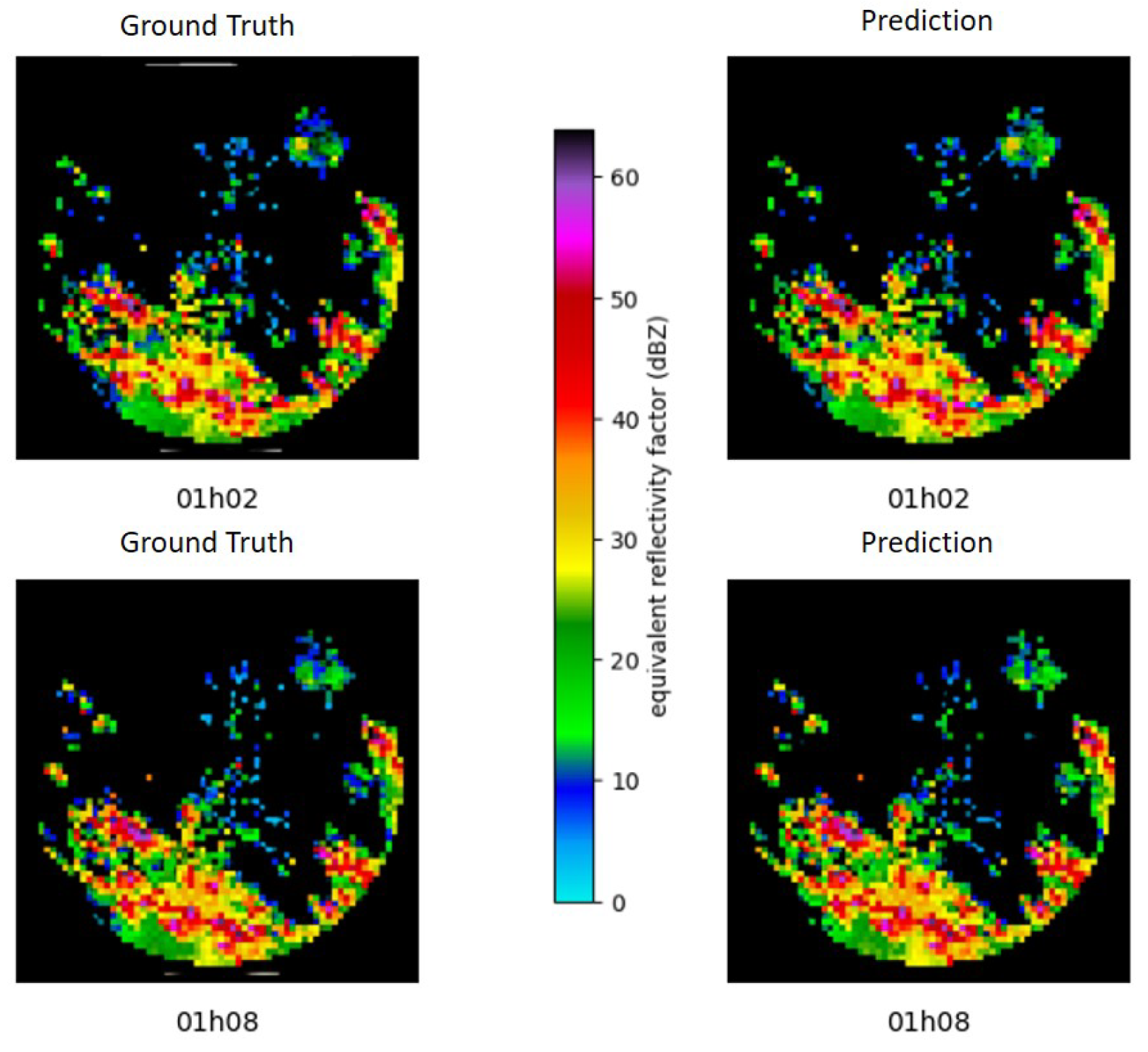
Figure 13.
Forecast for June 12, 2018, between 01:14 AM and 01:20 AM.
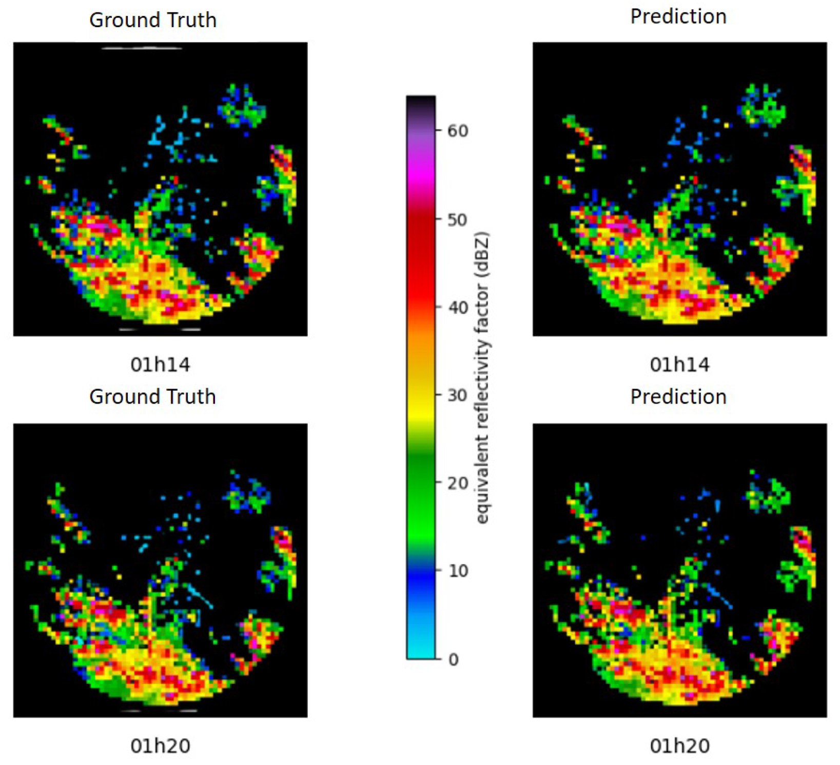
Figure 14.
Forecast for June 12, 2018, between 01:26 AM and 01:32 AM.
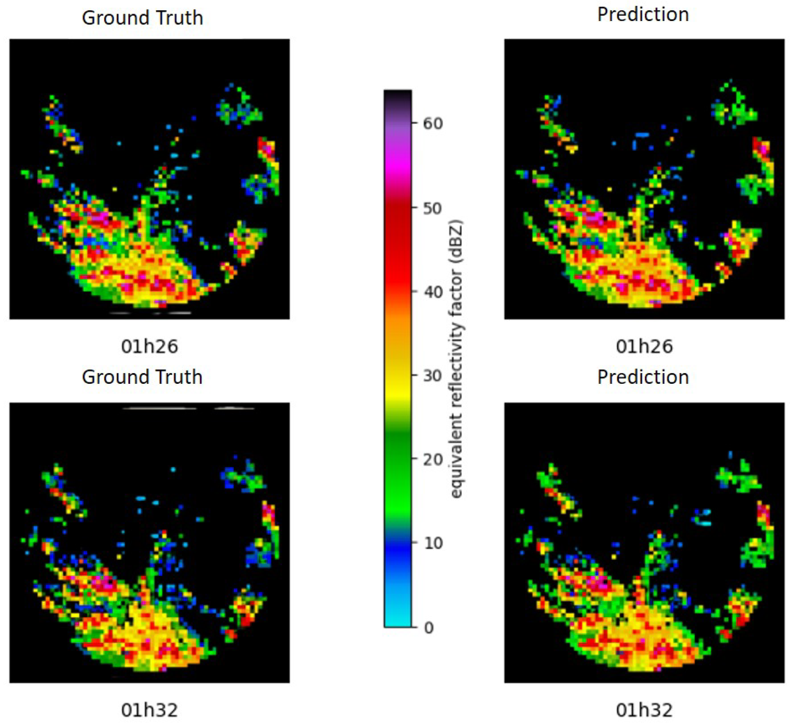
Figure 15.
Forecast for June 12, 2018, between 01:38 AM and 01:44 AM.
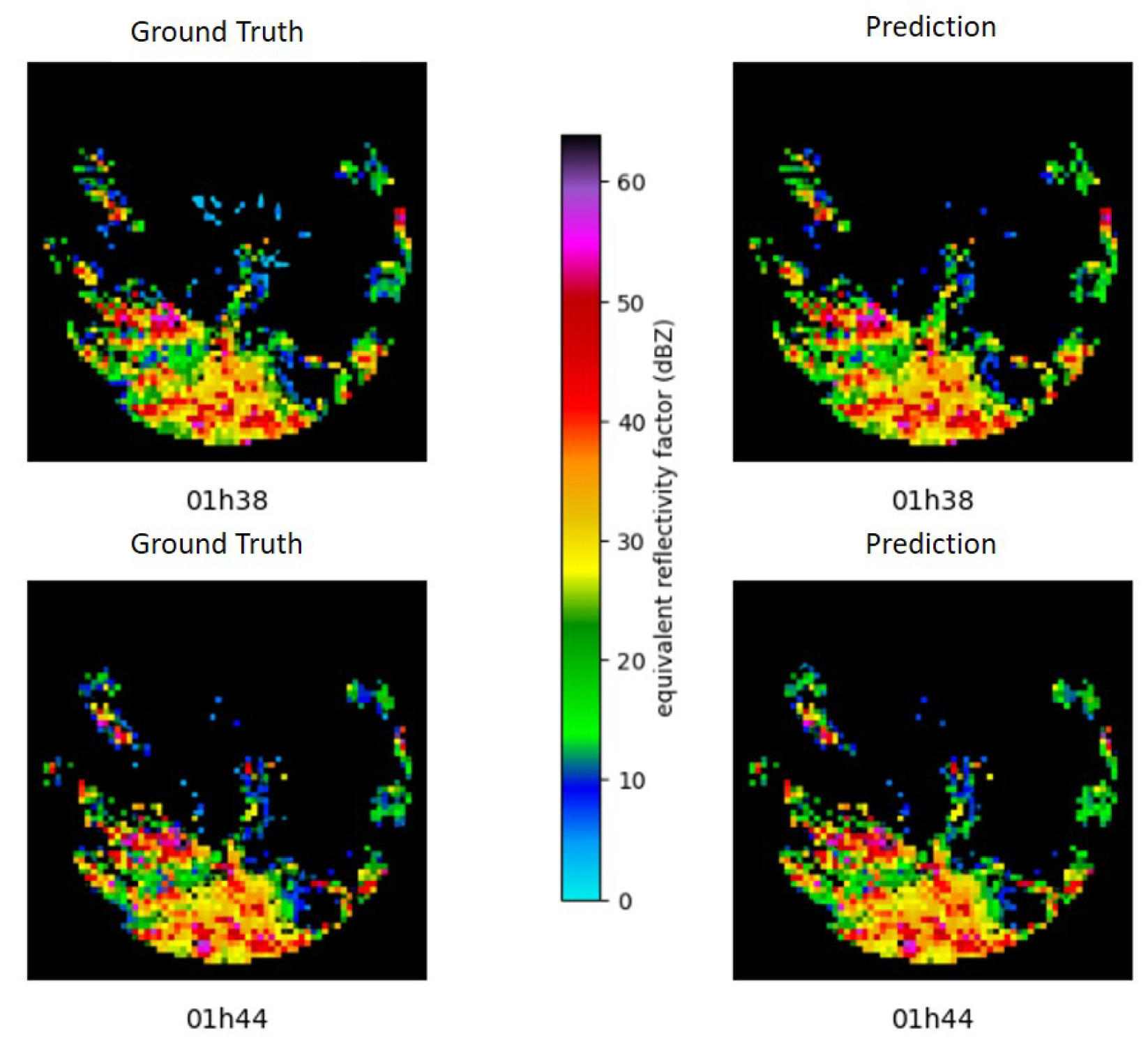
Figure 16.
Forecast for June 12, 2018, between 01:50 AM and 01:56 AM.
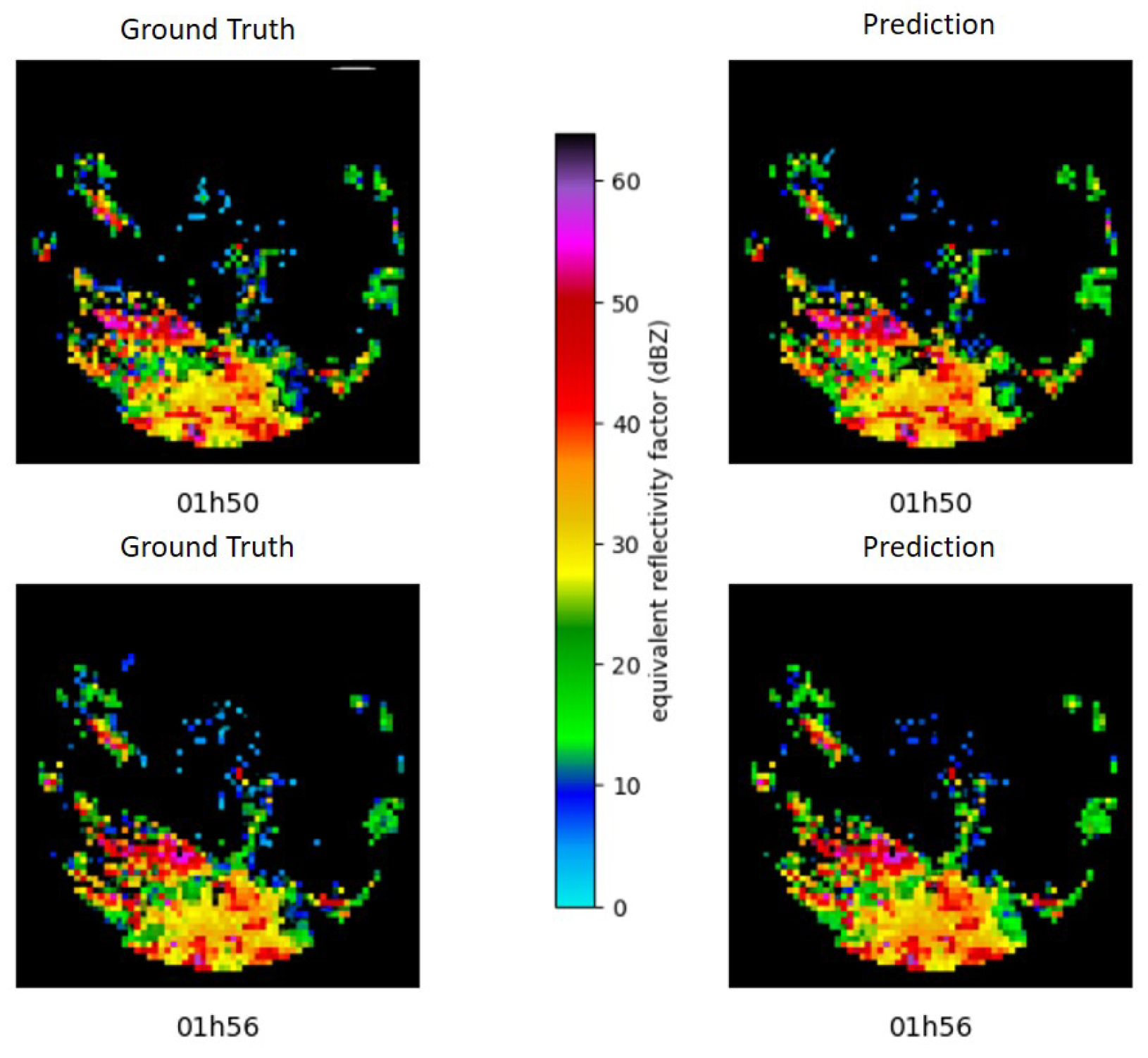
The statistics presented in Table 2 are in agreement with reflectivity factors presents in Figure 13 and Figure 16, such that the errors reproduced by the forecasting are relatively small. This coherence between the predictions resulted from neural model and the the reference is an indication that PredRNN++ is a able to learn and represents the complexity of the weather system in nowcasting scale.
4.3. Nowcasting by PredRNN++ to Chapecó Region at June 12, 2018 from 02h02 to 02h56
Figure 17, shown images from the Chapecó-SC radar from 02:02 to 02:56 on June 12, 2018. At that moment, it can be observed that the squall lines are disorganized, and there are deep convection cells distributed in the radar domain approaching the antenna.
In the figures below (Figure 18 and Figure 22, it is observed that the neural network after almost 3 hour leading time reproduces the transalation and rotation movements that occurred in the observed system.
Figure 18.
Forecast for June 12, 2018, between 02:02 AM and 02:06 AM.
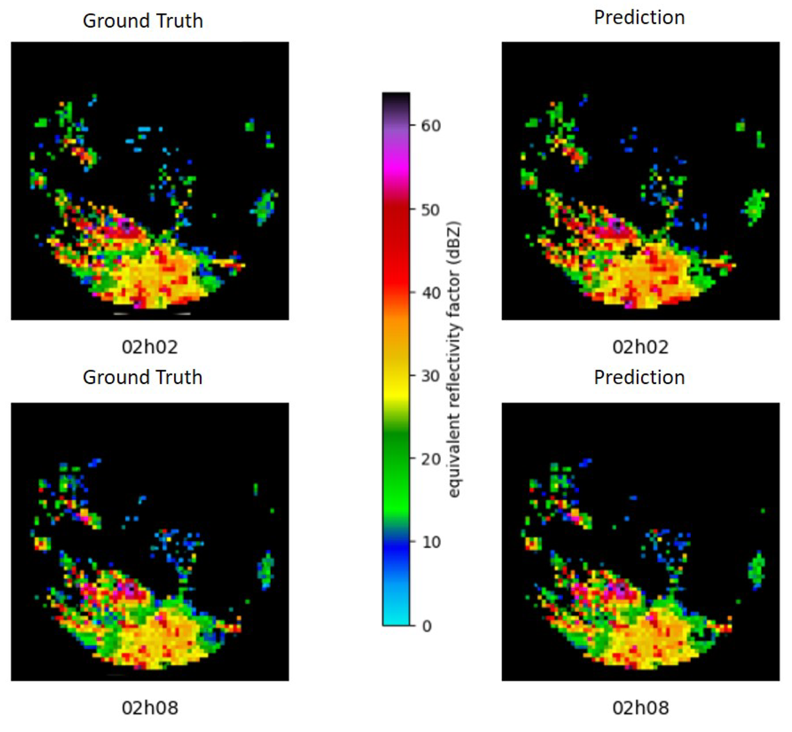
Figure 19.
Forecast for June 12, 2018, between 02:14 AM and 02:20 AM.
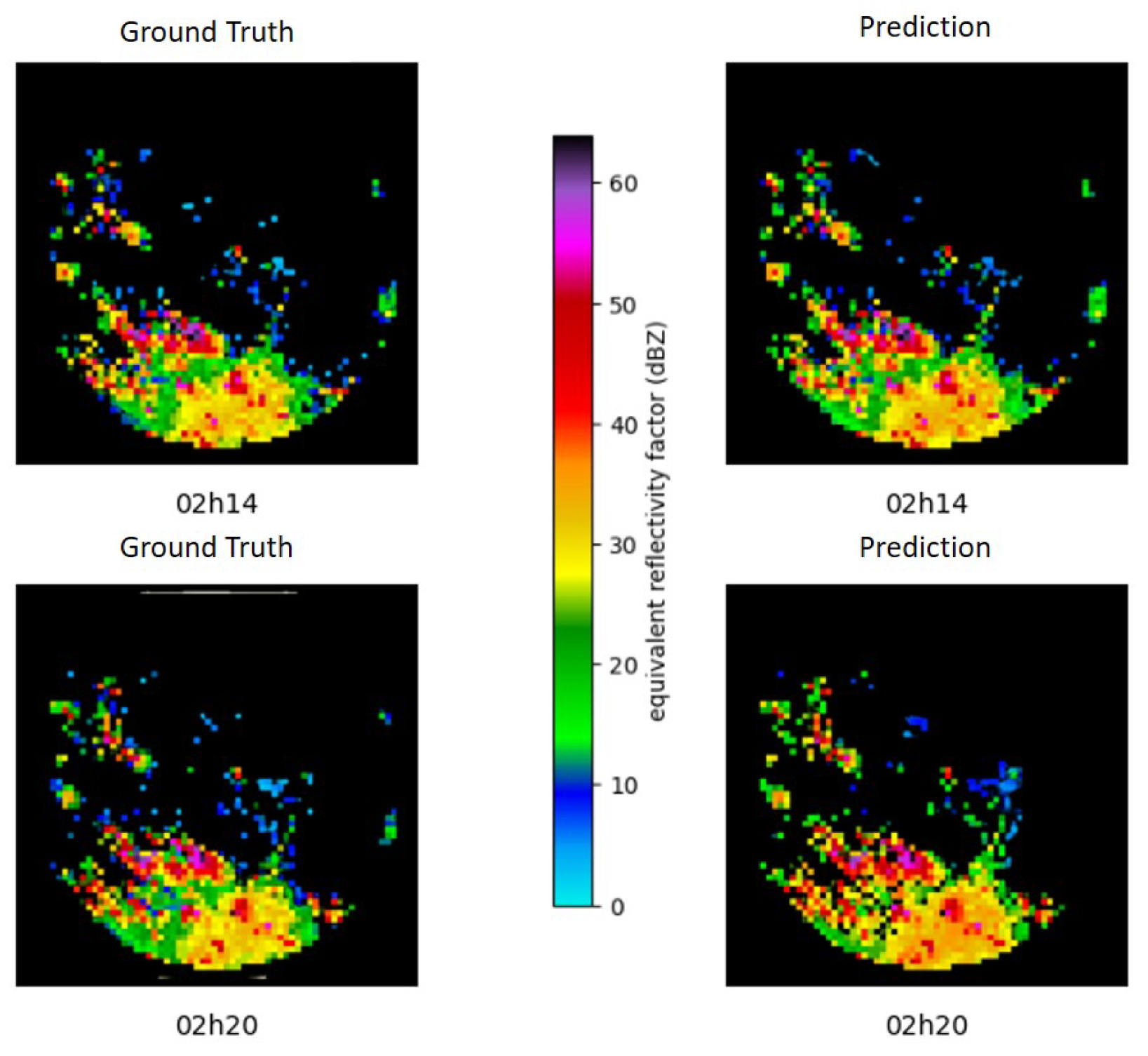
Figure 20.
Forecast for June 12, 2018, between 02:26 AM and 02:32 AM.
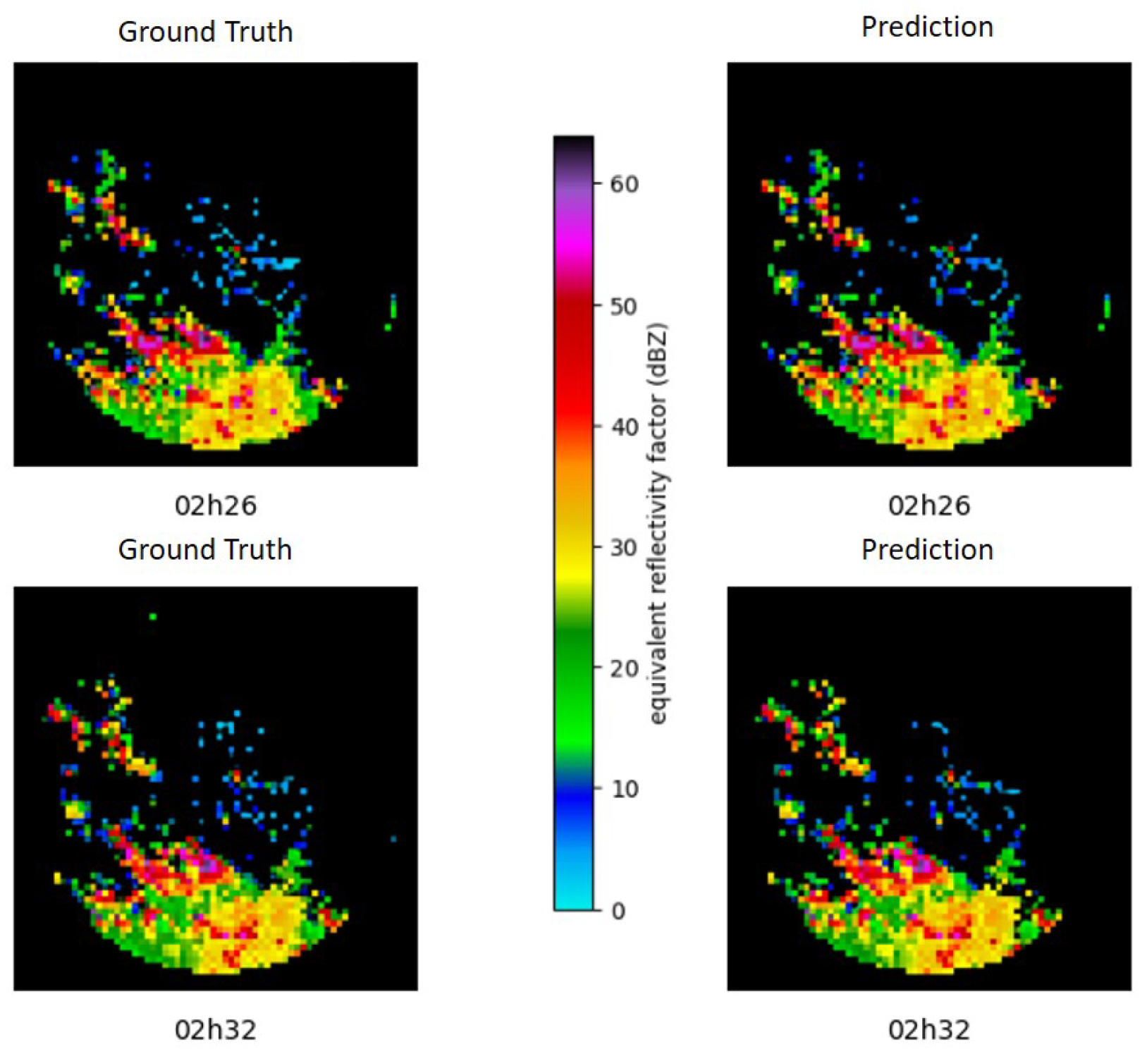
Figure 21.
Forecast for June 12, 2018, between 02:38 AM and 02:44 AM.
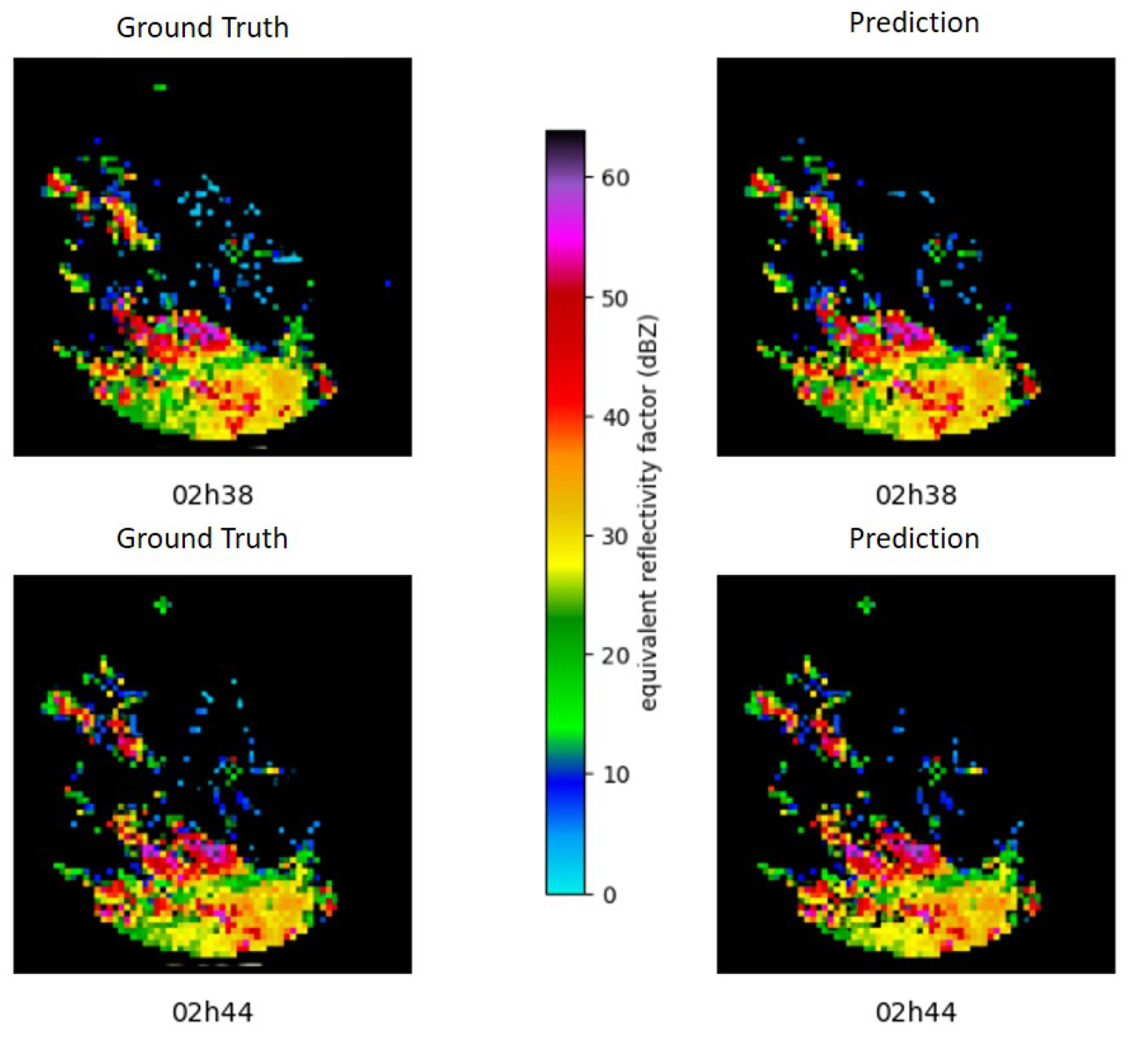
Figure 22.
Forecast for June 12, 2018, between 02:50 AM and 02:56 AM.
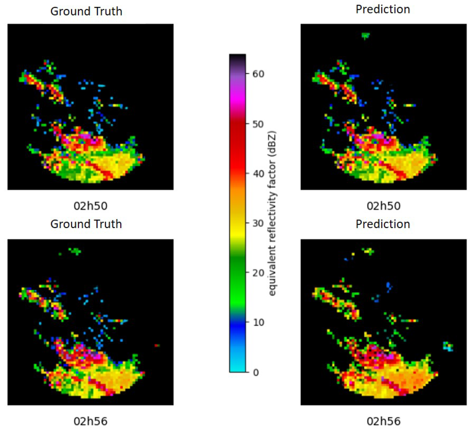
The Table 3 demonstrates that the errors remain in the same order of magnitude compared to the values observed in the previous two hours, however its oscillate, and the MAE seems to be so sensitive to the outliers as RMSE.
Despite this, SSIM values continue to show the high similarity between the model predictions and the ground truth. This persistent similarity is a strong indication that the Neural Model is capturing crucial aspects of the weather system, even in the face of oscillation in the other error indicators.
4.4. Nowcasting by PredRNN++ to Chapecó Region at June 12, 2018 from 03h02 to 03h56
Figure 23, presents images from the Chapecó-SC radar from 03:02 to 03:56 on June 12, 2018. It is observed that the squall line is not well oraganized, but pixels with reflectivity greater than 40 dBZ remain active, suggesting the existence of significant cores of convective cells.
It is presents from Figure 24, Figure 25, Figure 26, Figure 27 and Figure 28 that a nucleus of greater reflectivity appears between the precipitating cells, which manifests itself with a considerable amount of precipitation, ranging from moderate to strong, mainly in the southern region, close to the radar antenna. The remarkable correspondence between the visual observations and the neural model results reinforces the consistent accuracy of the generated predictions.
In the error analysis, shown in Table 4, the low RMSE stands out again, which is an indication of the model’s ability to keep forecasting errors in low levels. However, it becomes evident once again that RMSE and MAE are sensitive to outliers. The sensitivity and outliers of these two metrics reinforce the importance of a more empirical analysis of predictions to gain a complete understanding of model performance.
It is worth noting that the SSIM values continue to provide a positive assessment of model performance. With over 87% similarity to the terrestrial truth, the predictions generated by the neural model retain a visual and structural quality that remarkably aligns with actual observations.
5. Discussion
Theoretically, the weather forecasting has good accuracy in a 15 days leading time, limited by chaotic nature of the atmosphere. However, nowcasting weather forecasting (the first 6 hours leading time) has poor skill, because the atmospheric models takes some time to come into dynamic balance. Therefore, this research intends to propose a alternative to prediction on this scale of time [11].
Thus, in this research a neural network is proposed to overcome this problem. Specifically, a PredNN++ neural network is applied. It is a model that includes recurrent neurons and is capable of handling large amounts of data, due to the convolutional nature of this architecture.
In this work, PredNN++ is trained with data 20.000 images of meteorological radar located in south of Brazil and the results shown that the network reach a 90 % of accuracy for 50 minutes leading time. Comparing with the original work on PredRNN++, which involved training the network with approximately 108.000 images, and a comparable study [12] utilizing the same network for nowcasting in Brazil, trained with 87.500 images, it can be concluded that the results achieved were highly satisfactory.
The authors are motivated to focus future research directions on increasing the leading time to 3 hours, training PredRNN++ with a large database including satellite images, and exploring more complexy neural network structures.
Author Contributions
Conceptualization, E.H.S and F.P.H; methodology, F.C.R.; software, F.C.R.; validation, F.C.R.; formal analysis, L.C.; investigation, F.C.R; resources, L.C; data curation, F.C.R; writing—original draft preparation, F.P.H; writing—review and editing, F.P.H; visualization, F.C.R; supervision, F.P.H and E.H.S.; project administration, L.C; funding acquisition, L.C. All authors have read and agreed to the published version of the manuscript.
Funding
This research was funded by Companhia Paulista de Força e Luz (CPFL), P&D Project PD-05785-2007/2020.
Data Availability Statement
The original contributions presented in the study are included in the article; further inquiries can be directed to the corresponding author.
Conflicts of Interest
The authors declare no conflicts of interest.
Abbreviations
The following abbreviations are used in this manuscript:
| PredRNN++ | Multidisciplinary Digital Publishing Institute ++ |
| RNCR | Recurrent Convolutional Neural Network |
| ML | Machine Learning |
References
- Toth, Z.; Buizza, R. Chapter 2 - Weather Forecasting: What Sets the Forecast Skill Horizon? In Sub-Seasonal to Seasonal Prediction; Robertson, A.W., Vitart, F., Eds.; Elsevier, 2019; pp. 17–45. [CrossRef]
- Conglan, C.; Mingxuan, C.; Jianjie, W.; Feng, G.; HY, Y.L. Short-term quantitative precipitation forecast experiments based on blending of nowcasting with numerical weather prediction. Acta Meteorologica Sinica 2013, 397–415. [Google Scholar] [CrossRef]
- Shi, X.; Gao, Z.; Lausen, L.; Wang, H.; Yeung, D.Y.; kin Wong, W.; chun Woo, W. Deep Learning for Precipitation Nowcasting: A Benchmark and A New Model. arXiv 2017, arXiv:1706.03458. [Google Scholar]
- Gutierrez-Corea, F.V.; Manso-Callejo, M.A.; Moreno-Regidor, M.P.; Manrique-Sancho, M.T. Forecasting short-term solar irradiance based on artificial neural networks and data from neighboring meteorological stations. Solar Energy 2016, 134, 119–131. [Google Scholar] [CrossRef]
- Daniel, L.O.; Sigauke, C.; Chibaya, C.; Mbuvha, R. Short-Term Wind Speed Forecasting Using Statistical and Machine Learning Methods. Algorithms 2020, 13, 132. [Google Scholar] [CrossRef]
- Tuyen, D.N.; Tuan, T.M.; Le, X.H.; Tung, N.T.; Chau, T.K.; Van Hai, P.; Gerogiannis, V.C.; Son, L.H. RainPredRNN: A New Approach for Precipitation Nowcasting with Weather Radar Echo Images Based on Deep Learning. Axioms 2022, 11, 107. [Google Scholar] [CrossRef]
- Wang, Y.; Gao, Z.; Long, M.; Wang, J.; Yu, P.S. PredRNN++: Towards A Resolution of the Deep-in-Time Dilemma in Spatiotemporal Predictive Learning. arXiv 2018, arXiv:1804.06300. [Google Scholar]
- Holton, J.R. An introduction to dynamic meteorology. American Journal of Physics 1973, 41, 752–754. [Google Scholar] [CrossRef]
- Bluestein, H.B. Synoptic-dynamic Meteorology in Midlatitudes: Observations and theory of weather systems; Taylor & Francis: New York, NY, USA, 1992; Volume 2. [Google Scholar]
- Lopes, M.M.; Nascimento, E.L. Use of remote sensing via satellite in the identification of tornado damage paths in a severe weather event in Rio Grande do Sul. Ciência Natura 2020, 42. [Google Scholar] [CrossRef]
- Browning, K.; Collier, C. Nowcasting of precipitation systems. Reviews of Geophysics 1989, 27, 345–370. [Google Scholar] [CrossRef]
- Bonnet, S.M.; Evsukoff, A.; Morales Rodriguez, C.A. Precipitation Nowcasting with Weather Radar Images and Deep Learning in São Paulo, Brasil. Atmosphere 2020, 11, 1157. [Google Scholar] [CrossRef]
| 1 | Here, we refer to all individuals without scientific knowledge on the subject |
Figure 1.
Damaged transmission line.
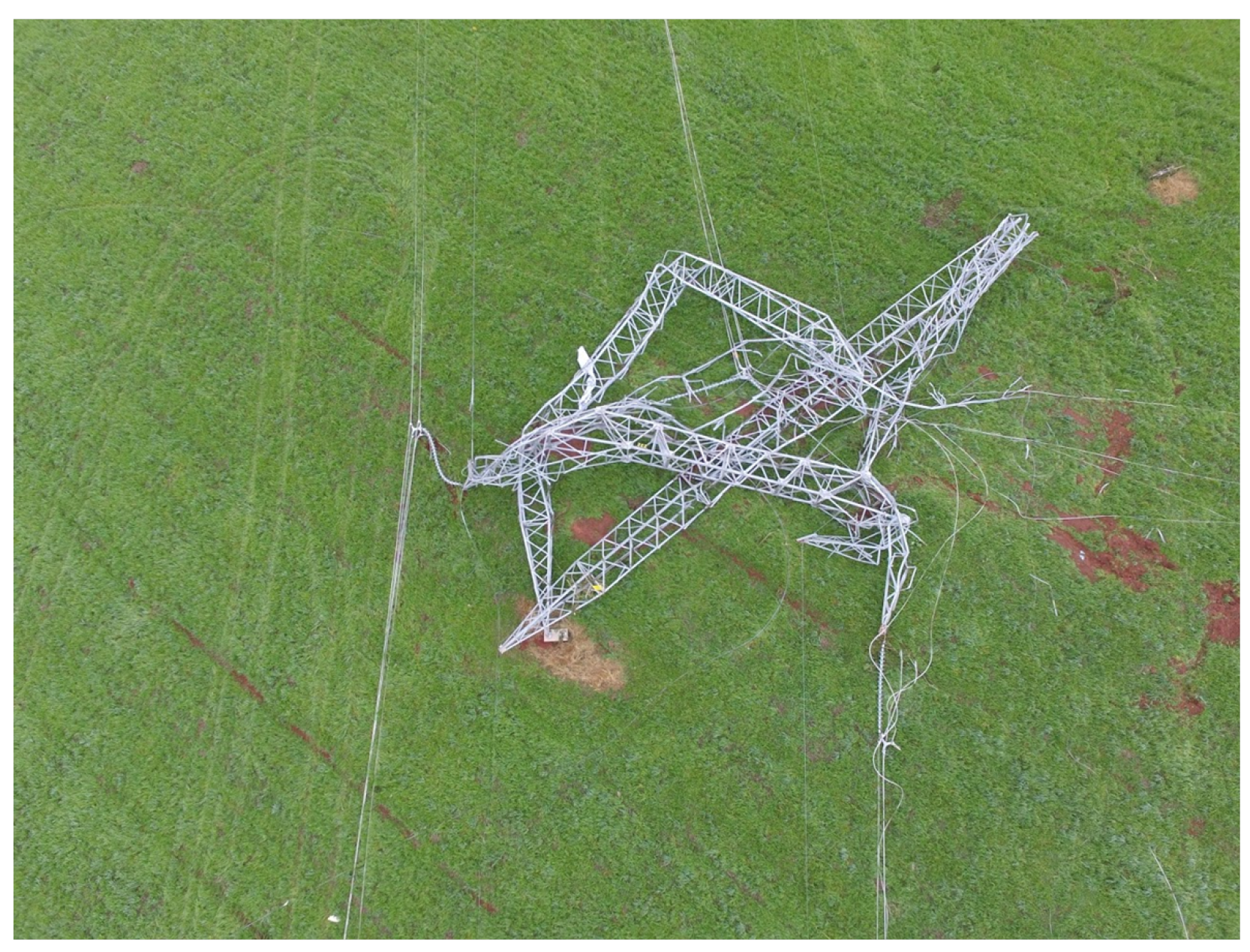
Figure 2.
Satellite images at 00:15 AM, 00:30 AM, and 00:45 AM on June 12, 2018.
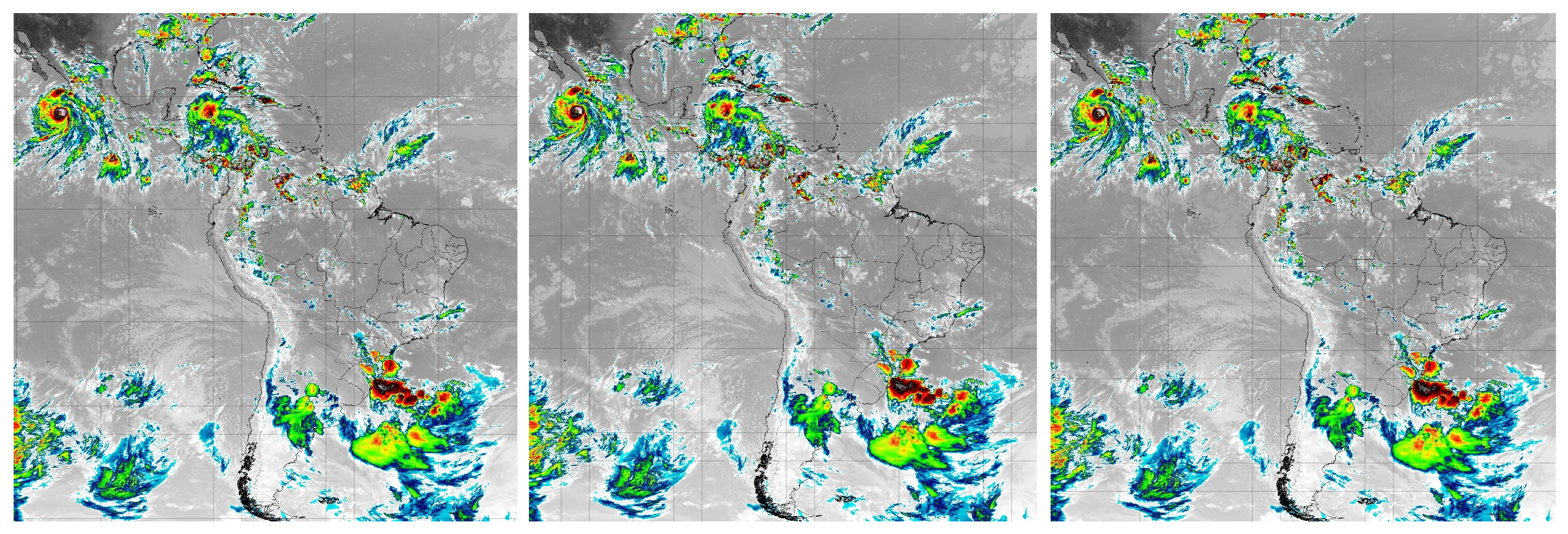
Figure 3.
Surface variable fields on June 11, 2018 at 6:00 PM and on June 12, 2018 at 12:00 PM and at 12:06 PM.
Figure 3.
Surface variable fields on June 11, 2018 at 6:00 PM and on June 12, 2018 at 12:00 PM and at 12:06 PM.
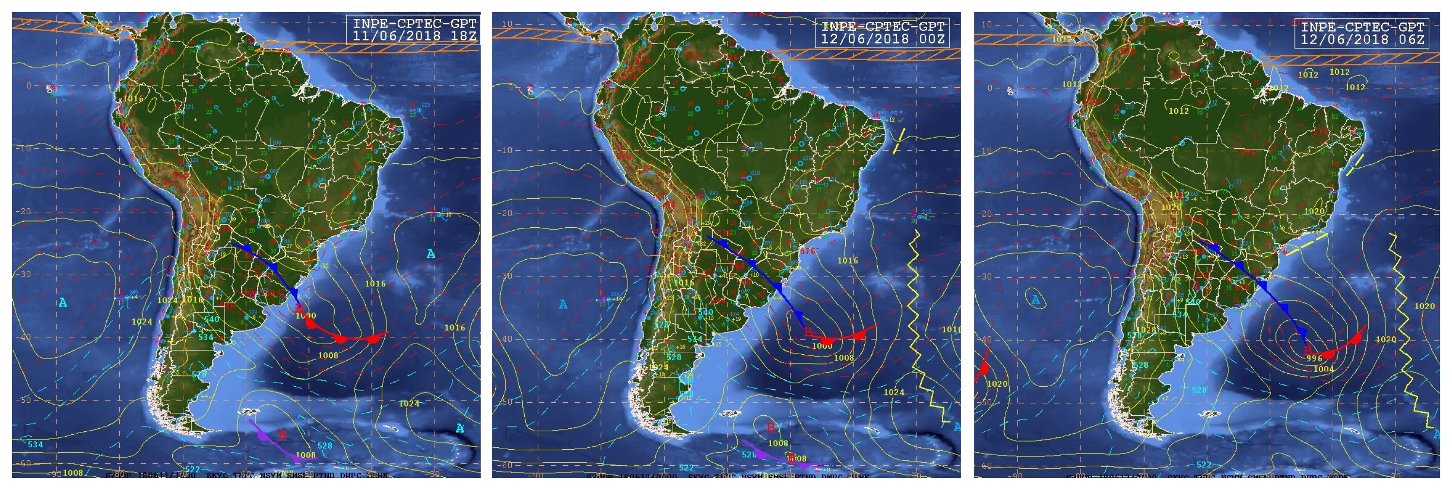
Figure 4.
Altitude variable fields on June 11, 2018, at 6:00 PM and on June 12, 2018, at 12:00 PM and at 12:06 PM.
Figure 4.
Altitude variable fields on June 11, 2018, at 6:00 PM and on June 12, 2018, at 12:00 PM and at 12:06 PM.

Figure 5.
Images from the Chapecó-SC radar between 11:02 PM and 11:56 PM on June 11, 2018.
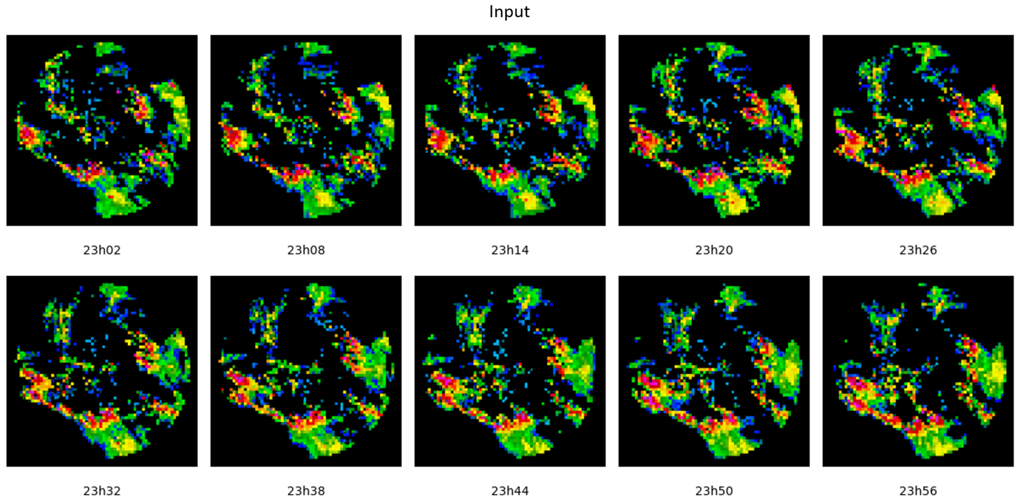
Figure 6.
Forecast for June 12, 2018, between 12:02 AM and 12:08 AM.
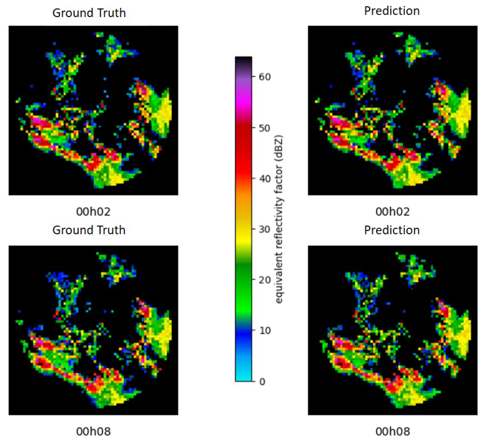
Figure 7.
Forecast for June 12, 2018, between 12:14 AM and 12:20 AM.
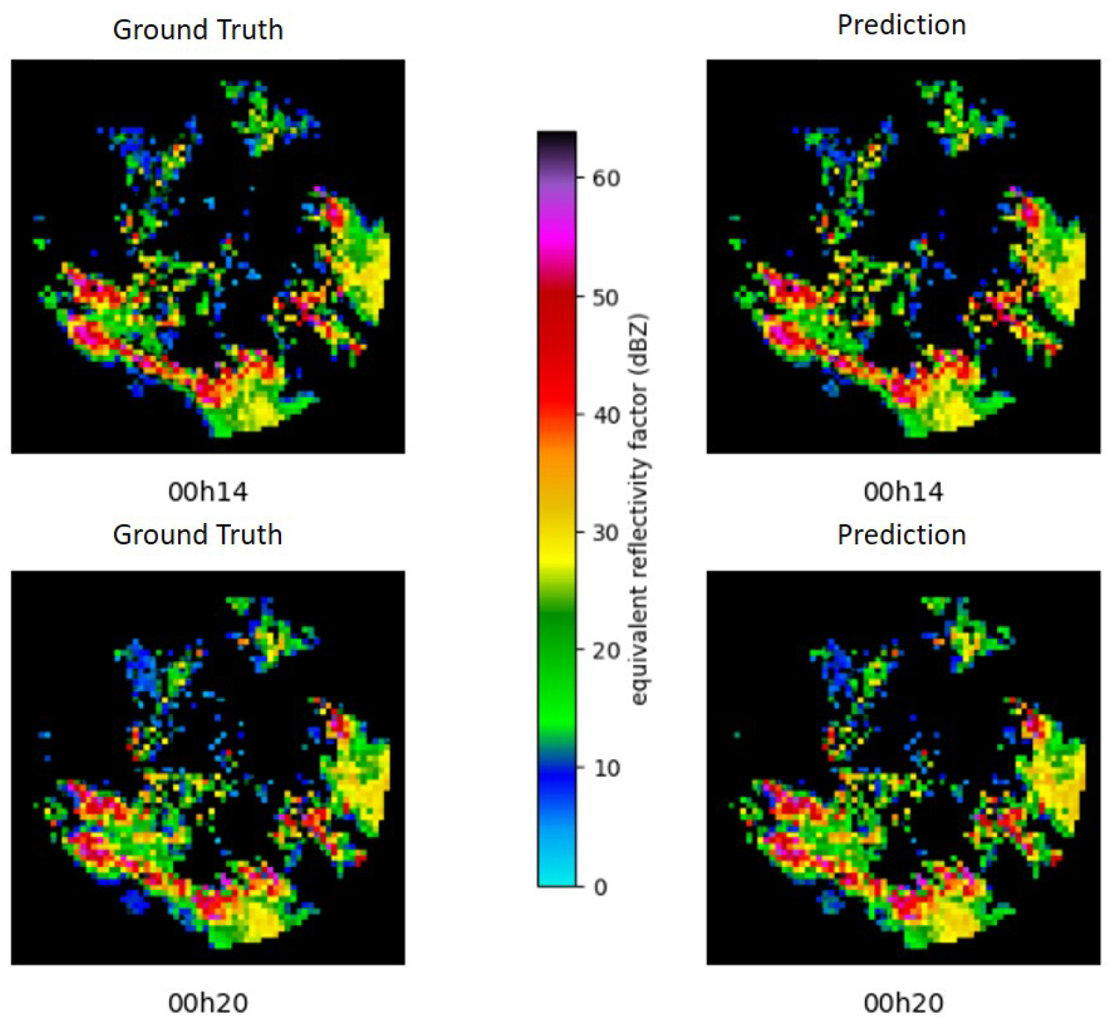
Figure 8.
Forecast for June 12, 2018, between 12:26 AM and 12:32 AM.
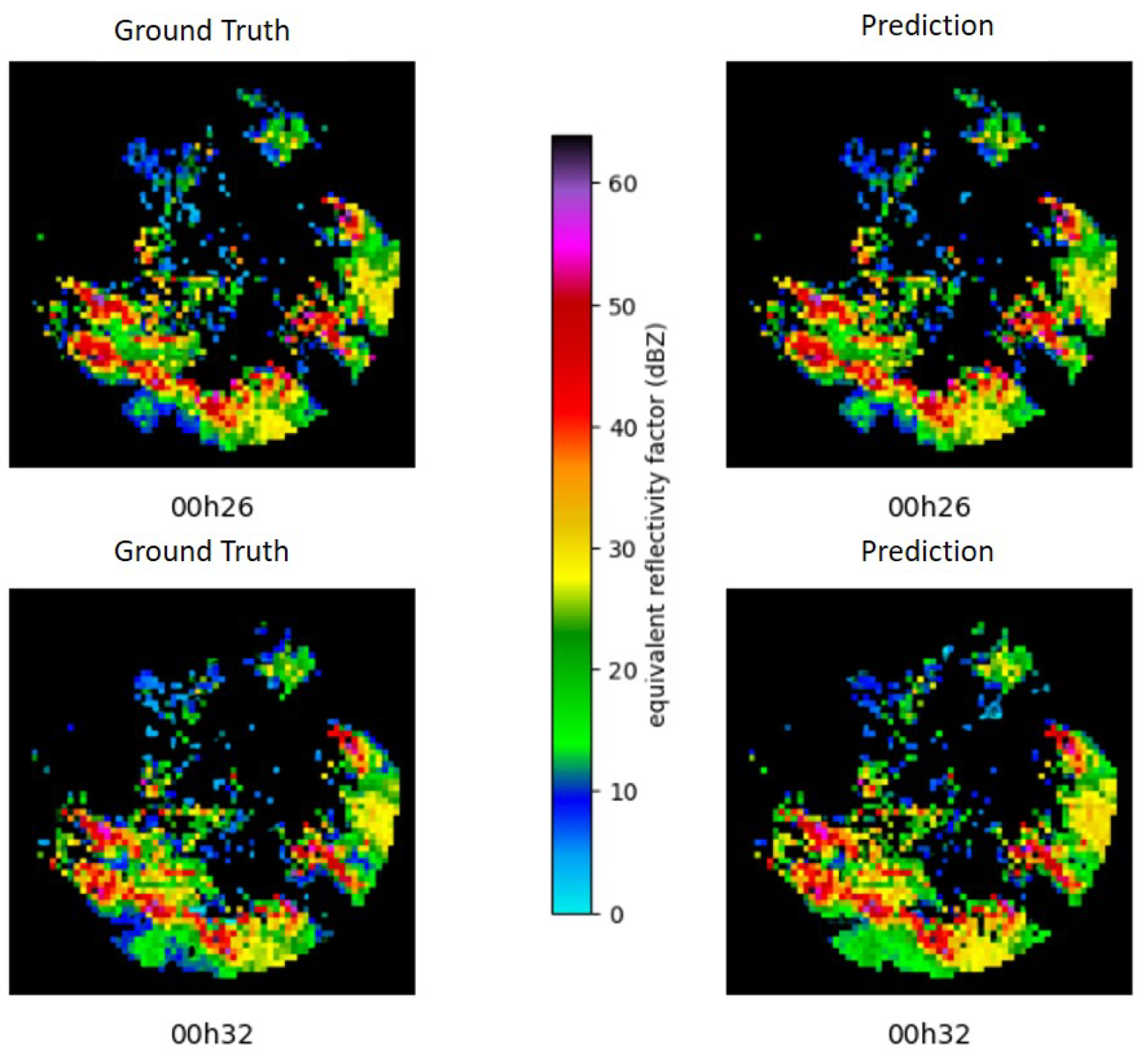
Figure 9.
Forecast for June 12, 2018, between 12:38 AM and 12:44 AM.
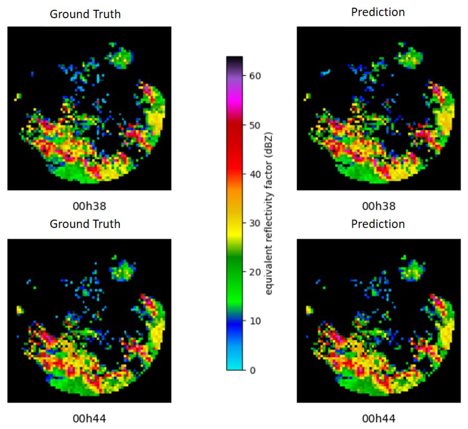
Figure 10.
Forecast for June 12, 2018, between 12:50 AM and 12:56 AM.
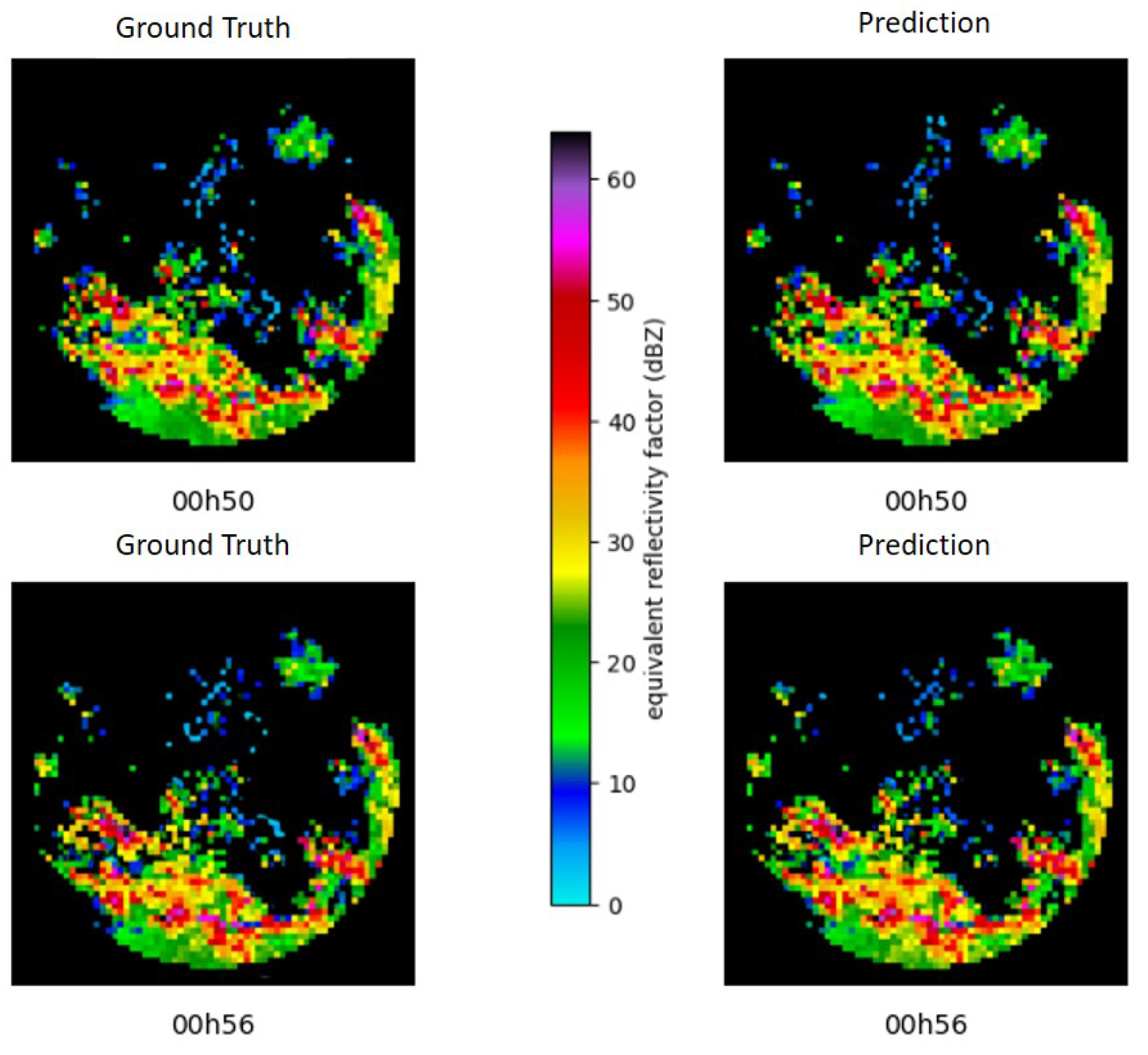
Figure 11.
Images from the Chapecó-SC radar between 00:02 and 00:56 on June 12, 2018.
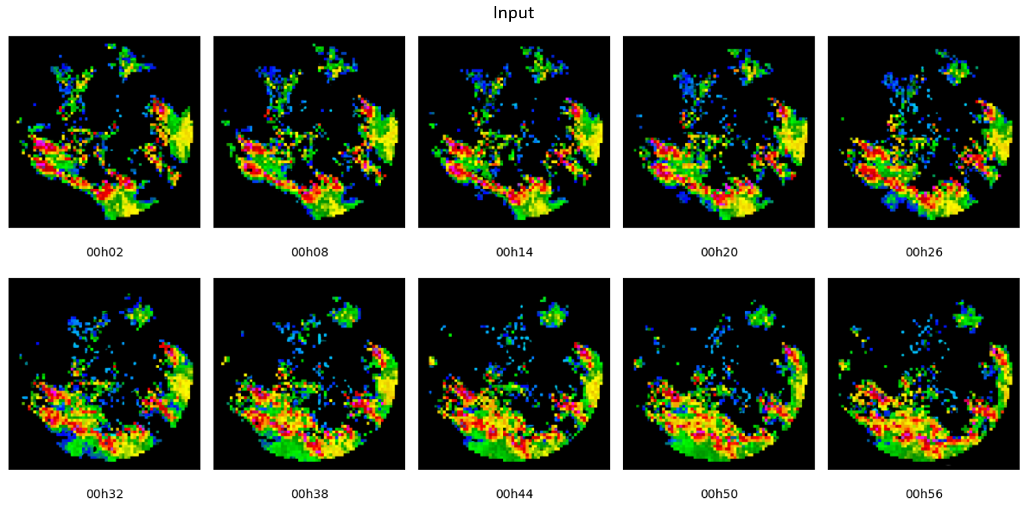
Figure 17.
Images from the Chapecó-SC radar between 01:02 and 01:56 on June 12, 2018.
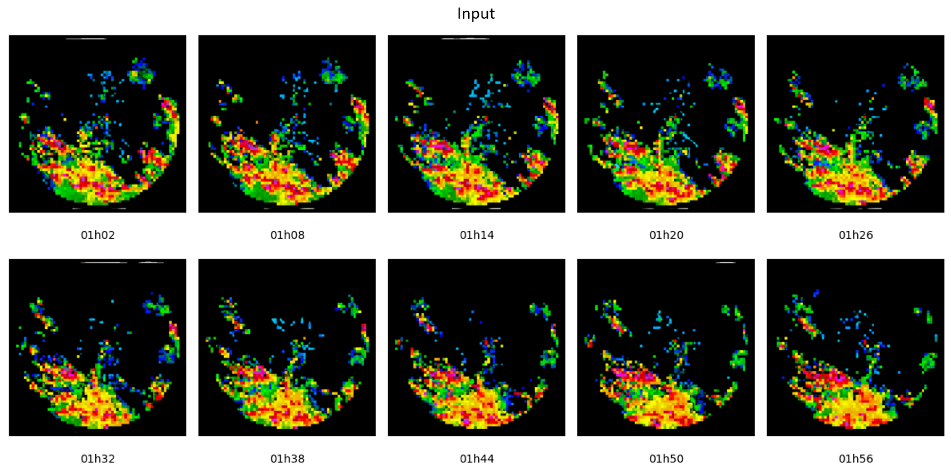
Figure 23.
Images from the Chapecó-SC radar between 02:02 and 02:56 on June 12, 2018.
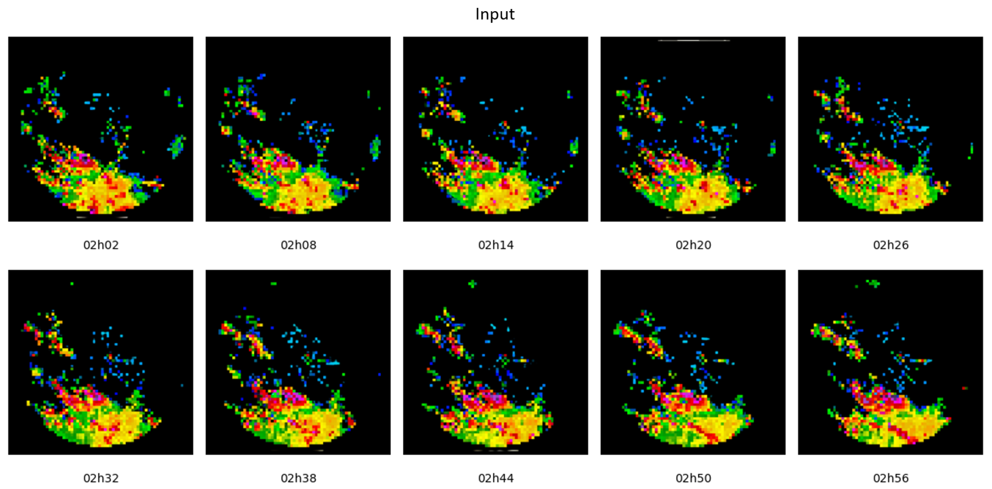
Figure 24.
Forecast for June 12, 2018, between 03:02 AM and 03:06 AM.
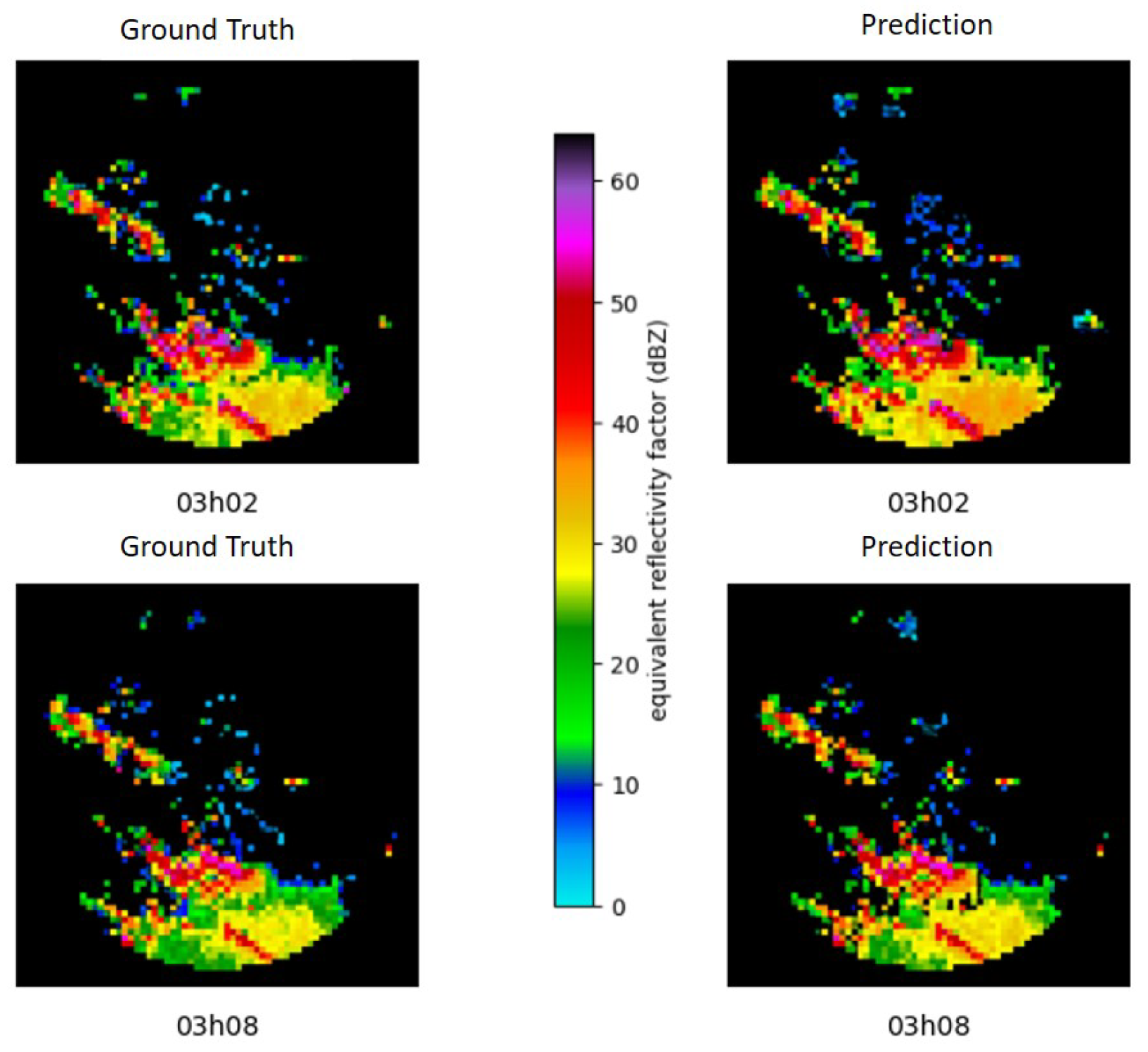
Figure 25.
Forecast for June 12, 2018, between 03:14 AM and 03:20 AM.
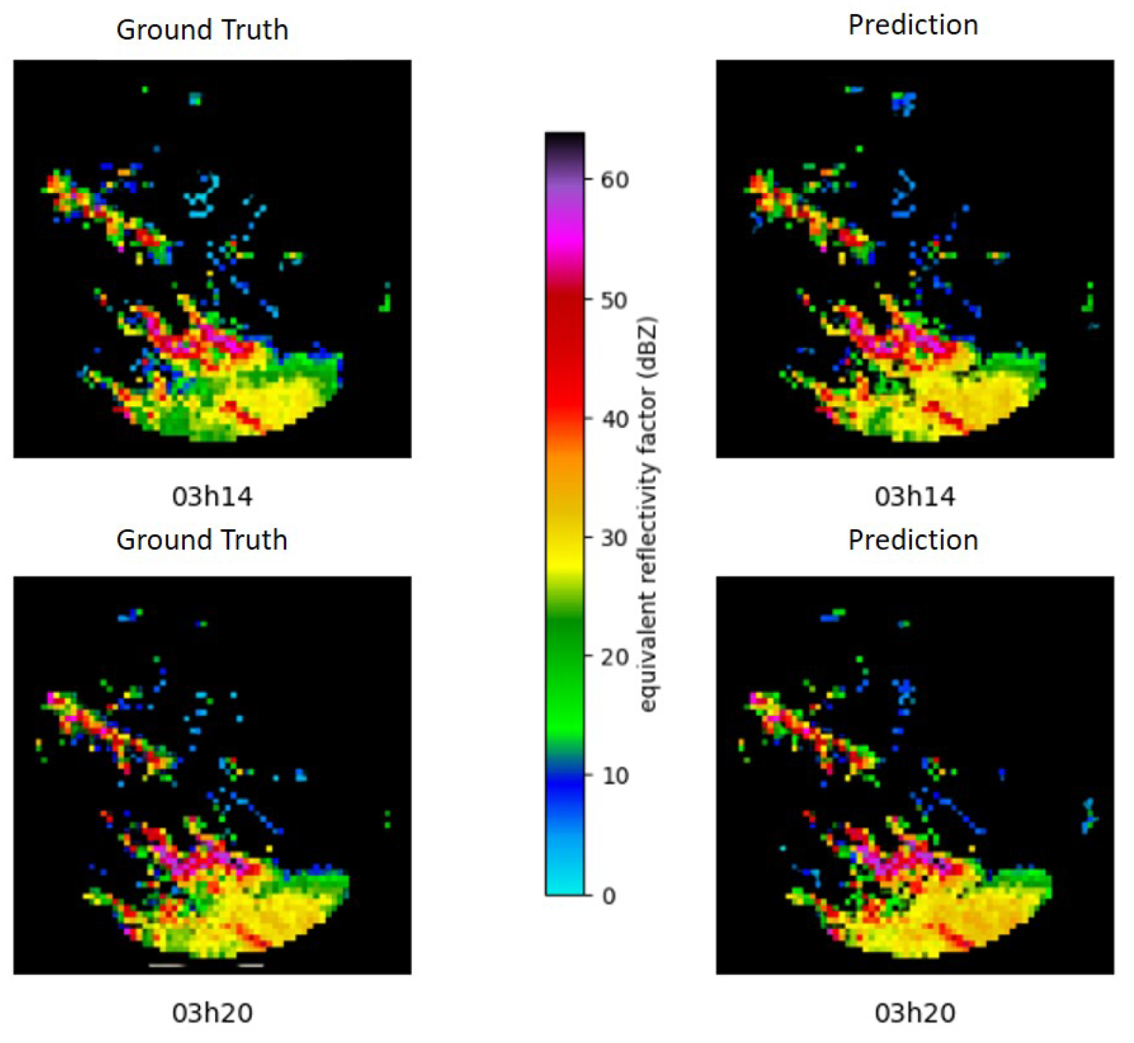
Figure 26.
Forecast for June 12, 2018, between 03:26 AM and 03:32 AM.
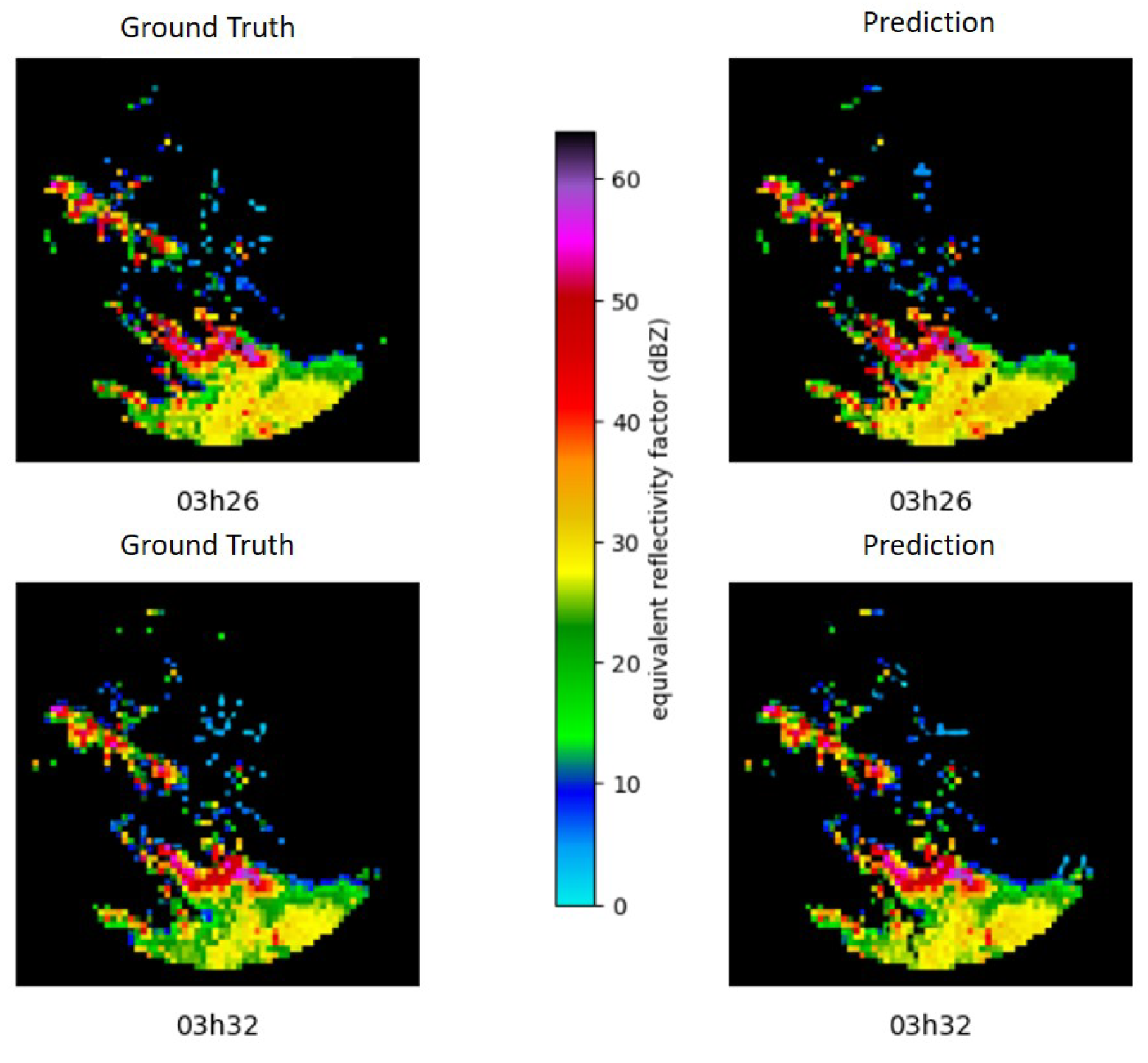
Figure 27.
Forecast for June 12, 2018, between 03:38 AM and 03:44 AM.
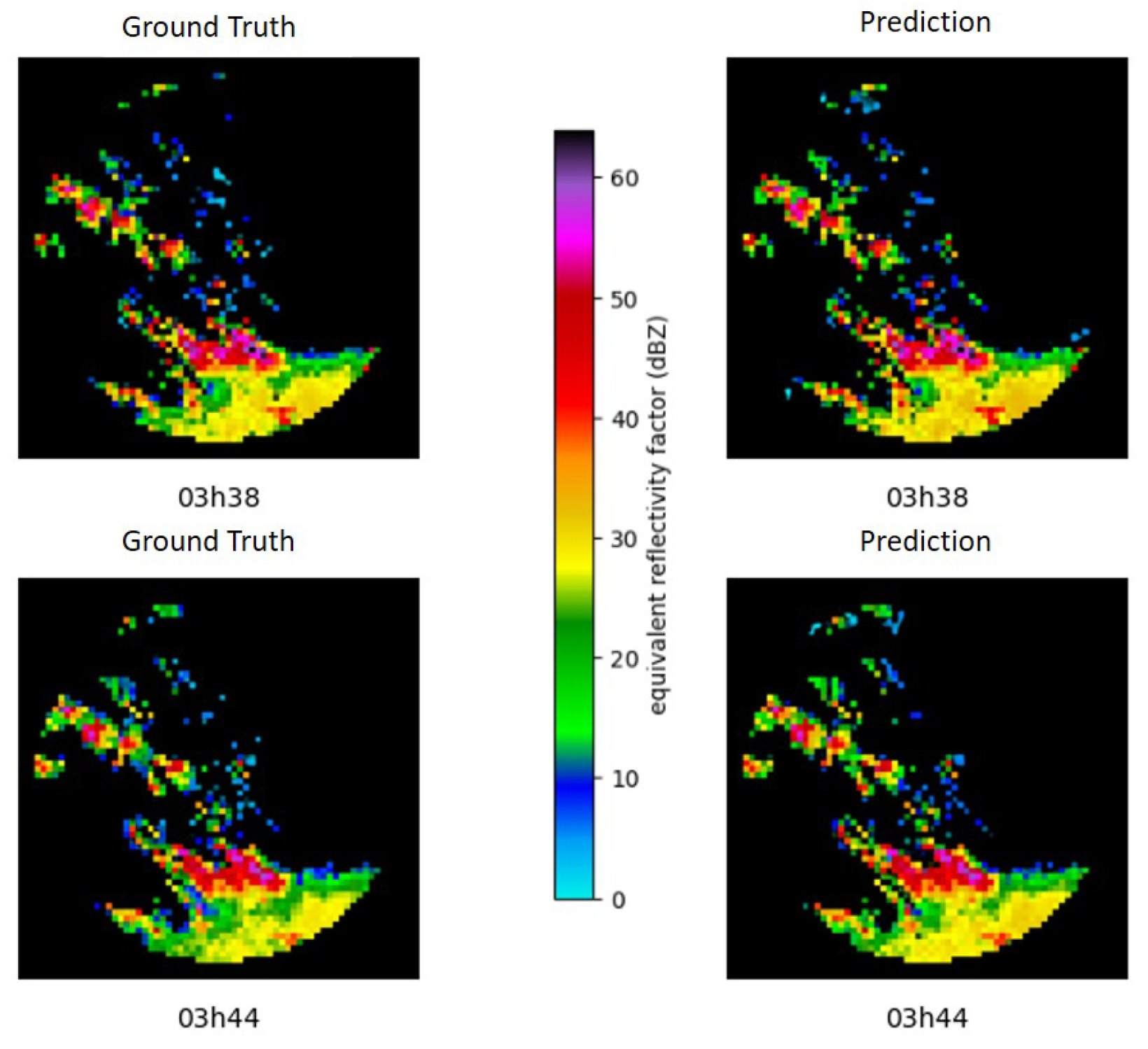
Figure 28.
Forecast for June 12, 2018, between 03:50 AM and 03:56 AM.
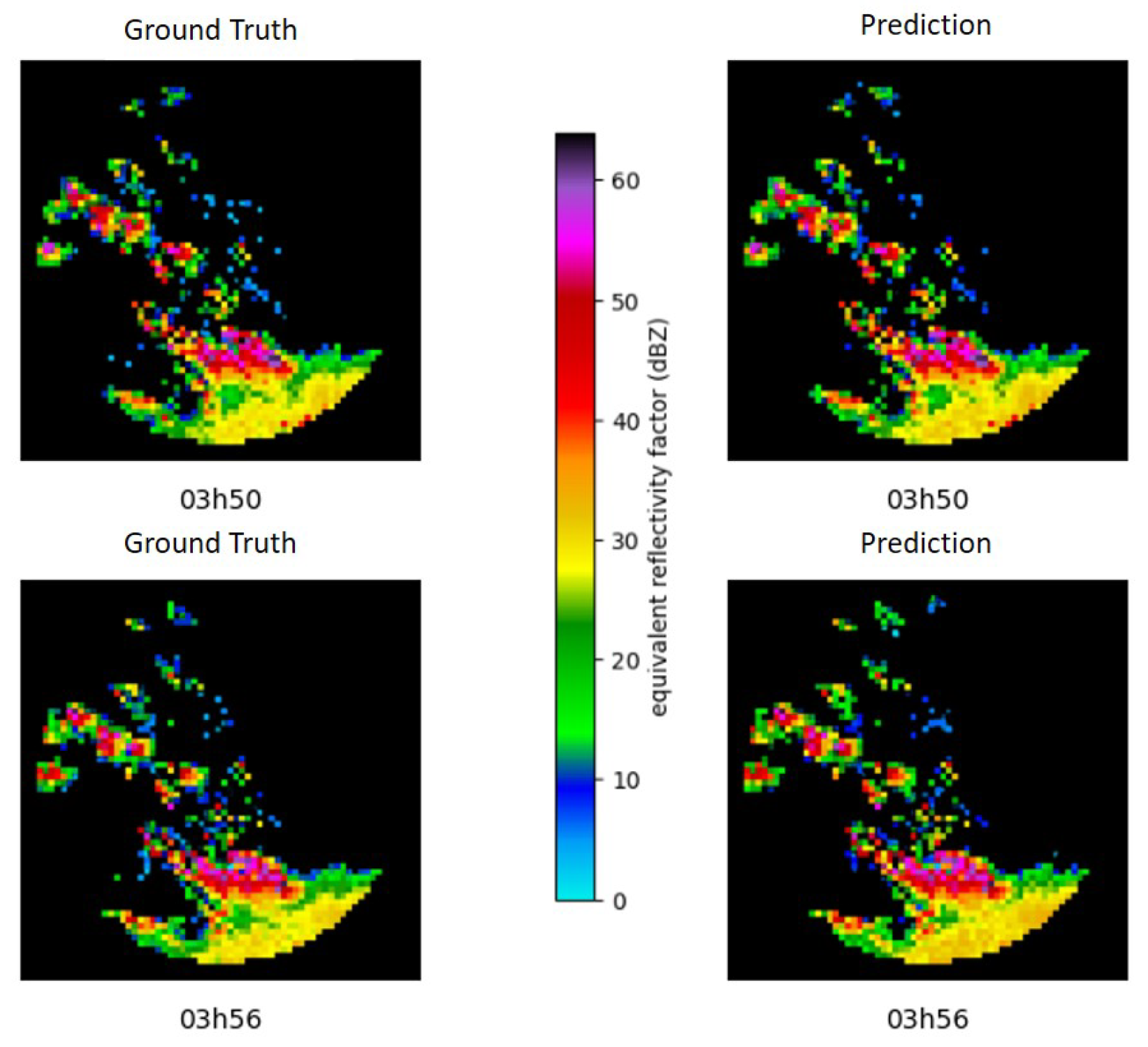

Table 1.
Statistic from 00h02 to 00h56.
| Time | RMSE | SSIM | MAE |
|---|---|---|---|
| 00h02 | 12,97092 | 0,88736 | 21,46726 |
| 00h08 | 13,89034 | 0,87895 | 22,08349 |
| 00h14 | 13,57018 | 0,88225 | 21,84790 |
| 00h20 | 13,26058 | 0,88474 | 21,79353 |
| 00h26 | 12,83015 | 0,88791 | 21,61334 |
| 00h32 | 15,78007 | 0,86003 | 23,67804 |
| 00h38 | 13,41088 | 0,88346 | 21,19067 |
| 00h44 | 12,61092 | 0,88971 | 22,47739 |
| 00h50 | 12,62077 | 0,88989 | 20,52912 |
| 00h56 | 13,30041 | 0,88507 | 22,25039 |
Table 2.
Statistic from 01h02 to 01h56.
| Horário | RMSE | SSIM | MAE |
|---|---|---|---|
| 01h02 | 13,52034 | 0,88278 | 21,9971 |
| 01h08 | 13,04095 | 0,88647 | 21,5225 |
| 01h14 | 14,10028 | 0,87684 | 22,0324 |
| 01h20 | 14,87017 | 0,87007 | 21,2735 |
| 01h26 | 14,58071 | 0,87317 | 22,8742 |
| 01h32 | 14,91060 | 0,86901 | 21,8854 |
| 01h38 | 13,85078 | 0,88070 | 20,8620 |
| 01h44 | 13,05048 | 0,88653 | 20,7215 |
| 01h50 | 13,61079 | 0,88159 | 20,84084 |
| 01h56 | 13,94063 | 0,87954 | 20,32897 |
Table 3.
Statistics from 02h02 to 02h56.
| Horário | RMSE | SSIM | MAE |
|---|---|---|---|
| 02h02 | 14,39014 | 0,87526 | 20,64813 |
| 02h08 | 12,43389 | 0,89125 | 18,00123 |
| 02h14 | 13,79503 | 0,88110 | 20,2910 |
| 02h20 | 16,53102 | 0,85365 | 22,2797 |
| 02h26 | 12,37876 | 0,89158 | 18,56445 |
| 02h32 | 12,63045 | 0,88983 | 18,44449 |
| 02h38 | 12,90621 | 0,88707 | 19,65196 |
| 02h44 | 12,18933 | 0,89234 | 18,96536 |
| 02h50 | 12,76207 | 0,88934 | 19,05172 |
| 02h56 | 15,96798 | 0,86363 | 21,43082 |
Table 4.
Métricas entre 03h02 e 03h56.
| Horário | RMSE | SSIM | MAE |
|---|---|---|---|
| 03h02 | 15,38004 | 0,86830 | 20,2442 |
| 03h08 | 13,63203 | 0,88250 | 19,78822 |
| 03h14 | 14,65815 | 0,87501 | 21,0617 |
| 03h20 | 13,81097 | 0,88143 | 19,55957 |
| 03h26 | 13,32601 | 0,88579 | 20,98579 |
| 03h32 | 13,29928 | 0,88535 | 19,82172 |
| 03h38 | 13,60506 | 0,88224 | 18,71355 |
| 03h44 | 14,02310 | 0,87950 | 20,9835 |
| 03h50 | 12,96742 | 0,88728 | 19,43241 |
| 03h56 | 14,02159 | 0,87896 | 20,4681 |
Disclaimer/Publisher’s Note: The statements, opinions and data contained in all publications are solely those of the individual author(s) and contributor(s) and not of MDPI and/or the editor(s). MDPI and/or the editor(s) disclaim responsibility for any injury to people or property resulting from any ideas, methods, instructions or products referred to in the content. |
© 2024 by the authors. Licensee MDPI, Basel, Switzerland. This article is an open access article distributed under the terms and conditions of the Creative Commons Attribution (CC BY) license (http://creativecommons.org/licenses/by/4.0/).
Copyright: This open access article is published under a Creative Commons CC BY 4.0 license, which permit the free download, distribution, and reuse, provided that the author and preprint are cited in any reuse.


