
Submitted:
21 August 2024
Posted:
22 August 2024
You are already at the latest version
Abstract
Increasing concerns on animal welfare in commercial pig industry include aggression between pigs as it affects their health and growth. Early detection of aggressive behaviors is essential for optimizing their living environment. A major challenge for detection is that these behaviors are observed occasionally in normal conditions. Under this circumstance, a limited amount of aggressive behavior data will lead to class imbalance issue, making it difficult to develop an effective classification model for the detection of aggressive behaviors. To overcome this problem, we approach the aggressive behavior detection problem as a case of anomaly detection rather than classification and propose a model based on anomaly detection, which can better handle unbalanced class distribution and effectively detect the infrequent, aggressive episodes of pigs. The model consists of a convolutional neural network (CNN) and a variational long short-term memory (LSTM) autoencoder. Additionally, we adopted a training method similar to weakly supervised anomaly detection and included a few aggressive behavior data in the training set for prior learning. To effectively utilize the aggressive behavior data, we created Reconstruction Loss Inversion, a novel objective function, to train the autoencoder-based model to increase the reconstruction error of aggressive behaviors by inverting the loss function. Our anomaly detection approach significantly outperforms traditional classification-based methods, effectively identifying aggressive behaviors in a natural farming environment. This method offers a robust solution for detecting aggressive animal behaviors and contributes to improving their welfare.
Keywords:
Aggression detection
; Unbalanced dataset
; Autoencoder
; Computer vision
; Deep learning
1. Introduction
Increasing demand for pork products due to population growth has contributed to commercial pig market expansion [1]. Meanwhile, consumers have developed serious concerns in ethical and sustainable pork production measures [2]. Optimization of the farming environment is important for maintaining high-quality production, which leads to interest in improving animal welfare. As the importance of animal welfare increases, the industry aims to continuously monitor the farming environment and simultaneously analyze stress, injuries, and diseases in livestock [3]. Advanced technologies are required for monitoring health conditions and farming environments in pigs [4].
To ensure uniform growth, pigs are separated periodically according to growth stages. During this process, pigs establish a new hierarchical order through aggressive behavior to obtain resources in a limited living space. The aggressive behavior greatly interferes health conditions and growth of pigs, subsequently affecting production quality [5,6]. As a result, continuous behavior monitoring technology involving not humans but AI models has been steadily developed and adopted to replace traditional manual inspection in agricultural fields [7,8,9,10,11,12].
Initial research on aggressive behavior involved Linear Discriminant Analysis to extract and analyze the average movement intensity from Motion History Image (MHI) data [7]. Chen and his colleagues have proposed the use of Kinect depth sensors and differences in kinetic energy for the calculation of the distance between pigs using support vector machine (SVM) [9,11]. Recently, they have proposed deep learning frameworks for classifying aggressive episodes in pigs based on convolutional neural network (CNN) and long short-term memory (LSTM) for classifying aggressive behavior, under the assumption of a balanced class distribution [12]. However, this approach is inappropriate for comparing data obtained from actual livestock farms, where aggressive behavior in pigs occurs suddenly and irregularly. Therefore, aggression data counted for only 3% of the total data in the research of Chen et al. (2019) [11]. Prior research has been conducted based on balanced data, which causes the limitation of oversampling by simply transforming the aggression data in later research [12]. In deep learning research, diverse data input is a key point for better model establishment [13]. Nevertheless, general classification models are not capable of learning a wide variety of datasets, especially when encountering imbalance data. Minor datasets with low event frequencies, such as aggressive behavior, are basically eliminated, resulting in inaccurate modeling [14].
Here, we propose a reconstruction-based anomaly detection model utilizing reconstruction error as the anomaly score. The model is trained to overfit a large number of normal data, identifying minor data as aggressive behaviors to effectively detect classes with fewer data points. This model consists of a CNN that extracts spatial features from frames and an LSTM autoencoder that learns temporal information and reconstructs the original spatial features. It also involves a new objective function, reconstruction loss inversion, which can effectively detect a small number of aggressive behaviors in training sets. The function maximizes model performance by taking the inverse of the loss function solely for abnormal data and applying it exclusively for learning, thereby increasing the reconstruction error of the attack episode. Our model analyzes imbalanced class datasets reflecting natural farm conditions without additional sampling methods, preserving data quality and minimizing labeling costs and time.
2. Materials
For this study, we used a publicly available video dataset containing various behaviors of pigs, which was originally created for group-housed livestock tracking [15]. This dataset was originated not in a controlled environment, but in a real-world environment, thereby covering the natural daily lives of commercial pigs. We split the original dataset into video clips (episodes), and then manually labeled the presence or absence of aggression in each episode, labeling aggression per Verdon and Rault (2018) [16].
2.1. Source of Video Data
The video dataset used in this study for detecting the aggressive behaviors of pigs was introduced in 2020 for monitoring group-housed pigs by Psota et al. [15]. There are 15 videos, each of which is in the length of 30 minutes, recording pigs with different ages, sizes, and activity levels. Additionally, the dataset included a variety of living conditions, including the location of pens, the number of pigs in a pen, and lighting conditions. Each video has 5 frames per Sectionond and a resolution of 1520 x 2688. A summary of this dataset is shown in Table 1. H, M, L are the abbreviations of the activity level, where H means that pigs are highly active. The videos were originally made from June to October 2019.
2.2. Preprocessing and Labeling.
Preprocessing
All the videos were divided into 3-Sectionond clips (episodes) following a prior study [12]. The period of 3-Sectiononds was considered adequate as the minimum duration for recognizable aggressive behaviors. Because that the fps is 5, an episode has 15 frames. By splitting the original videos into the 3s episodes, 8,991 episodes were generated.
Label information
According to the prior studies that have investigated the aggressive behaviors in pigs [16,17,18], there are five main types of behaviors related with aggression: Biting (biting any part of another pig’s body), Levering (lifting any part of body with the head), Threatening lunging at another pig), Retreating (running away from a pig that delivers aggression), and Avoiding (running away from a pig that do not deliver aggression). In this study, only the first four behaviors were considered, and 'Avoiding' was excluded from analysis as it was often difficult to tell whether a pig is avoiding from another or just running alone. All the episodes were manually labeled by one of the coauthors and two other graduate students independently and the differences between the coders were reconciled through discussions. The final distribution of aggressive behaviors consists of 331 episodes for biting, 127 episodes for levering, 132 episodes for threatening, and 73 episodes for retreating. These four aggressive behaviors were then collectively labeled as aggression and some sample frame captures of four types of aggression are shown in Figure 1.
2.3. Dataset Composition
Dataset was constructed in a typical way set up for weakly-supervised anomaly detection. The data was split with the ratio of 8:2 between the train set and the test set, with no overlapping episodes between them. Stratified random sampling was applied to each video to create a train set and a test set (8:2), and then all of these datasets were combined to form the final train set and the final test set. As a result, 7% of the train set was comprised of aggression (anomaly), as shown in Table 2. When training and testing the model, the pig anomaly detection was treated as a binary classification problem (aggression, non-aggression) in prior studies [19,20]. Consistently, we treated it as a binary classification problem for which evaluations were calculated under the label setting of 0 (non-aggression) and 1 (aggression).
3. Methods
3.1. Background
Weakly-supervised anomaly detection
In weakly-supervised anomaly detection [21,22,23], a limited number of labeled anomalies are used in the train set while the remaining data unlabeled are assumed to be normal. This weakly-supervised approach might be applicable to anomaly-informed modeling to produce improved performance. Our study has been designed to explore this possibility.
Anomaly detection based on reconstruction error
The reconstruction error-based method in anomaly detection works by combining an encoder that extracts a latent feature vector from the input data with a decoder that reconstructs the input data from the latent vector. The reconstruction error, which is the difference between the input and the reconstructed output obtained in this process serves as an anomaly score. That is, if the reconstruction error is high, then it is very likely to be detected as an anomaly, and vice versa [24,25].
3.2. The Workflow of Aggression Detection
In the proposed method based on data reconstruction (as shown in Figure 2), the process begins with DataEncoder, which extracts the feature vector f from the input data. This feature vector is then fed into an AutoEncoder framework, composed of FeatureEncoder and FeatureDecoder, which reconstructs it into , the reconstructed feature vector. This approach emphasizes the reconstruction of extracted features rather than the original input data.
In the application context of detecting aggressive episodes in pigs, a deep learning model combining CNN and variational LSTM autoencoder architectures is employed. The CNN extracts spatial features from all frames in an episode, akin to the spatial feature extraction by DataEncoder in Figure 2 and the CNN model in Figure 3 These spatial features are then processed through an LSTM autoencoder that reconstructs them to recover the original episode structure. Reconstruction errors, calculated via mean squared error between original and reconstructed spatial features, are crucial for identifying anomalies. Reconstruction Loss Inversion (RLI), specified by Eq (1), enhances the reconstruction error selectively to highlight anomalies, thereby facilitating effective detection through targeted backpropagation.
3.3. Detail of Architecture
3.3.1. CNN
All of 15 frames (3s clip with 5 fps) in an episode were resized to 224 x 224 x 3 before being passed to the CNN model. VGG19 [26] was the CNN model used to extract spatial features from the resized frames. The CNN model was pretrained on the ImageNet dataset [27]. The dimension of a spatial feature from the CNN model was 25,088(=7 x 7 x 512). By applying two fully-connected layers (FC Layer), the dimension of the spatial feature was reduced from 25,088 to 16 (25,088 > FC Layer > 4096 > FC Layer > 16). In each FC Layer, linear transformation was followed by ReLU (Rectified Liner Unit) and Dropout (p=0.5). As a result, 15 spatial features were returned each with a 16-dimensional vector. The optimal feature dimension of the spatial feature was obtained through hyperparameter optimization, which was 16.
3.3.2. LSTM Autoencoder
Variational LSTM autoencoder [28,29] was used as a recurrent autoencoder to learn temporal information in the conSectionutive spatial features. Instead of the multi-layer perceptron (MLP), the variational network was implemented to generate the latent vector, which prevents the model from memorizing the relationship between the latent vector and the reconstructed spatial features.
The input of LSTM autoencoder is the reduced 15 spatial features, and the output is the reconstructed version of the spatial feature with the sequence length of 15. Spatial features enter the LSTM encoder in order, and the latent vector is returned through reparameterization [29]. This latent vector is reconverted to a hidden state through FC Layer, and the LSTM decoder takes the hidden state and reconstruct the original 15 spatial features. The depth of hidden layers of the LSTM block is 2. The size of the hidden state and the latent vector is 256 and 64, respectively.
3.3.3. Reconstruction Error
The reconstruction error is calculated using the mean square error (MSE) from the 15 spatial features extracted from the CNN model and their reconstructed features returned by the LSTM autoencoder. In detail, the operation of MSE is performed on a flattened 240-dimensional feature vector from the 15 features. Then, the flattened 240-dimensional vector (240 = 15 frames x 16-dimensional spatial feature) is f in Eq (1). The average of scores is returned. In training and testing, if the input yields high reconstruction error, it is classified as anomaly (aggression), and if the error comes out low, it is classified as normal (non-aggression).
3.4. Reconstruction Loss Inversion: RLI
RLI is calculated by Eq (1) and returns a loss value for backpropagation. In addition to the labeled normal (non-aggression) samples, labeled anomalies (aggression) are also included. is flattened spatial feature vector (240-dimensional) from the CNN model and is reconstructed vector from the LSTM autoencoder. (,...,: normal feature, ,...,: anomaly feature)
- -
- is the size of the flattened spatial feature vector. Here, it is 240.
- -
- the parameters of the model including CNN model and LSTM autoencoder
- -
- a scalar that controls the balance between the loss terms for non-aggressive and aggressive episode.
The Sectionond term of Eq (1) is the inverted version of mean squared error. It was designed to increase the reconstruction error of anomaly data by training the model to minimize the inverted loss term. As a result, the reconstruction error for anomaly-like data will be significantly large enough to discriminate between normal and abnormal data. is a scalar that plays a role of balancing the two loss terms so that the model can be trained stably (in Section 3.6. the optimal lambda value was obtained through hyperparameter optimization, which was 0.05.).
In general, reconstruction-based anomaly detection methods using an autoencoder reconstruct the original input data (an episode in this study). However, we do not reconstruct the input data itself, but rather reconstruct the flattened spatial features that are extracted by the CNN model from the input episode.
3.4.1. Reconstruction of Feature Vector
We reconstructed the core information (the spatial features) of input data, not the input data itself. When reconstructing an entire input episode, there is a disadvantage that it can interfere with model training by reconstructing everything, including the unimportant parts. In the case of an image, the background is reconstructed unnecessarily. In the case of a video, the problem is worsened because a video clip (an episode) contains a series of frames. When the model reconstructs all of the video frames, a feeder unrelated to the aggressive behavior is reconstructed over all frames at the same time, resulting in the model being optimized for irrelevant components.
3.5. Evaluation Metrics
We used two popular and complementary performance metrics, Area Under Receiver Operating Characteristic Curve (AUC-ROC) and Area Under Precision-Recall Curve (AUC-PR, Eq (6)), for comprehensive evaluation of methods. AUC-ROC summarizes the ROC curve of true positive rate (TPR, Eq (2)) against false positive rate (FPR, Eq (3)), while AUC-PR summarizes the curve of Precision (Eq (5)) against Recall (Eq (4)). For both AUC-ROC and AUC-PR, the larger the value, the better the model performs. In the case of AUC-ROC, 0.5 denotes random guessing of the objects. AUC-ROC is widely used for its convenience in interpretation. However, it is known that AUC-PR is more suitable than AUC-ROC in many anomaly detection applications in which good performance on the positive class (i.e., detecting abnormal instances as abnormal) is required and the performance on the negative class (i.e., detecting normal instances as normal) is less concerned. AUC-ROC is affected by the performance of both anomaly and normal classes. Thus, the performance on the normal class can bias AUC-ROC because there are much more normal classes than abnormal classes, which is the class imbalance attribute of any anomaly detection dataset [21]. A deep learning model typically focuses on classifying the normal class correctly, as it is the major class. Conversely, AUC-PR is less affected by the class imbalance than AUC-ROC because AUC-PR concentrates on the positive class. AUC-PR evaluates how many positive predictions are correct (Precision), and how many of the positive predictions are truly positive among the positive class (Recall). Therefore, we chose AUC-PR as the main criterion in the hyperparameter optimization process in our experiments.
Both AUC-ROC and AUC-PR are calculated by increasing the threshold of the probability of being classified to the positive class. AUC-ROC has a direct proportional relationship in which TPR (Eq (2)) increases as FPR (Eq (3)) increases. The performance of the model with high TPR and low FPR is preferred. That is, the better the positive class is detected, the higher the AUC-ROC is, with only a few cases misclassified as a positive class. TPR is the same as Recall. If AUC-ROC is high, it can be said that Recall is generally high over most thresholds. AUC-PR shows an inverse proportional characteristic between Recall and Precision. The performance of the model with high Recall and high Precision is preferred. High AUC-PR generally means high overall Precision and high overall Recall. If the class imbalance is severe with a few anomaly data in the train and test sets, it is difficult to obtain a high AUC-PR.
True positive episodes are those aggressive episodes that are correctly detected as aggression. True negatives are those non-aggressive episodes that are correctly detected as non-aggression. False positives are those non-aggressive episodes that are incorrectly predicted as aggression. Finally, false negatives are those aggressive episodes are incorrectly predicted as non-aggression.
3.6. Hyperparameters
Three hyperparameters were optimized to maximize the performance of our method. In addition, the sensitivity of each hyperparameter was confirmed in this process. The optimized hyperparameters are explained below.
- Lambda () in the objective function of Eq (1)
- Dimension of a spatial feature vector extracted from a frame after passing through the CNN model and FC Layer
- Batch size that determines the number of data [13] for one iteration
Lambda is the most important hyperparameter in RLI that adjusts the influence of the inverted loss term in Eq (1) Feature dimension determines the size of reconstructed feature vector and contains important spatial information extracted from a frame. The impact of the feature dimension on detection performance was assessed through experiments. Additionally, the experiments were conducted to examine the effect of the batch size in performance.
All experiments were conducted under similar conditions. The learning rate was 0.005, and Stochastic Gradient Descent (SGD) optimizer with momentum of 0.9 and weight decay of 0.0005 was used. Early stopping technique was adopted so that model training stops when the validation metrics (AUC-ROC or AUC-PR) do not increase for 7 epochs, which is because of a long training time. The initial settings of feature dimension and batch size used to find the optical lambda were 128 and 4, respectively. As described in Section 3.3.1. all frames in an episode were resized to 224 x 224, and other transformations were not applied.
4. Results and Discussion
Experiments were performed three times for each hyperparameter value, and the average of the results are reported in Table 3, Table 4 and Table 5. As mentioned in Section 3.5, the criterion for determining the optimal value of the hyperparameters was AUC-PR. In the tables, the best scores of AUC-PR and AUC-ROC are bold and underlined, respectively. Experiments for hyperparameter selection were carried out in the order of lambda, feature dimension, and batch size. The optimal hyperparameter values, which were determined in the earlier stage, were applied to the next experiment.
4.1. Lambda in the Objective Function of RLI
First, the lambda from 0.03 to 2.0 were tested to find the optimal value. It was confirmed that the lower the lambda value, the higher the AUC-PR, up to when the lambda was 0.05, and the best AUC-PR score of 0.7369 was obtained when the lambda was 0.05. It seems that the magnitude of the Sectionond term in the objective function (Eq 1) for loss inversion was large. When the influence of this term was reduced by adopting a small lambda value, model training was more stable, producing the best performance. Therefore, 0.05 was set as the optimal lambda value, which was then applied to the subsequent experiments to determine the feature dimension and the batch size. AUC-ROC also tended to increase as the lambda decreased overall, and it was the highest when the lambda was 0.03. However, the score was almost the same as when the lambda was 0.05.
4.2. Dimension of the Spatial Feature
Sectionond, the dimension of a spatial feature from 16 to 512 were examined to find the optimal size of the feature vector. The spatial feature was extracted from a frame by the CNN model and the two FC Layers in Figure 3. When the size of the spatial feature vector was 16, AUC-PR achieved the best score of 0.7433. As a result, 16 was selected as the optimal dimension. However, as the dimension changed, no specific increasing or decreasing trend was found for AUC-PR or AUC-ROC. It can be interpreted that the size of the spatial vector was not a factor that had a critical influence in extracting spatial information or determining the detection performance. Thus, the size of the 16-dimensional vector, which was obtained after the two FC layers, was determined to be the best through this process.
4.3. Batch Size
Finally, 7 values from 2 to 14 were tested to find the optimal batch size. The optimal lambda and feature dimension from the previous experiments were used, and the best AUC-PR was 0.7463 when the batch size was the largest at 14. When the batch size was the smallest at 2, the performance was the worst, indicating that the generalization performance was deteriorated by the model trying to optimize for too little data in each iteration. On the other hand, when the batch size was the largest at 14, it was likely that the model achieved higher generalization performance by being optimized for a relatively a large amount of data in each iteration. From the results of the above three tables, the variance of scores in AUC-PR was larger than that in AUC-ROC. For each hyperparameter, AUC-PR was more sensitive than AUC-ROC. AUC-PR is a summary of Recall and Precision, which only focuses on the detection of the positive class. When AUC-PR is high, true positive (TP) is high and false positive (FP) is low. AUC-PR does not consider False Positive Rate (FPR), which focuses on the negative class, considering true negative (TN). Therefore, AUC-PR is not biased by large negative class (non-aggression), and it can be said that AUC-PR explains better over the performance of aggression detection than AUC-ROC.
4.4. Distribution of Reconstruction Errors
In Figure 4, we demonstrate the effect of RLI. Our method reconstructs the original spatial features extracted from input frames in an episode. By reversing the Sectionond term in Eq (1), which is related to aggression, the reconstruction error for aggression is increased, and vice versa. The distribution of the reconstruction errors is visualized by drawing a histogram over the test set. The left side of the vertical bar in Figure 4 is the unsupervised setting, where only normal data (non-aggression) are available without labeled aggressive behaviors. In this setting, the model was trained to decrease the reconstruction error of non-aggressive episodes. No difference was found in the distributions of the reconstruction errors between non-aggression and aggression. In contrast, the right side of the vertical bar shows the result of RLI, in which a few aggressive episodes were included in the train set. The model was trained to increase the reconstruction errors of aggression and decrease that of non-aggression. The errors for non-aggression still converged to almost zero, while the errors of aggression were widely diverged to values much larger than zero as intended by RLI. This divergence grew as the epoch progressed, as shown in the Figure of epoch 5-test.
In summary, without labeled-aggression, both non-aggression and aggression were reconstructed almost identically. However, when there were labeled-aggressive episodes in the train set, the reconstruction error for aggression increased enough to produce sufficient discernment, as intended
4.5. Comparative Experiments
In order to examine the effectiveness of our method, comparative experiments were performed with two classification models. All comparison models used the cross-entropy as a loss function for the classification task, and we did not undermine the capacity or composition of the models deliberately. Through the comparison, anomaly detection turned out to be a more appropriate method than classification for the condition of the real-world agriculture with unbalanced data.
4.5.1. Models for Comparison
ConvLSTM. ConvLSTM [30] is a model originally designed to capture spatio-temporal correlations for precipitation nowcasting. To address the disadvantage of fully-connected LSTM (FC-LSTM), which contains too much redundancy for spatial data, ConvLSTM with a convolutional structure in both the input-to-state and state-to-state transitions was developed.
Based on the advantages of handling spatio-temporal information [30] and its application in a video-based prediction task [31], we chose ConvLSTM as a comparison model of the classification task. After applying adaptive average pooling to the last output of ConvLSTM, one FC layer was used to return a scalar. By the sigmoid function, the score between 0 and 1 was returned from the scalar, and binary cross-entropy was calculated with this score. If it is close to 0, it is classified as negative (non-aggression), and if close to 1, classified as positive (aggression).
CNN + LSTM. For CNN + LSTM [32], the original model structure of Chen et al. (2020) [12] was used, which extracts spatial features for each frame with VGG19, and passes them all through LSTM to obtain the same number of vectors as the sequence length. From this process, a 2-dimensional vector, which indicates aggregation [0, 1] and non-aggression [0, 1], is obtained through an FC Layer. Then, the cross-entropy loss is calculated and backpropagation is performed.
4.5.2. Comparative Performance
Table 6 shows that our method based on anomaly detection achieved the best performance in detecting pigs' aggressive episodes. The AUC-PR score of our method was 0.7463, which was substantially higher than the scores of the two classification methods. The AUC-ROC score of our method was also the highest.
Our method was more discriminative in detecting the aggressive episodes because we used the anomaly detection method that is more suitable for an unbalanced dataset, as opposed to cross-entropy based classification methods, which require a balanced dataset. After training the model to reconstruct various negative cases, episodes with large reconstruction errors are predicted as positive, or aggressive, cases. In addition, Reconstruction Loss Inversion (RLI) utilized a few aggressive behaviors (7%, Table 2) when training the model. In other words, a few aggressive episodes naturally occurred (i.e., not involving any data upsampling or downsampling) were used to train the model with the goal of increasing the reconstruction error of the spatial features. It induced the reconstruction error of aggressive episode features to be large enough so that the aggressive episodes were easily distinguished from non-aggressive episodes during the test. The results in Table 6 provide empirical evidence that our anomaly detection approach is superior to the traditional classification-based approaches.
When classification is performed using the cross-entropy loss and an unbalanced dataset, a model is trained to better classify the large number of non-aggression cases (negative class). This characteristic of classification models explains why AUC-ROC of ConvLSTM and CNN+LSTM is high, while AUC-PR is low. Specifically, AUC-ROC deals with TPR(Eq (2)) and FPR(Eq 3), and the higher the TPR and the lower the FPR, the higher the AUC-ROC. The low FPR means that the FP is low or the TN is high. The low FP means that relatively few cases in which non-aggression is incorrectly classified as aggression (positive class). The high TN means that many cases in which non-aggression is classified correctly as non-aggression. In this case, if the FP is low, AUC-PR should be high at the same time because Precision increases when the FP is low, and AUC-PR calculates Precision at each threshold. However, classification methods have significantly lower AUC-PR. In particular, for the ConvLSTM model, AUC-ROC is high at 0.9090 while AUC-PR is very low at 0.5481 (Table 6), revealing that the FP was quite large over the overall thresholds (Figure 5). Alarming non-aggression cases as aggression would confuse the farmers and lead to distrust of the detection system.
Furthermore, Table 6 includes the results of model testing conducted with oversampled datasets such that the number of positive class (aggression) is equal to that of negative class (non-aggression). However, no matter how oversampling was performed in the unbalanced data, the detection performance did not improve. Rather, the scores of the evaluation metrics decreased slightly, indicating that oversampling is not an effective solution when the ratio of one class is extremely small for this dataset. In contrast, our method produced a significantly higher AUC-PR of 0.7463 than the other comparative classification methods, hinting relatively low FP cases under the overall thresholds or few cases of incorrectly detecting non-aggression as aggregation (Figure 5). The results overall confirm that our method can reflect and analyze the unbalanced dataset, resulting from actual farm conditions, effectively.
4.6. Reliability of Proposed Method
Our proposed method is more reliable than the classification methods because our model rarely makes a prediction of aggression as non–aggression with the lowest FP over the threshold (Figure 5). It means the alarm system of our model is fairly reliable than the classification methods. If an aggressive behavior is detected by our model, there is a high possibility that aggressive behavior has actually occurred. For our model, prediction based on, for example 5th to 10th thresholds (yellow vertical bar in Figure 5) would detect most aggressive behaviors (high TP) and reduce the indiscriminate false alarm (low FP). In contrast, when it comes to classification methods, a high true positive (TP) requires a trade-off for a relatively high false positive (FP) while a low false positive (FP) is obtained with a relatively low TP (green vertical bar in Figure 5). In practice, when the model is applied to real-world industrial sites, aggressive behavior detection is conducted by selecting one threshold that returns high TP and low FP among numerous thresholds. This is the same mechanism with the classification-based method where the threshold is only fixed at 0.5 (the probability of belonging to a positive class). In this respect, our anomaly detection-based method can provide a more practical and reliable detection system for the real-world agriculture environment than the classification-based methods.
4.7. Implications and Limitations
Our study is different from prior studies that relied on balanced datasets created through sampling techniques [7,8,9,10,11,12], and instead, developed a model capable of learning various non-aggressive behaviors even with imbalanced data, thereby mitigating low false positive rates. Furthermore, RLI increased the discriminative power of the model by taking the inverse of the mean squared error function specifically for aggressive episodes (Figure 3). RLI induced the reconstruction error of aggressive episode features to be sufficiently large, allowing for easy distinction between non-aggressive and aggressive episodes during testing. The effect of RLI was demonstrated with significantly higher AUC-PR and AUC-ROC results compared to the two classification methods.
This study proposes an anomaly detection method using the characteristics of deep learning. By allowing the model to overfit a large number of normal data and judging relatively less familiar data as abnormal, we made it possible to detect classes with little data well. This model determines whether aggressive behavior exists in a 3-Sectionond video clip. We considered aggressive behaviors as anomaly data, added a small number of less frequently labeled aggressive behaviors to the training set, and made up the rest of the training set as non-aggressive. This is very similar to weakly supervised anomaly detection, which only labels a small number of aggressive behaviors and considers the rest as normal [21,22]. The reason for adding a small number of aggressive behaviors to the learning set is that a supervised learning-based anomaly detection model provides much higher accuracy than unsupervised or semi-supervised anomaly detection methods [23].
The data used in this study were not specifically designed for our experiment but were originally used by a prior study [15] for tracking group-housed pigs in a real pig farm environment, which allowed us to train on a variety of aggressive behaviors that can occur in actual livestock environments. Although we used 3-Sectionond episodes for comparison with previous research [12], future research could utilize longer episodes to analyze a wider range of aggressive and avoidance behaviors. Additionally, while we fixed certain hyperparameters such as the hidden state vector and latent vector of the LSTM block in this study, considering the optimization of a broader range of hyperparameters could potentially yield slightly higher performance.
5. Conclusions
With the increasing importance of animal welfare related to the production of high-quality pork and rearing environments, this study has developed a deep learning-based model that can continuously detect aggressive episodes in pigs. Prior studies could only analyze aggressive behaviors with balanced data and were unable to detect various behaviors. However, we have developed an anomaly detection approach that performs well under data class imbalance. Our proposed model outperforms traditional classification models, achieving higher AUC-PR and AUC-ROC scores, indicating that most positive predictions (aggression) are accurate (high precision) and most true positive episodes are detected (high recall). Furthermore, the data in this study reflected the actual imbalance between non-aggressive and aggressive classes in pig farms. As a result, the proposed method is accurate and efficient in detecting aggressive behaviors in real-world agricultural environments. This model can be extended and applied to various livestock animals in the smart livestock industry, which considers animal welfare essential for producing high-quality livestock products. The smart livestock industry can build more productive, efficient, and sustainable livestock systems by combining various digital technologies, including real-time monitoring.
Author Contributions
Conceptualization, H.K.; Methodology, H.K.; Software, H.K.; Validation, H.K.; Formal analysis, H.K.; Investigation, H.K., Y.S.E.K. and F.A.D.; Resources, H.K.; Data curation, H.K.; Writing—original draft, H.K.; Writing—review and editing, Y.S.E.K., F.A.D. and M.Y.Y.; Visualization, H.K.; Supervision, M.Y.Y.; Project administration, Y.S.E.K. and M.Y.Y.; Funding acquisition, M.Y.Y. All authors have read and agreed to the published version of the manuscript.
Funding
This work was supported by Korea Institute of Planning and Evaluation for Technology in Food, Agriculture and Forestry (IPET) and Korea Smart Farm R&D Foundation (KosFarm) through Smart Farm Innovation Technology Development Program, funded by Ministry of Agriculture, Food and Rural Affairs (MAFRA) and Ministry of Science and ICT (MSIT), Rural Development Administration (RDA) (421043-04-2-HD020).
Institutional Review Board Statement
Not applicable.
Informed Consent Statement
Not applicable.
Data Availability Statement
The datasets used and/or analyzed for the current study are available in github at https://github.com/KIRC-KAIST/KIRC-anomaly-detection.git.
Conflicts of Interest
The authors declare no conflict of interest.
References
- McGlone, J.J., The future of pork production in the world: towards sustainable, welfare-positive systems. Animals, 2013. 3(2): p. 401-415. [CrossRef]
- Siegford, J.M., W. Powers, and H. Grimes-Casey, Environmental aspects of ethical animal production. Poultry Science, 2008. 87(2): p. 380-386. [CrossRef]
- Matthews, S.G., et al., Automated tracking to measure behavioural changes in pigs for health and welfare monitoring. Scientific reports, 2017. 7(1): p. 17582. [CrossRef]
- Matthews, S.G., et al., Early detection of health and welfare compromises through automated detection of behavioural changes in pigs. The Veterinary Journal, 2016. 217: p. 43-51. [CrossRef]
- Turner, S.P., et al., The accumulation of skin lesions and their use as a predictor of individual aggressiveness in pigs. Applied Animal Behaviour Science, 2006. 96(3-4): p. 245-259. [CrossRef]
- O’Malley, C.I., et al., Relationships among aggressiveness, fearfulness and response to humans in finisher pigs. Applied Animal Behaviour Science, 2018. 205: p. 194-201. [CrossRef]
- Viazzi, S., et al., Image feature extraction for classification of aggressive interactions among pigs. Computers and Electronics in Agriculture, 2014. 104: p. 57-62. [CrossRef]
- Lee, J., et al., Automatic recognition of aggressive behavior in pigs using a kinect depth sensor. Sensors, 2016. 16(5): p. 631. [CrossRef]
- Chen, C., et al., Image motion feature extraction for recognition of aggressive behaviors among group-housed pigs. Computers and Electronics in Agriculture, 2017. 142: p. 380-387. [CrossRef]
- Chen, C., et al., A kinetic energy model based on machine vision for recognition of aggressive behaviours among group-housed pigs. Livestock science, 2018. 218: p. 70-78. [CrossRef]
- Chen, C., et al., Detection of aggressive behaviours in pigs using a RealSence depth sensor. Computers and Electronics in Agriculture, 2019. 166: p. 105003. [CrossRef]
- Chen, C., et al., Recognition of aggressive episodes of pigs based on convolutional neural network and long short-term memory. Computers and Electronics in Agriculture, 2020. 169: p. 105166. [CrossRef]
- Alzubaidi, L., et al., Review of deep learning: concepts, CNN architectures, challenges, applications, future directions. Journal of big Data, 2021. 8: p. 1-74. [CrossRef]
- Johnson, J.M. and T.M. Khoshgoftaar, Survey on deep learning with class imbalance. Journal of Big Data, 2019. 6(1): p. 1-54. [CrossRef]
- T. Psota, E., et al., Long-term tracking of group-housed livestock using keypoint detection and map estimation for individual animal identification. Sensors, 2020. 20(13): p. 3670.
- Verdon, M. and J.-L. Rault, Aggression in group housed sows and fattening pigs, in Advances in pig welfare. 2018, Elsevier. p. 235-260.
- Jensen, P., An ethogram of social interaction patterns in group-housed dry sows. Applied Animal Ethology, 1980. 6(4): p. 341-350. [CrossRef]
- Jensen, P., An analysis of agonistic interaction patterns in group-housed dry sows—aggression regulation through an “avoidance order”. Applied Animal Ethology, 1982. 9(1): p. 47-61.
- Li, Y.-w., et al., Anomaly detection for herd pigs based on YOLOX. 2023. [CrossRef]
- Wei, J., et al., Detection of Pig Movement and Aggression Using Deep Learning Approaches. Animals, 2023. 13(19): p. 3074. [CrossRef]
- Pang, G., C. Shen, and A. Van Den Hengel. Deep anomaly detection with deviation networks. in Proceedings of the 25th ACM SIGKDD international conference on knowledge discovery & data mining. 2019.
- Ruff, L., et al., Deep semi-supervised anomaly detection. arXiv preprint arXiv:1906.02694, 2019.
- Pang, G., et al. Deep weakly-supervised anomaly detection. in Proceedings of the 29th ACM SIGKDD Conference on Knowledge Discovery and Data Mining. 2023.
- Zhou, C. and R.C. Paffenroth. Anomaly detection with robust deep autoencoders. in Proceedings of the 23rd ACM SIGKDD international conference on knowledge discovery and data mining. 2017.
- Beggel, L., M. Pfeiffer, and B. Bischl. Robust anomaly detection in images using adversarial autoencoders. in Machine Learning and Knowledge Discovery in Databases: European Conference, ECML PKDD 2019, Würzburg, Germany, September 16–20, 2019, Proceedings, Part I. 2020. Springer.
- Simonyan, K. and A. Zisserman, Very deep convolutional networks for large-scale image recognition. arXiv preprint arXiv:1409.1556, 2014.
- Deng, J., et al. Imagenet: A large-scale hierarchical image database. in 2009 IEEE conference on computer vision and pattern recognition. 2009. Ieee.
- Hochreiter, S. and J. Schmidhuber, Long short-term memory. Neural computation, 1997. 9(8): p. 1735-1780.
- Fabius, O. and J.R. Van Amersfoort, Variational recurrent auto-encoders. arXiv preprint arXiv:1412.6581, 2014.
- Shi, X., et al., Convolutional LSTM network: A machine learning approach for precipitation nowcasting. Advances in neural information processing systems, 2015. 28.
- Hanson, A., et al. Bidirectional convolutional lstm for the detection of violence in videos. in Proceedings of the European conference on computer vision (ECCV) workshops. 2018.
- Shi, B., X. Bai, and C. Yao, An end-to-end trainable neural network for image-based sequence recognition and its application to scene text recognition. IEEE transactions on pattern analysis and machine intelligence, 2016. 39(11): p. 2298-2304. [CrossRef]
Figure 1.
Frame captures of four types of aggression.
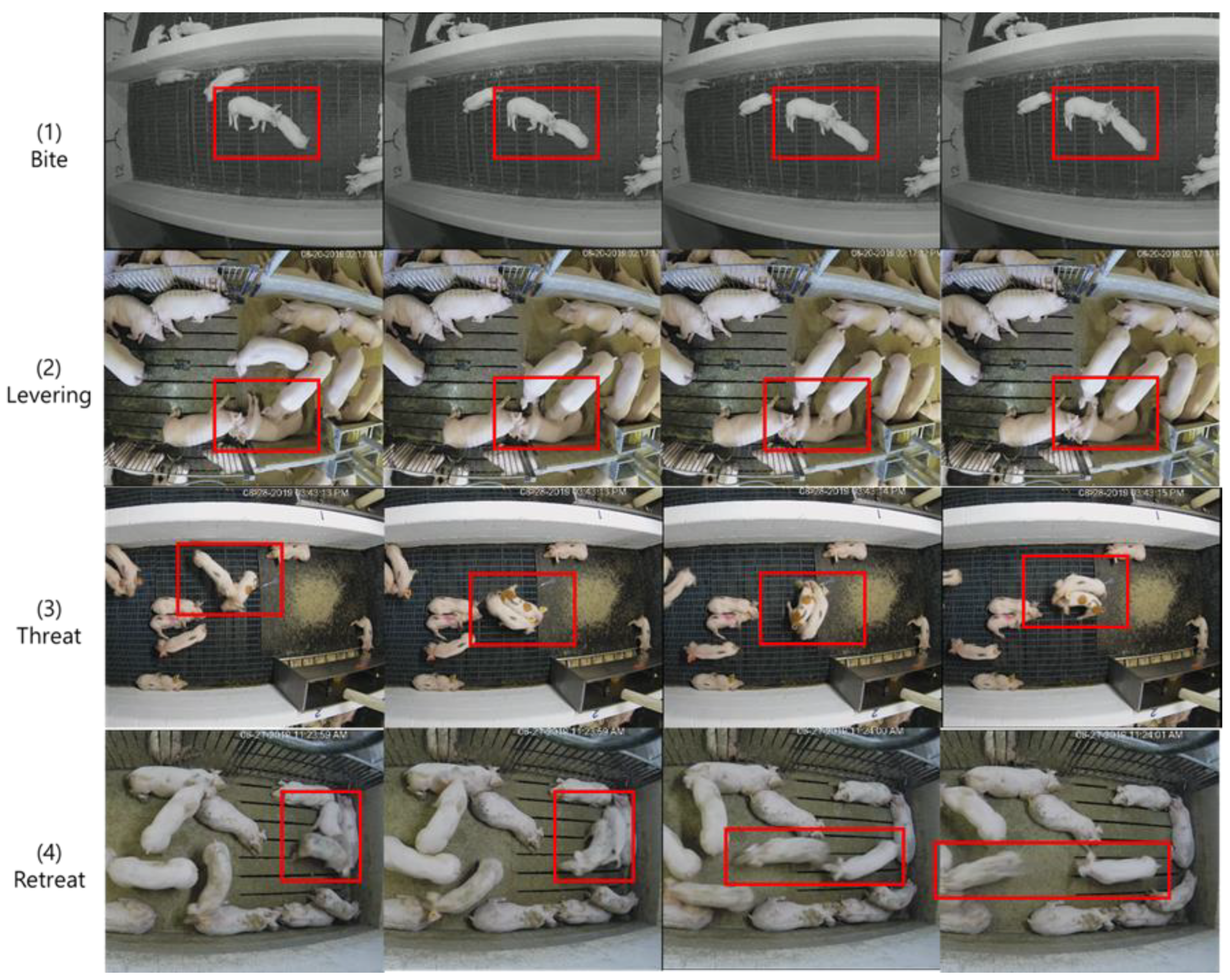
Figure 2.
Workflow of AutoEncoder.
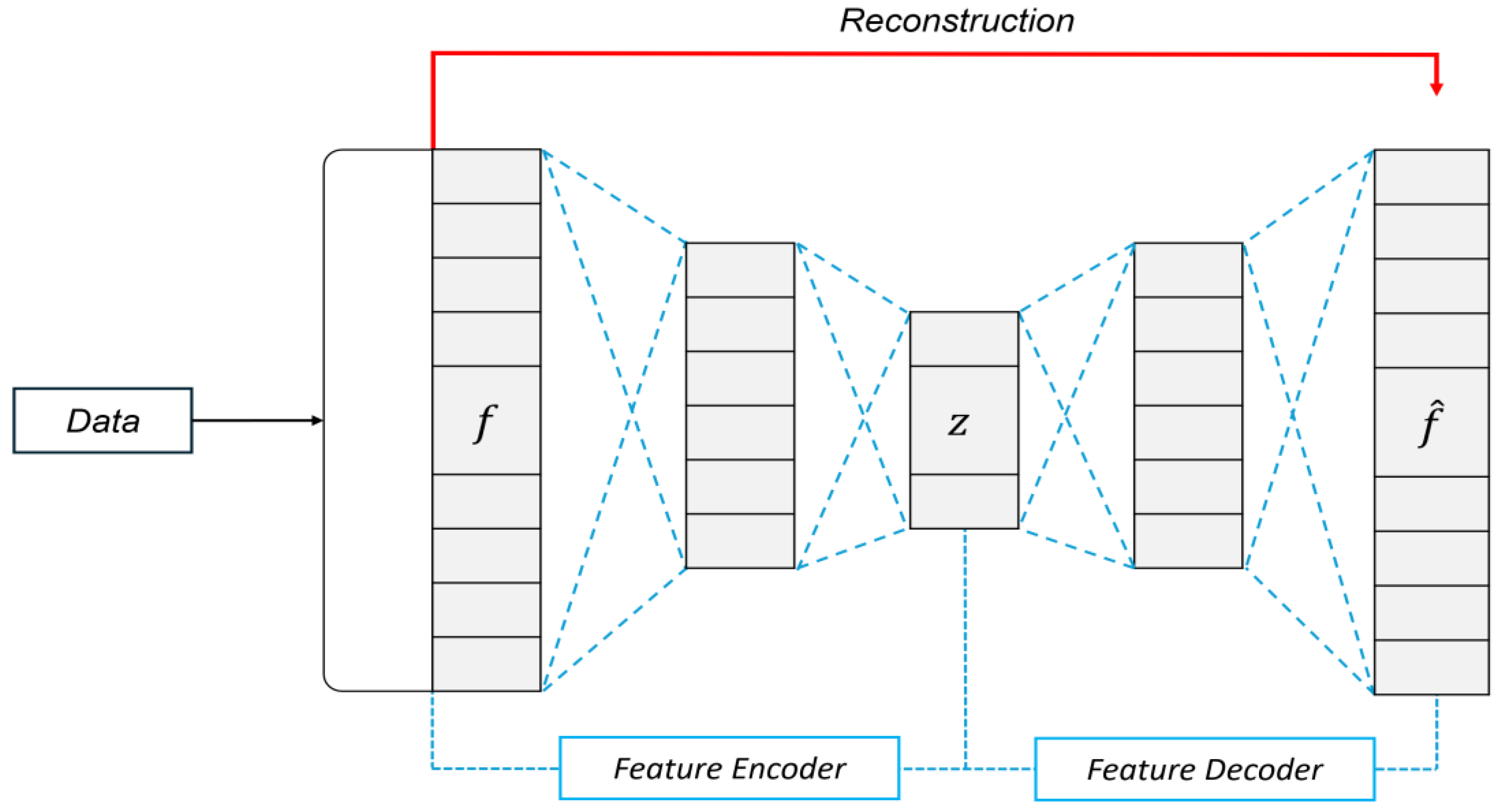
Figure 3.
Workflow of aggression detection.
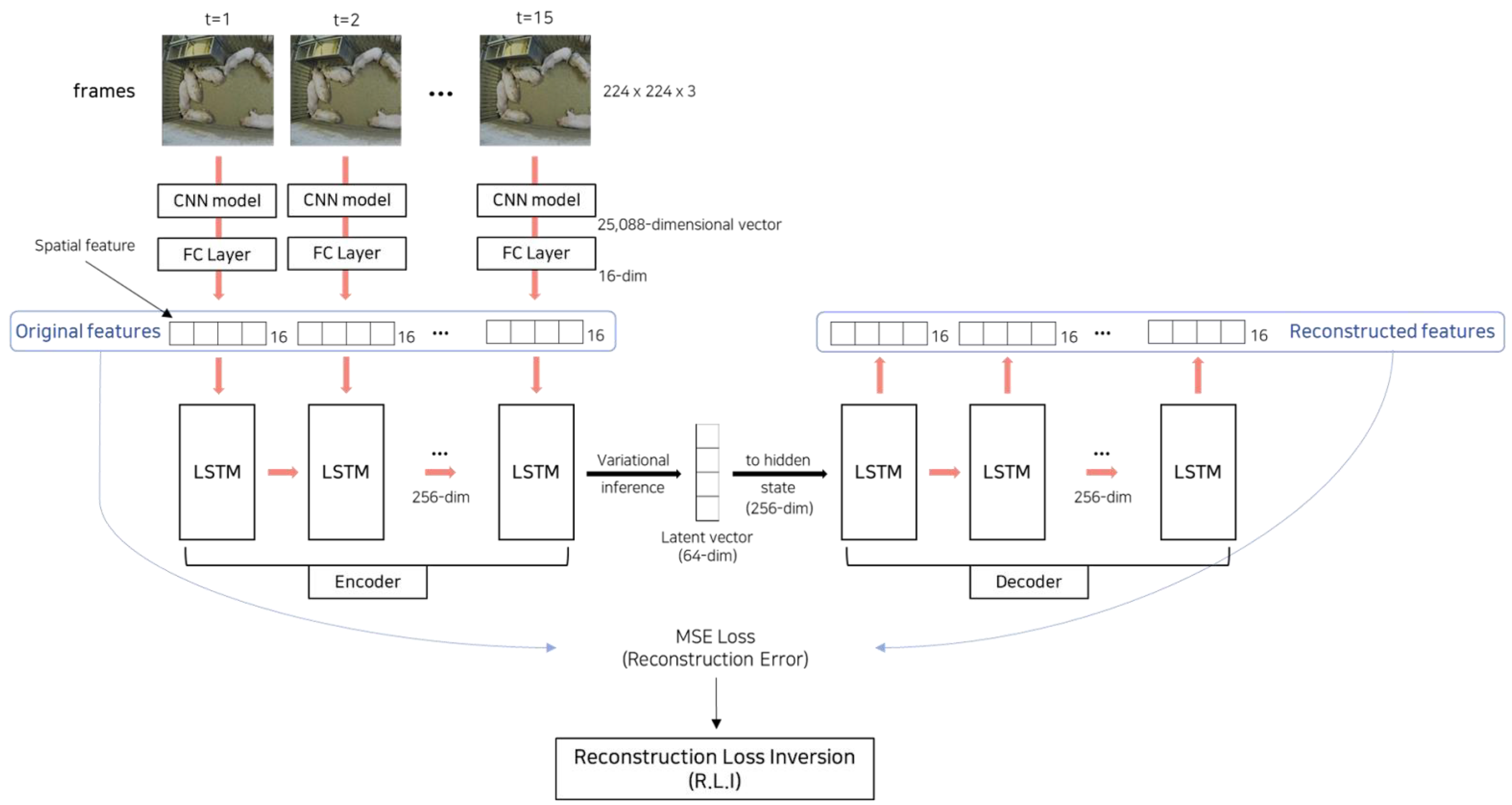
Figure 4.
Distribution of reconstruction error.
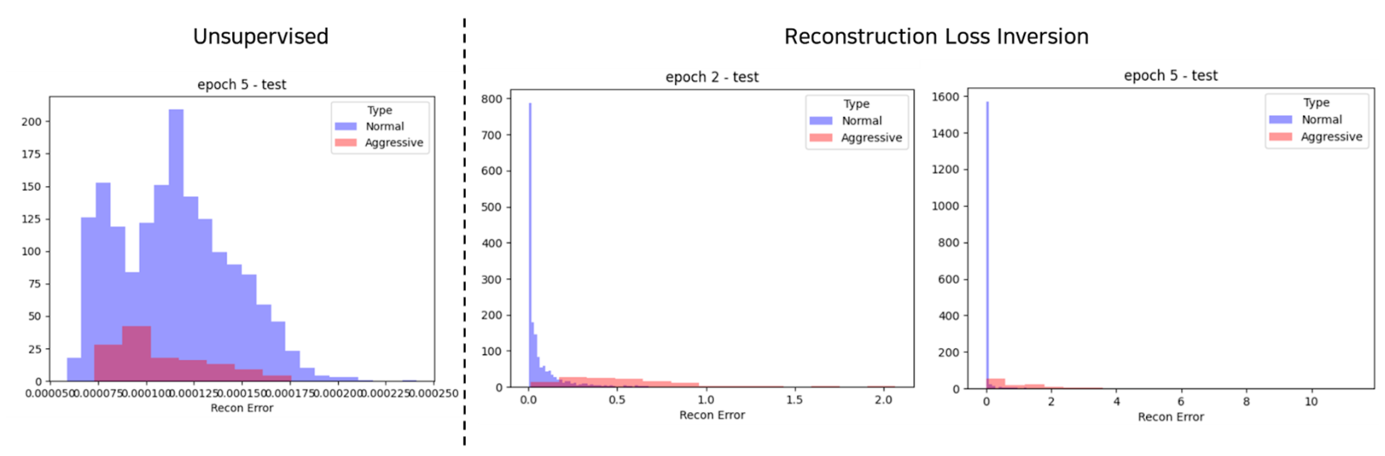
Figure 5.
Distribution of TP, FP, TN, and FN by threshold from the result of Table 6.
Figure 5.
Distribution of TP, FP, TN, and FN by threshold from the result of Table 6.
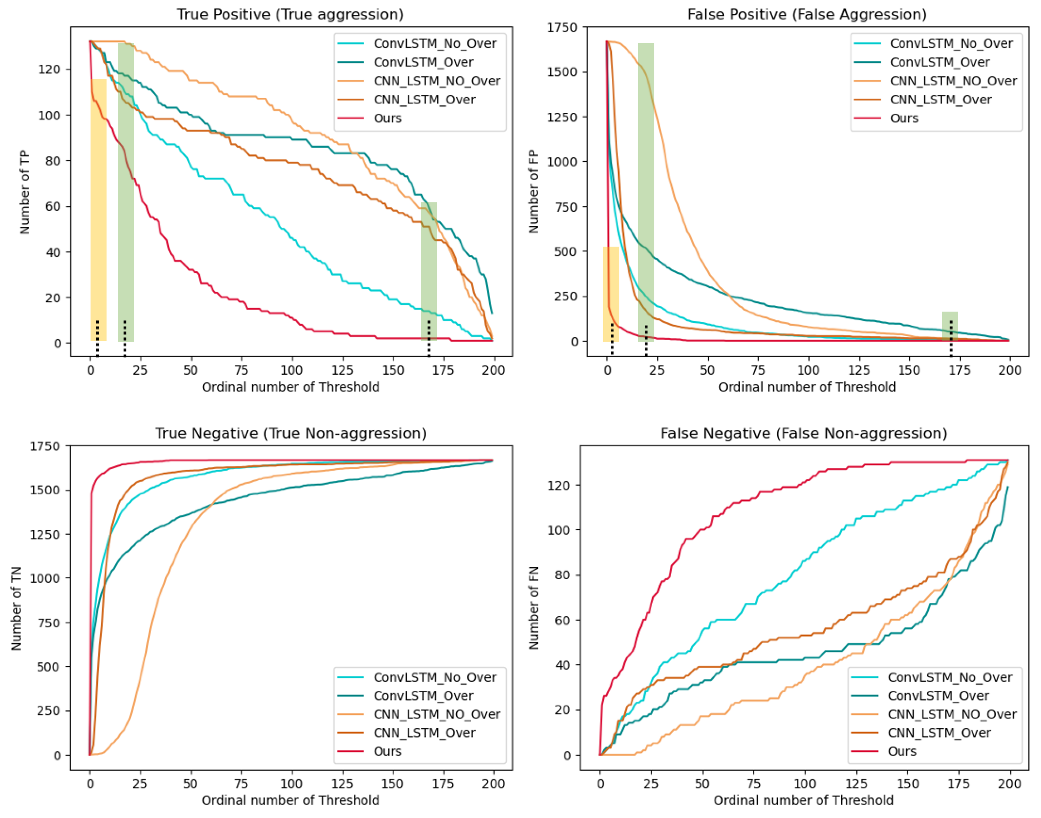

Table 2.
Summary of video data source [15].
Table 2.
Summary of video data source [15].
| Nursery (3~10 weeks) | Early Finisher (11~18 weeks) | Late Finisher (19~26 weeks) | ||||||||||||||
|---|---|---|---|---|---|---|---|---|---|---|---|---|---|---|---|---|
| Video | 1 | 2 | 3 | 4 | 5 | 6 | 7 | 8 | 9 | 10 | 11 | 12 | 13 | 14 | 15 | |
| Day | O | O | O | O | O | O | O | O | O | |||||||
| Night | O | O | O | O | O | O | ||||||||||
| # of the Pigs | 16 | 16 | 15 | 16 | 16 | 7 | 15 | 7 | 8 | 8 | 16 | 14 | 12 | 14 | 13 | |
| Activity Level | H | M | L | M | L | H | M | L | M | L | H | M | L | M | L | |
H: High, M: Medium, L: Low.
Table 2.
Summary of the train set and the test set.
| train | test | ratio | |
|---|---|---|---|
| Non-aggression (0) | 6660 | 1668 | 0.93 |
| Aggression (1) | 531 | 132 | 0.07 |
Table 3.
Optimization for Lambda in Eq (1): l=0.03, 0.05, 0.1, 0.2, 0.4, 0.6, 0.8, 1.0, 2.0.
| Dimension | 16 | 32 | 64 | 128 | 256 | 512 |
|---|---|---|---|---|---|---|
| AUC-ROC | 0.9364 | 0.9382 | 0.9372 | 0.9367 | 0.9373 | 0.9386 |
| AUC-PR | 0.7433 | 0.7296 | 0.7385 | 0.7369 | 0.7324 | 0.7352 |
Table 4.
Optimization for the dimension of a spatial feature: 16, 32, 64, 128, 256, 512.
| Lambda | 0.03 | 0.05 | 0.1 | 0.2 | 0.4 | 0.6 | 0.8 | 1.0 | 2.0 |
|---|---|---|---|---|---|---|---|---|---|
| AUC-ROC | 0.9368 | 0.9367 | 0.9351 | 0.9340 | 0.9327 | 0.9326 | 0.9320 | 0.9336 | 0.9252 |
| AUC-PR | 0.7301 | 0.7369 | 0.7295 | 0.7106 | 0.7120 | 0.6984 | 0.6491 | 0.7050 | 0.6564 |
Table 5.
Optimization for batch size: 2, 4, 6, 8, 10, 12, 14.
| Batch size | 2 | 4 | 6 | 8 | 10 | 12 | 14 |
|---|---|---|---|---|---|---|---|
| AUC-ROC | 0.9274 | 0.9364 | 0.9353 | 0.9349 | 0.9407 | 0.9367 | 0.9409 |
| AUC-PR | 0.6967 | 0.7433 | 0.7343 | 0.7398 | 0.7405 | 0.7387 | 0.7463 |
Table 6.
Model comparison results over classification models. In the table “(over)” means that the experiment was conducted with a dataset with simple oversampling so that the number of aggressive episodes could match the number of non-aggressive episodes in Table 2.
Table 6.
Model comparison results over classification models. In the table “(over)” means that the experiment was conducted with a dataset with simple oversampling so that the number of aggressive episodes could match the number of non-aggressive episodes in Table 2.
| Task | Classification | Anomaly detection | |||
|---|---|---|---|---|---|
| Model | ConvLSTM | ConvLSTM(over) | CNN+LSTM | CNN+LSTM(over) | Ours |
| AUC-ROC | 0.9090 | 0.8954 | 0.9313 | 0.9227 | 0.9409 |
| AUC-PR | 0.5481 | 0.5388 | 0.6965 | 0.6954 | 0.7463 |
Disclaimer/Publisher’s Note: The statements, opinions and data contained in all publications are solely those of the individual author(s) and contributor(s) and not of MDPI and/or the editor(s). MDPI and/or the editor(s) disclaim responsibility for any injury to people or property resulting from any ideas, methods, instructions or products referred to in the content. |
© 2024 by the authors. Licensee MDPI, Basel, Switzerland. This article is an open access article distributed under the terms and conditions of the Creative Commons Attribution (CC BY) license (http://creativecommons.org/licenses/by/4.0/).
Copyright: This open access article is published under a Creative Commons CC BY 4.0 license, which permit the free download, distribution, and reuse, provided that the author and preprint are cited in any reuse.


