
Submitted:
21 August 2024
Posted:
21 August 2024
You are already at the latest version
Abstract
Underwater natural gas pipelines constitute critical infrastructure for energy transportation. Any damage or leakage in these pipelines poses serious security risks, directly threatening marine and lake ecosystems and potentially causing operational issues and economic losses in the energy supply chain. Due to the difficulty in detecting deterioration over time and regularly inspecting these submerged pipelines by divers, the use of unmanned underwater vehicles (UUVs) becomes crucial in this field. In this study, an underwater pipeline tracking experiment was carried out by providing autonomous features to a remote-controlled unmanned underwater vehicle. During the tracking of the underwater pipeline, damages were identified, and the locations of these damages were determined. The navigation information of the underwater vehicle, including orientation in the x, y, z axes (roll, pitch, yaw) from a gyroscope integrated with magnetic compass, speed and position information in the three axes from an accelerometer, and the distance to the water surface from a pressure sensor, was integrated into the vehicle. Pre-tests determined the necessary pulse width modulation values for the thrusters of the vehicle, enabling autonomous operation by providing these values as input to the thruster motors. In this study, the vehicle moves in 3D was achived by the vertical thruster of the vehicle was activated to maintain a specific depth, and applying equal force to the vehicle’s right and left thrusters forward movement, while differential force induced deviation angles. In pool experiments, the unmanned underwater vehicle autonomously tracked the pipeline as intended, identifying damages on the pipeline using images captured by the vehicle's camera. The images for damage assessment were processed using a convolution neural network (CNN) algorithm, which is a deep learning method. The position of the damage relative to the vehicle was estimated from the pixel dimensions of the identified damage. The location of the damage relative to its starting point was obtained by combining these two positional pieces of information from the vehicle's navigation system. The all study was performed within the Python environment.
Keywords:
unmanned underwater vehicle
; convolution neural network
; underwater pipe line tracking
; underwater pipe damage detection
; navigation of unmanned underwater vehicle
1. Introduction
1.1. Motivation
Unmanned underwater observation vehicles are critically important for various military and civilian applications. These unmanned vehicles are used in civilian fields such as underwater mapping, port security, geological geophysics, and fisheries, and in military areas for mine detection, enemy ship detection, ship safety, coastal security, and human detection, as well as in underwater cable and pipeline laying operations [3,4,5]. The highly variable nature of the underwater environment makes these operations challenging. Using unmanned underwater vehicles instead of human divers in long-term operations in dark and deep waters is both safer and more cost-effective due to the potential risks to human life [1,2]. Divers can only remain submerged for a limited time during any underwater operation due to the risk of hypothermia from prolonged exposure. For this reason, the duration of underwater operations tends to be extended. To eliminate the negative aspects arising in similar underwater operations, unmanned underwater vehicles have started to be preferred for underwater tasks.
Underwater natural gas pipelines form a critical infrastructure for energy transportation. Any damage or leakage occurring in these pipelines can create serious security risks. Proper monitoring and damage detection facilitate the early identification and prevention of potential hazards. Additionally, underwater natural gas pipelines can pose a direct threat to marine and lake ecosystems. Any leakage or damage can lead to environmental pollution and harm aquatic life. Timely damage detection can help minimize environmental impacts. Damages to underwater natural gas pipelines can also cause interruptions in the transmission of natural gas, leading to serious operational problems in the energy supply chain. Continuous monitoring and damage detection are crucial for maintaining operational continuity. Furthermore, damages, repairs, and interruptions in the pipeline can lead to significant economic losses for energy companies. Timely damage detection can reduce costly emergency interventions and increase operational efficiency. There are legal and regulatory requirements for underwater natural gas pipelines in many systems. These requirements mandate regular monitoring of the pipelines and the performance of damage detection.
In this study, damages on an underwater pipeline were detected using an unmanned underwater vehicle. As important as detecting damages on the pipeline is knowing the locations of these damages. If the location of the damage is unknown after it has been detected, finding the locations of the damages would require additional time due to the extensive length of the pipelines. In this study, autonomous features were added to the unmanned underwater vehicle, enabling autonomous tracking of the damaged pipeline underwater, and while tracking the pipeline, the damages were diagnosed using artificial learning and their locations were determined.
1.2. Related Studies
For successful execution of unmanned underwater operations, both a well-defined underwater environment and accurate knowledge of the underwater vehicle’s position are necessary [6,7,11],. Therefore, recognizing underwater objects and navigation of underwater vehicles are important. Various types of identification algorithms are available to identify an object. In this study, the convolutional neural network (CNN) training algorithm, a deep learning method, was used. CNNs are used in various fields including image classification, object tracking, object recognition, exposure estimation, text detection and recognition, visual projection detection, action recognition, scene labeling, speech processing, and natural language processing [25]. Other training models require a large amount of prior knowledge at the end of training to achieve high accuracy in object recognition. However, in the CNN model, input data is provided to the model without the need for feature extraction or creation processes. Since the CNN model trains by altering the depth and width of the input image, it determines the features of the image and makes accurate assumptions [10,26]. CNN training is computationally intensive. Various methods have been developed to overcome this problem [27,28,29,30]. The most important of these developments is the development of a CNN model trained using the ImageNet dataset in 2012. This model produced more accurate image classifications than previous methods [26]. He and Zhang in 2018 suggested predicting movements from an image with CNN [31]. Pertusa and Gallego in 2018 used CNN for common object identification on smartphones [32]. In 2015, Li and Shang used the fast region-based CNN (R-CNN) algorithm for underwater fish detection [33]. In 2017, Gomez Chavez and Mueller predicted body posture using the Long Short-Term Memory Recurrent Neural Network (LSTM-RNN) method [34]. The CNN algorithm continues to be used in classification studies today [35,36,37]. Another current machine learning algorithm is the Support Vector Machine (SVM). The SVM algorithm emerged in 1995 [14]. It is a high-performance algorithm frequently chosen for regression and prediction problems [15]. To date, SVM has been used in various contexts including battery life prediction, housing price forecasting, and predicting potential inflation [16,17,18,19]. Although SVM is more commonly chosen for classification problems, Smola and others have shown it can also be used for regression problems [20]. The algorithm used for regression problems is named Support Vector Regression (SVR). SVR has been applied in various regression problems such as motion prediction [22], electric load forecasting [21], and enhancing the performance of filters [12,23,24] . In this study, CNN and SVM were used in a hybrid manner. CNN served as a feature extractor and SVM as a classifier to identify the target object.
Another factor crucial for the successful execution of unmanned underwater operations is the localization of the underwater vehicle [8]. Due to the attenuation/damping of electromagnetic waves underwater, high-accuracy global positioning systems cannot be used. With inertial measurement systems, linear and angular position information is derived from the measured acceleration and angular velocity of the underwater vehicle [9]. Some studies use integrated navigation systems for high accuracy and continuous data transmission. If an INS-GPS integration system is to be used, a surface platform synchronized with the underwater vehicle is essential (referenced in your own publication). In this study, the navigation information of the underwater vehicle was obtained from integrated gyroscopes, magnetic compasses, accelerometers, and pressure sensors.
Despite extensive work on aerial and terrestrial object tracking, there is much less research on underwater object tracking. This is due to the various challenges of working underwater and the degradation of underwater visual data quality, which varies depending on light refraction, water depth, color, and nature. In 2013, Min Li and colleagues presented a method for underwater object identification and tracking based on multi-beam sonar imaging [38]. In 2016, Filip Mandic and colleagues combined sonar and USBL (Ultra Short Baseline) measurements to develop an autonomous surface vehicle and perform underwater object tracking [39]. They developed a filter that combines USBL and sonar image measurements to obtain reliable object tracking predictions even when sonar or USBL measurements are unavailable or erroneous. In addition to object tracking, they focused on adapting only the desired region within the sonar image using the tracking filter’s covariance transformation to improve object identification and filter out erroneous sonar measurements. In 2016, Xianbo Xiang and colleagues proposed a method using magnetic sensing to autonomously track underwater buried cables with a three degrees of freedom (3-DOF) autonomous underwater vehicle [40]. They used feedback linearization technique to design a simplified cable tracking controller based on the geometric relationship between the vehicle and the cable by creating a specialized magnetic line of sight guide. In 2020, Caterina Bigoni and Jan S. Hesthaven suggested a simulation-based decision strategy with machine learning techniques for anomaly detection and damage localization [41]. In 2021, Kakani Katija and colleagues proposed using an underwater vehicle for the visual tracking of deep-sea animals controlled by machine learning [42]. In their study, they presented an integrated tracking algorithm using machine learning that includes multi-class detectors and 3D stereo imaging to track underwater animals over extended periods. There are many studies like these focused on underwater object tracking, and the research continues. Studies such as continuous autonomous tracking and imaging of great white sharks with an autonomous underwater vehicle, and performance analysis of existing underwater object tracking algorithms and dataset creation are available [43,44].
1.3. Contribution
The main contributions of this work are as follows:
- From images experimentally obtained from the integrated camera on the unmanned underwater vehicle, damages on the underwater pipeline were successfully detected using deep learning algorithms.
- The navigation and autopilot of the unmanned underwater vehicle were experimentally performed.
- Autonomous features were added to the remotely operated unmanned underwater vehicle: A series of preliminary tests were conducted to enable the unmanned underwater vehicle to track the underwater pipeline autonomously, independent of remote control. These tests resulted in configuring the necessary input information for the vehicle’s right, left, and vertical thrusters, deriving the relationship between pulse width modulation and linear-angular movements, and setting up the input data required for the vehicle to follow the desired path.
- The experiment of tracking the underwater pipeline with the unmanned underwater vehicle was autonomously and successfully conducted.
- In the underwater pipeline tracking experiment, the locations of the damages on the pipe were detected.
In summary; contrary to some theoretical studies in the literature, autonomous features were added to the unmanned underwater vehicle, allowing it to successfully and autonomously follow the underwater pipeline, and the detection of damages and their locations using a deep learning algorithm was experimentally achieved with success.
1.4. Organization
The paper is organized as follows. The unmanned underwater vehicle used in our underwater experiments is introduced in Section 2. The method used for the underwater pipe damage detection experiment, involving a convolution neural network, and the experimental results of the damage diagnosis are explained in Section 3. The experiment on underwater autonomous pipe tracking and damage location detection is detailed in Section 4. In Section 4, the unmanned underwater vehicle navigation, autopilot, underwater damage location detection, and experimental results are also presented sequentially. In final, the paper is concluded in Section 5.
2. Unmanned Underwater Vehicle
In this study, the remotely operated underwater vehicle (ROV) that will be endowed with autonomous features consists of a user computer, an operator console, and cable section. The unmanned underwater vehicle is equipped with two forward thrusters, one on the left and one on the right, a vertical thruster, and a camera that can rotate 180 degrees. The forward thrusters provide forward movement and yaw orientation, while the vertical thruster provides diving movement. The operator console is used for controlling the vehicle and transferring the data obtained from the vehicle to the computer. The cable ensures data and power transmission between the underwater vehicle and the operator console. In this study, the experimental equipment used in the pool experiment is presented in Figure 1 [48].
The experimental data related to underwater object detection was obtained from a camera integrated into the remotely operated underwater vehicle shown in Figure 1. The camera, with vertical and horizontal fields of view of 128 and 96 degrees respectively and a resolution of 700 TVL, is placed in a waterproof compartment at the front of the vehicle. Weighing approximately 10 kg in air, this vehicle can reach depths of 200 meters to perform tasks such as underwater observation, real-time high-resolution video and photo capture, data collection, and underwater mapping.
3. Underwater Pipe Damage Detection
In this study, damage assessment on the pipeline was conducted using pool images taken from a camera integrated into the unmanned underwater vehicle. The camera, placed in a waterproof compartment at the front of the vehicle, has a vertical field of view of 128 degrees, a horizontal field of view of 96 degrees, and a resolution of 700 TVL [47]. The damage assessment study was carried out in a pool environment based on experimental data. The video footage from the vehicle’s camera was transmitted via fiber optic cable to the operator console and then to a computer via Ethernet cable. To diagnose the damage, the images were processed using a deep learning method, the Convolutional Neural Network (CNN) algorithm. The all study was conducted in a Python environment. The pipes and damages used for the pipeline damage assessment experiment are presented in Figure 2.
3.1. Convolutional Neural Network
3.1.1. İnput Layer
The size of the data provided to this layer is crucial for the success of the model. If the amount of data is too large, the training can yield very successful results but will take a long time. Conversely, if the amount of data is too small, the success rate of the training will significantly decrease.
3.1.2. Convolutional Layer
This layer is the first layer that extracts features from the input data. Different filters are applied to the input data. The applied filters are passed over the entire image to produce an output. The output after applying the filter is known as a feature map [54].
3.1.3. Rectified Linear Unit Layer
The Rectified Linear Unit (ReLU) is a commonly used activation function in CNN [55]. ReLU is defined as follows:
Here, g(y) is a function corresponding to the input y. ReLU sets the negative values of the data applied to its input to zero. This reduces the computational load and training time.
3.1.4. Pooling Layer
The pooling layer is used between successive convolutional layers. The primary purpose of using this layer is to reduce the computational intensity in subsequent layers. There are various pooling methods; one commonly used method is max pooling [56]. In max pooling, the maximum values from the values corresponding to the filter are selected, and the filter moves two steps after each application area.
3.1.5. Fully Connected Layer
A fully connected layer connects to all nodes in all layers before and after it. The fully connected layer adds weights to the data to enable accurate classification of the data received from previous layers. After this process, the network provides predictions. Predictions are obtained by calculating probabilities between feature classes detected in previous layers. If the weighting is incorrect before producing a prediction, the predictions are incorrect and a cost function is calculated. The cost function serves as a guide to optimize our model. The cost function between the actual and predicted networks has been minimized using the backpropagation algorithm [57]. Additionally, overfitting is an undesirable condition in CNNs. The dropout method has been developed in this layer to prevent overfitting [25].
3.1.6. DropOut Layer
In CNNs, excessive training can lead to overfitting—memorization, which reduces the training error at each step during the training of the CNN model, but the test error may not decrease in the same direction. The reliability of a training with overfitting is low, and a training model that starts memorizing is formed. A training model that has overfitted will perform poorly when presented with an image outside of the training dataset. Large datasets like ImageNet have labeled data samples to prevent overfitting [25]. In this study, since the dataset created is not as large as ImageNet, dropout has been used to prevent overfitting.
3.1.7. Classifier Layer
The output value of the classification layer should be equal to the number of objects to be classified. For instance, if five classifications are to be made, the output of the layer should be five. Model predictions are assigned as values in the range of 0–1. A classification can be added to the CNN architecture or created as a separate model. There are different classifier models. In this study, CNN and SVM were used as a hybrid. CNN is a feature extractor, and SVM has been used as a classifier to recognize the object being sought [27]. SVMs choose from an infinite number of decision boundaries that minimize error with the greatest distance between two classes [59]. SVM uses the output of CNN as input and determines the classes by extracting features obtained by CNN. Thus, classification is achieved.
3.2. Convolutional Neural Network Training
To train the CNN architecture, a dataset was created using deep learning and image augmentation methods from photographs of damage taken on the pipeline. For the damage diagnosis study, the dataset from damages on the underwater pipeline was created through data augmentation without altering the characteristic features of the images. The data augmentation methods used for this study include rotating the image horizontally and vertically, rotating the image at specific angles, shifting the image horizontally and vertically, zooming, darkening, lightening, and changing the color. In CNN, each photo collected with the LabelImg program was individually labeled. The labeling process generated files with a .xml extension. After completing the labeling process, the photos were divided into two separate folders to run the training algorithm. These folders are the training and testing folders. Eighty percent of the photos of the object to be detected were placed in the training folder, and twenty percent were placed in the testing folder, and the training of the CNN was initiated.
3.3. Underwater Damage Detection Experiment Results
Using the CNN algorithm, damages on the underwater pipeline in a pool environment were diagnosed online using an unmanned underwater vehicle. The damage diagnosis results are presented in Figure 3. As seen from the figure, high accuracy percentage of pipe damage has been detected with the developed algorithm. Thus, the unmanned underwater vehicle has been endowed with the capability to detect objects through the underwater damage diagnosis test.
In Figure 4, the accuracy and loss curves of the CNN training are visible. The ESA training for damage diagnosis was carried out over 50 epochs. An epoch means that the model sees each data in the dataset once. As seen in Figure 4, both the training loss and the validation/consistency loss have been observed to decrease, which is a desired outcome.
4. Underwater Autonomous Pipe Tracking and Damage Location Detection
In this study, autonomous features were endowed to a remotely operated underwater vehicle, which was then used for underwater pipeline tracking in a pool environment, and damage detection on the pipe as well as the location of this damage were achieved. In the experiment, a schematic representation of the scenario created for the underwater pipeline and images from the pool experiment are given in Figure 5 and Figure 6. As seen in Figure 5, during the experiment, an underwater pipeline was created inside the pool using one 3-meter and two 2-meter pipes.
Preliminary tests were conducted in a pool environment to enable the unmanned underwater vehicle to autonomously follow the desired pipeline. In these tests, the PWM values that need to be applied to the vehicle’s thrusters were determined to enable the vehicle to autonomously perform the following movements: moving forward 3 meters, turning right, moving 2 meters, turning right, and then moving another 2 meters in a linear and angular motions.
In these tests, the vehicle’s speed information corresponding to the PWM values of the thruster motors was obtained by remotely controlling the vehicle to move along different routes. The speed information corresponding to these PWM values and, consequently, the distance information obtained were observed. The necessary PWM values for the vehicle to follow a pipeline of known length, which will be used in the experiment, were determined as a result of these tests and sent to the vehicle’s thruster motors as input information. Consequently, an object tracking algorithm was developed using the data obtained from these preliminary tests to enable the vehicle to autonomously follow the desired object.
During the vehicle’s tracking of the pipeline, the damages on the pipe were detected using the CNN method detailed above. The damage location detection information has been supported with the vehicle navigation and autopilot described in the next section.
4.1. Navigation of Unmanned Underwater Vehicle
The navigation information of unmanned underwater vehicle comes from IMU, depth sensor. IMU with MPU-6000 series used in the experiment combines 3-axis gyroscopes integrated with magnetic compass, 3-axis accelerometer. The depth sensor used in the experiment is the measurement specialties MS5837-30BA, which can measure up to 30 bar (300m/1000 ft depth). In the pool experiments, the speed and orientation information of the unmanned underwater vehicle was obtained from the Inertial Measurement Unit (IMU) sensor integrated into the vehicle. The linear speed of the vehicle used in the pool experiments was obtained by integrating the acceleration. Linear position information was obtained by taking the double integral of the measurement from the accelerometer sensor. The yaw angle (rotation around the z-axis) information was obtained by taking the integral of the gyroscope measurement data once. The depth information of the vehicle from the pool surface was obtained from the pressure sensor integrated into the vehicle [60]. The equations for the vehicle’s linear motion along the x and y axes and angular motion around the z-axis are given in (2), (3) and (4).
4.2. Autopilot of Unmanned Underwater Vehicle
In this study, the Pixhawk control board was used for the autopilot of the unmanned underwater vehicle as seen Figure 7 . Pixhawk is frequently used as a control board for unmanned aerial vehicles, surface, and underwater vehicles due to its low cost and high-performance advantages. In this study, communication between the user computer and the unmanned underwater vehicle, as well as sending inputs to the vehicle via Python software, were carried out using the MAVLink protocol. The pymavlink library was used to establish the connection between the vehicle and Python.
In the experiment, to automate the pipeline tracking, a series of preliminary pool tests were initially conducted to observe the vehicle’s responses to PWM (pulse-width modulation) signals sent to the motors by the Pixhawk. Subsequently, the necessary input value of each thrusters values to be sent to the motors for the created pipeline tracking scenarios were determined. Before the experiment for the established pipeline scenario, the Speed-PWM and Depth-PWM relationships were observed, and the necessary PWM information to enable the vehicle to follow the pipeline was sent to the vehicle.
The vehicle has successfully followed the designated route. The reference and measured forward speed information, yaw angle, and depth information while the vehicle was following the designated pipeline route are shown sequentially in Figures Figure 8, Figure 9, and Figure 10.
Figure 8 shows the necessary reference forward speed information for following the specified pipeline, along with the forward speed information obtained from the accelerometer during the pipeline tracking. Figure 9 presents the necessary yaw angle for the vehicle to follow the specified pipeline in the experiment, along with the yaw angle measured from the gyroscope during the experiment.
4.3. Pipe Line Damage Location Detection
In the pool experiment, while the unmanned underwater vehicle autonomously followed the pipeline as desired, damages on the pipeline were diagnosed using images obtained from the vehicle’s camera. The position of the diagnosed damage relative to the vehicle was estimated from the pixel dimensions of the damage. A dataset was created by calculating pixel values from images of damages taken from different distances. With this dataset, a support vector machine was trained to estimate the distance corresponding to the pixel sizes, and consequently, a model was developed to predict the position of the damage. Additionally, the vehicle’s position at the moment it diagnosed the damage is known from its navigation system. By combining these two pieces of location information, the position of the damage relative to the starting point was determined.
EXPERIMENT RESULTS
For this experiment, one 3-meter and two 2-meter pipes were placed in the pool at 45-degree angles to each other. Prior to the experiment, three separate points on the pipeline positioned in the pool were damaged. These damage images were provided in Section 1, Figure 2. The results of the damage diagnosis with CNN for the pool experiment and the location of this damage are given in Figure 11 to Figure 13.
In Figure 14, the 3D movement of the unmanned underwater vehicle during the autonomous underwater pipeline tracking experiment are presented, respectively. The pipeline that was intended to be followed is shown as a blue line as the reference path, and the path the vehicle actually followed during the experiment is shown as a red line. As can be seen from Figure 14, the vehicle successfully followed the pipeline placed in the pool with high performance.
Figure 10 presents the depth information of the vehicle. In this experiment, the pipeline was placed at a depth of 1.8 meters in the pool. To follow the pipeline from above at this depth, the unmanned underwater vehicle was submerged to a depth of 60 cm in the pool. Figure 9 presents the changes in the yaw angle made by the vehicle while following the pipeline. Initially, the vehicle followed the 3-meter section of the pipeline at a 90-degree deviation angle in about 22 seconds (including 6 seconds of submersion time), the 2-meter section at a 45-degree angle in 10 seconds, and the final 2-meter section again at a 90-degree angle in 10 seconds.
Table 1 presents the root mean square error (RMSE) values for the study of underwater pipeline tracking with an autonomous unmanned underwater observation vehicle. It is the difference between the reference position value and the tracked position value. These RMSE values are known to the user as the path where the pipeline was placed, and were obtained from the path information recorded by the vehicle after completing the pipeline tracking.
5. Conclusions
In this study, a remotely operated unmanned underwater vehicle was endowed with autonomous features and successfully tracked an experimentally placed underwater pipeline. While tracking the pipeline, the vehicle obtained angular position information from the integrated gyroscope, linear speed and position information from the integrated accelerometer, and depth information from the pressure sensor. Damages on the pipeline were successfully identified using a deep learning algorithm, CNN, with underwater images captured by a camera placed in the water-tight compartment of the vehicle. The location of the detected damaged areas was identified as the vehicle followed the pipeline. The entire study was conducted in a Python environment using experimental data. The success of underwater pipeline damage detection was observed to vary depending on factors such as light refraction, water depth, color, and nature. The results obtained in this study demonstrate that detection of deterioration in underwater pipelines and their regular monitoring can be autonomously, safely, and continuously performed using unmanned underwater vehicles.
Author Contributions
Writing, Data curation, Formal analysis, Investigation, Methodology, Visualization, Seda Karadeniz Kartal; Software, Research, Data curation, Recep Fatih Cantekin
Funding
This work is supported by the Scientific and Technological Research Council of Turkey (grant 119E037) and grant 2210-C
Institutional Review Board Statement
Not applicable
Informed Consent Statement
Not applicable
Data Availability Statement
Not applicable
Acknowledgments
This work is supported by the Scientific and Technological Research Council of Turkey (grant 119E037) and 2210-C. The authors are grateful for the support of the Scientific and Technological Research Council of Turkey and project of 119E037 team members and Berna Erol, Ş. Hakan Kutoğlu , M. Kemal Leblebicioğlu, Rıfat Hacıoğlu, K. Sedar Görmüş.
Conflicts of Interest
The authors declare no conflict of interest.
References
- Wynn, Russell B. Autonomous Underwater Vehicles (AUVs): Their Past, Present and Future Contributions to the Advancement of Marine Geoscience. Marine Geology, 352, pp. 451-68, 2014. [CrossRef]
- Dinc M., Chingiz H. Autonomous Underwater Vehicles. Journal of Marine Engineering & Technology, 14(1), pp. 32-43, 2015. [CrossRef]
- Alvarez, A. Redesigning the SLOCUM Glider for Torpedo Tube Launching. IEEE Journal of Oceanic Engineering 35(4), pp. 984-91 pp, 2010. [CrossRef]
- Bishop, G.C. Gravitational Field Maps And Navigational Errors. Proceedings of the 2000 International Symposium on Underwater Technology, pp. 149-54 pp, 2000. [CrossRef]
- Fattah S. A., Abedin F. R3Diver: Remote Robotic Rescue Diver For Rapid Underwater Search And Rescue Operation. 2016 IEEE Region 10 Conference (TENCON), pp, 3280-83, 2016. [CrossRef]
- Lee, J., Park, J.-H., Hwang, J.-H., Noh, K., Choi, Y., Suh, J. Artificial Neural Network for Glider Detection in a Marine Environment by Improving a CNN Vision Encoder. J. Mar. Sci. Eng., v(12), pp.1106, 2024. [CrossRef]
- Xia, T., Cui, D., Chu, Z., Yu, X. Autonomous Heading Planning and Control Method of Unmanned Underwater Vehicles for Tunnel Detection. J. Mar. Sci. Eng., v(11), pp.740, 2023. [CrossRef]
- Liang, Z., Wang, K., Zhang, J., Zhang, F. An Underwater Multisensor Fusion Simultaneous Localization and Mapping System Based on Image Enhancement. J. Mar. Sci. Eng., v(12), pp.1170, 2024. [CrossRef]
- Wang, C., Cheng, C., Cao, C., Guo, X., Pan, G., Zhang, F. An Invariant Filtering Method Based on Frame Transformed for Underwater INS/DVL/PS Navigation. J. Mar. Sci. Eng., v(12), pp.1178, 2024. [CrossRef]
- Kaya Ustabaş G., Kocabaş S., Kartal S., Kaya H., Tekin I. Ö., Tığlı Aydin R.S., Kutoğlu Ş. H. Detection of airborne nanoparticles with lateral shearing digital holographic microscopy. Optics and Lasers in Engineering, v(151),pp.106934, 2022. [CrossRef]
- Kartal, S.K., Hacıoğlu R., Görmüş S. K.,Kutoğlu, Ş.H., Leblebicioğlu, M.K. Modeling and Analysis of Sea-Surface Vehicle System for Underwater Mapping Using Single-Beam Echosounder. J. Mar. Sci. Eng., v(10), pp.1349, 2022. [CrossRef]
- Erol, B.; Cantekin, R.; Kartal, S.K.; Hacioglu, R.; Gormus, S.; Kutoglu, H.; Leblebicioglu, K. Estimation of Unmanned Underwater Vehicle Motion with Kalman Filter and Improvement by Machine Learning. Int. J. Adv. Eng. Pure Sci. 2021, 33, 67–77. [Google Scholar]
- Solomatine D. P., Shrestha D. L. A novel method to estimate model uncertainty using machine learning techniques. Water Resources Research, 45(12), pp. 1–16 pp, 2009. [CrossRef]
- Cortes C., Vapnik V. Support-Vector Networks Machine Learning. Springer, 20, pp. 273-297, 1995. [CrossRef]
- Zhang Z., Ding S. MBSVR: Multiple birth support vector regressions. Information Sciences. 552, pp. 65-79, 2021. [CrossRef]
- Zhao Q., Qin X. A novel prediction method based on the support vector regression for the remaining useful life of lithium-ion batteries. Microelectronics Reliability, 85, pp. 99-108, 2018. [CrossRef]
- Li X., Shu X. An On-Board Remaining Useful Life Estimation Algorithm for Lithium-Ion Batteries of Electric Vehicles. Energies, 10(5), pp. 691, 2017. [CrossRef]
- Oktanisa I., Mahmudy W. F. Inflation Rate Prediction in Indonesia using Optimized Support Vector Regression Model. Journal of Information Technology and Computer Science, 5(1): pp. 104-114, 2020. [CrossRef]
- Manasa J., Grupta R. Machine Learning based Predicting House Prices using Regression Techniques. 2nd International Conference on Innovative Mechanisms for Industry Applications, (ICIMIA), pp. 624-630, 2020. [CrossRef]
- Smola A. J., Schölkopf B. A Tutorial On Support Vector Regression. Statistics and Computing, 14(3): pp. 199-222, 2004. [CrossRef]
- Dong Y., Zhang Z. A Hybrid Seasonal Mechanism With A Chaotic Cuckoo Search Algorithm With A Support Vector Regression Model For Electric Load Forecasting. Energies, MDPI, 11(4): pp. 1-21, 2018. [CrossRef]
- Li M. W., Geng J. Periodogram Estimation Based On LSSVR-CCPSO Compensation For Forecasting Ship Motion. Nonlinear Dynamics, 97 (4): pp. 2579-2594, 2019. [CrossRef]
- Cheng K., Lu Z. Active Learning Bayesian Support Vector Regression Model For Global Approximation. Information Sciences, 544: pp. 549-563 pp, 2021. [CrossRef]
- Zhang Z., Ding S. A Support Vector Regression Model Hybridized With Chaotic Krill Herd Algorithm And Empirical Mode Decomposition For Regression Task. Neurocomputing. 410: pp. 185-201, 2020. [CrossRef]
- Gu J., Wang Z. Recent Advances İn Convolutional Neural Networks. Pattern Recognition, 77: pp. 354-77, 2018. [CrossRef]
- Gu J., Wang Z. Recent Advances İn Convolutional Neural Networks. Pattern Recognition, 77: pp. 354-77, 2018. [CrossRef]
- Niu X., Ching Y. S. A Novel Hybrid CNN-SVM Classifier For Recognizing Handwritten Digits | Pattern Recognition. Pattern Recognition, 45(4): pp. 131825, 2011. [CrossRef]
- Russakovsky O., Deng J. ImageNet Large Scale Visual Recognition Challenge. International Journal of Computer Vision, 115(3): pp. 211-52, 2015. [CrossRef]
- Simonyan K., Andrew Z. Very Deep Convolutional Networks for Large-Scale Image Recognition. arXiv:1409.1556 [cs]. pp. 1-14, 2015.
- Szegedy C., Liu W. Going Deeper With Convolutions. IEEE Conference on Computer Vision and Pattern Recognition (CVPR), pp.1-9, 2015.
- He X., Wei Z. Emotion Recognition By Assisted Learning With Convolutional Neural Networks. Neurocomputing, 291: pp.187-94, 2018. [CrossRef]
- Pertusa A., Gallego A. MirBot: A Collaborative Object Recognition System for Smartphones Using Convolutional Neural Networks. Neurocomputing, 293: pp.87-99, 2018. [CrossRef]
- Li X., Min S. Fast Accurate Fish Detection And Recognition Of Underwater İmages With Fast R-CNN. OCEANS MTS/IEEE Washington, 2015. [CrossRef]
- Chavez A. G., Birk A. Stereo-Vision Based Diver Pose Estimation Using LSTM Recurrent Neural Networks For AUV Navigation Guidance. OCEANS-Aberdeen, pp.1-7 pp, 2017. [CrossRef]
- Buß, M., Steiniger, Y. Hand-Crafted Feature Based Classification against Convolutional Neural Networks for False Alarm Reduction on Active Diver Detection Sonar Data. OCEANS MTS/IEEE Charleston, pp.1-7, 2018. [CrossRef]
- Williams D. P. Demystifying Deep Convolutional Neural Networks For Sonar Image Classification. NATO STO Centre for Maritime Research and Experimentation (CMRE) Viale San Bartolomeo, 400: pp.513-520, 2019.
- Williams D. P. On the Use of Tiny Convolutional Neural Networks for Human-Expert-Level Classification Performance in Sonar Imagery. IEEE Journal of Oceanic Engineering, 46(1), pp.236-260, 2020. [CrossRef]
- Li M., Ji H. Underwater Object Detection And Tracking Based On Multi-Beam Sonar İmage Processing. IEEE International Conference on Robotics and Biomimetics (ROBIO), pp.1071-76, 2013. [CrossRef]
- Mandic F., Ivor R. Underwater Object Tracking Using Sonar and USBL Measurements. Journal of Sensors, 2016. [CrossRef]
- Xiang X., Caoyang Y. Autonomous Underwater Vehicle with Magnetic Sensing Guidance. Sensors, MDPI, 16(8): pp.1335, 2016. [CrossRef]
- Bigoni C., Hesthaven J. Simulation-Based Anomaly Detection and Damage Localization: An Application to Structural Health Monitoring. Computer Methods in Applied Mechanics and Engineering, 363: pp.112896, 2020. [CrossRef]
- Katija K., Roberts P. Visual Tracking Of Deepwater Animals Using Machine Learning-Controlled Robotic Underwater Vehicles. IEEE Winter Conference on Applications of Computer Vision (WACV), pp.859-68, 2021. [CrossRef]
- Packard G. E., Kukulya A. Continuous Autonomous Tracking And İmaging Of White Sharks And Basking Sharks Using a REMUS-100 AUV. OCEANS, pp.1-5 pp, 2013.
- Kezebou L., Oludare V. Underwater Object Tracking Benchmark and Dataset. IEEE International Symposium on Technologies for Homeland Security (HST), pp.1-6 pp, 2019. [CrossRef]
- Fossen T. I., Guidance and Control of Ocean Vehicles, Wiley, 1999.
- The Nature of Statistical Learning Theory. Springer, New York, 2000.
- Kartal S., Leblebicioğlu M. K. Experimental Test of the Acoustic-Based Navigation and System Detection of an Unmanned Underwater Survey Vehicle (SAGA). Transactions of the Institute of Measurement and Control, 40(8): pp.247-687, 2018.
- Kartal S., Leblebicioğlu M. K. Experimental test of vision-based navigation and system identification of an unmanned underwater survey vehicle (SAGA) for the yaw motion. Transactions of the Institute of Measurement and Control, 41(8):2160-2170, 2019. [CrossRef]
- Perlin H. A., Heitor S. L. Extracting Human Attributes Using a Convolutional Neural Network Approach. Pattern Recognition Letters, 68: pp.250-59, 2015. [CrossRef]
- Lecun Y., Bottou L. Gradient-Based Learning Applied to Document Recognition. Proceedings of the IEEE, 86(11), pp.2278-2324, 1998.
- Wang G., Zhang L. Longitudinal Tear Detection of Conveyor Belt under Uneven Light Based on Haar-AdaBoost and Cascade Algorithm. IEEE Access, pp.108-341, 2020. [CrossRef]
- Zeiler M. D., Rob F. Visualizing and Understanding Convolutional Networks. Computer Vision, Springer International Publishing, pp.818-33, 2014. [CrossRef]
- Lecun Y., Yoshua B. Deep Learning. Nature, 521(7553): pp.436-44, 2015. [CrossRef]
- He K., Xiangyu Z. Spatial Pyramid Pooling in Deep Convolutional Networks for Visual Recognition. Computer Vision, Springer International Publishing, v(37), pp.346-61, 2014. [CrossRef]
- Nair V., Geoffrey E. H. Rectified Linear Units Improve Restricted Boltzmann Machines. In Proceedings of the International Conference on Machine Learning, ICML10, Omnipress, v(27), pp.807-814, 2010.
- Albawi S., Tareq A. M. Understanding of a Convolutional Neural Network. In 2017 International Conference on Engineering and Technology (ICET), pp.16-21, 2017.
- Albawi S., Tareq A. M. Artificial Convolution Neural Network for Medical Image Pattern Recognition. Neural Networks, 8(7): pp.1201-14, 1995. [CrossRef]
- Pal M., Giles M. F. Feature Selection for Classification of Hyperspectral Data by SVM. IEEE Transactions on Geoscience and Remote Sensing, 48(5): pp.2297-2307, 2010.
- DE O., Diulhio C. Using Deep Learning and Low-Cost RGB and Thermal Cameras to Detect Pedestrians in Aerial Images Captured by Multirotor UAV. Sensors, 18(7): pp.2244, sensors, MDPI, 2018. [CrossRef]
- Caccia M., Bibuli R. Basic Navigation, Guidance And Control Of An Unmanned Surface Vehicle. Auton. Robots, v(25), pp.349-365, 2008. [CrossRef]
- Kumar P., Supraja B. et al. Real-Time Concrete Damage Detection Using Deep Learning for High Rise Structures. IEEE Access, 9: pp.112312-31, 2021. [CrossRef]
- Edge C., Enan S. et al. Design and Experiments with LoCO AUV. IEEE/RSJ International Conference on Intelligent Robots and Systems, IROS 2020, pp.1761-68, 2020. [CrossRef]
- Manzanlilla A., Sanchez S. et al. Autonomous Navigation for Unmanned Underwater Vehicles: Real-Time Experiments Using Computer Vision. IEEE Robotics and Automation Letters, 4(2): pp, 1351-56, 2019. [CrossRef]
- Yu Z., Zhang Y. et al. Distributed Adaptive Fault-Tolerant Time-Varying Formation Control of Unmanned Airships With Limited Communication Ranges Against Input Saturation for Smart City Observation. IEEE transactions on neural networks and learning systems, 33(5): pp.1891-1904, 2022. [CrossRef]
Figure 1.
Unmanned underwater vehicle used in the experiment
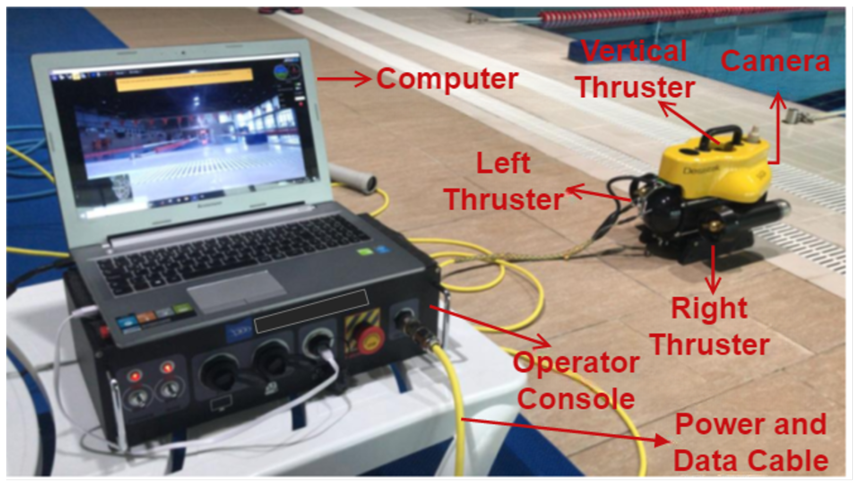
Figure 2.
Damaged pipe used in the experiment
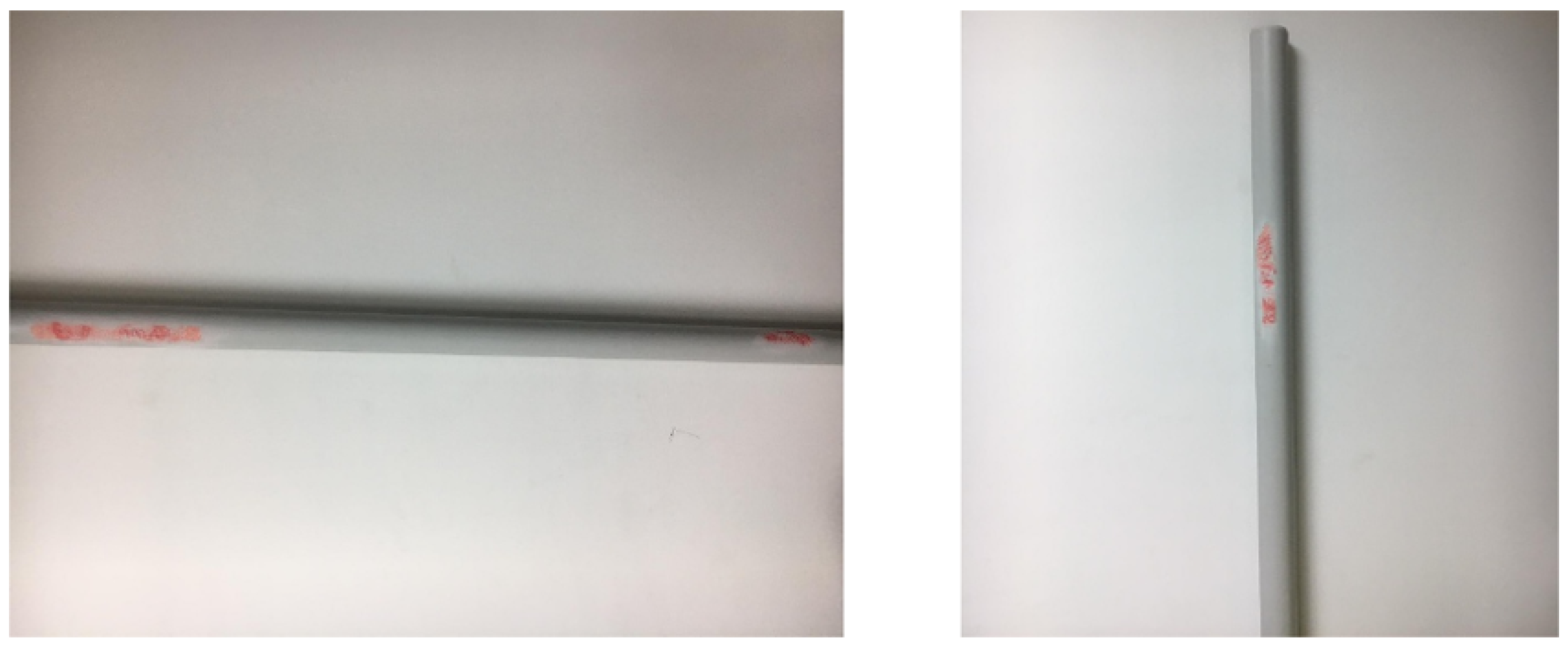
Figure 3.
Damage detection experiment results
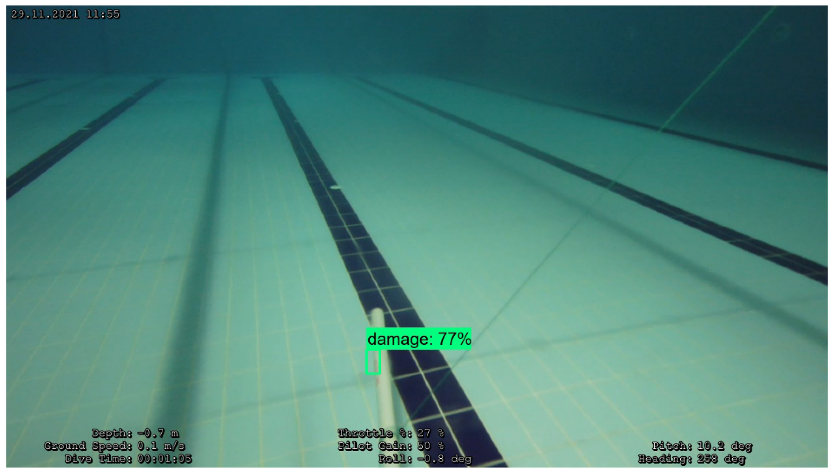
Figure 4.
CNN training consistency and loss curves
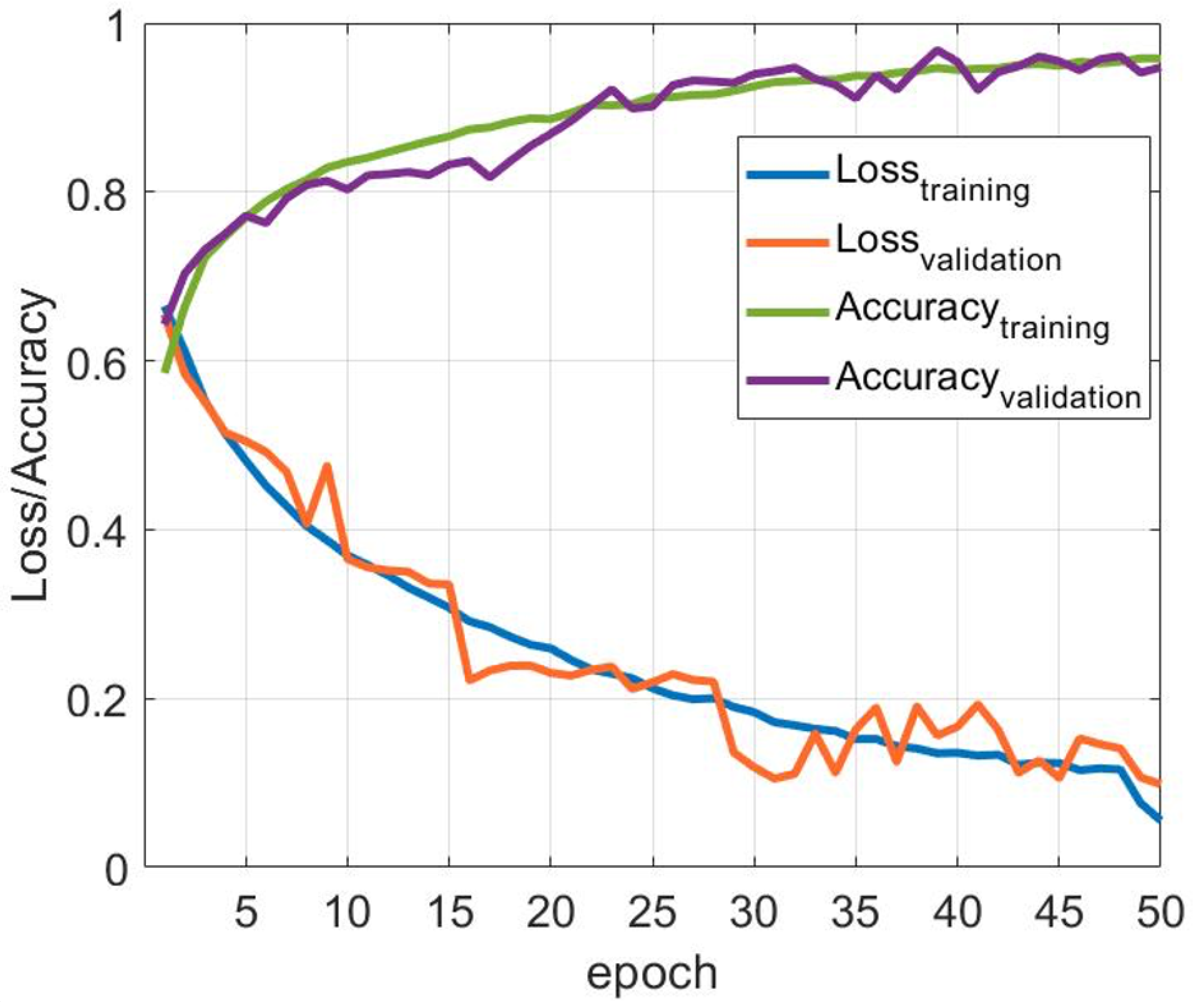
Figure 5.
Pipeline tracking experiment scenario view
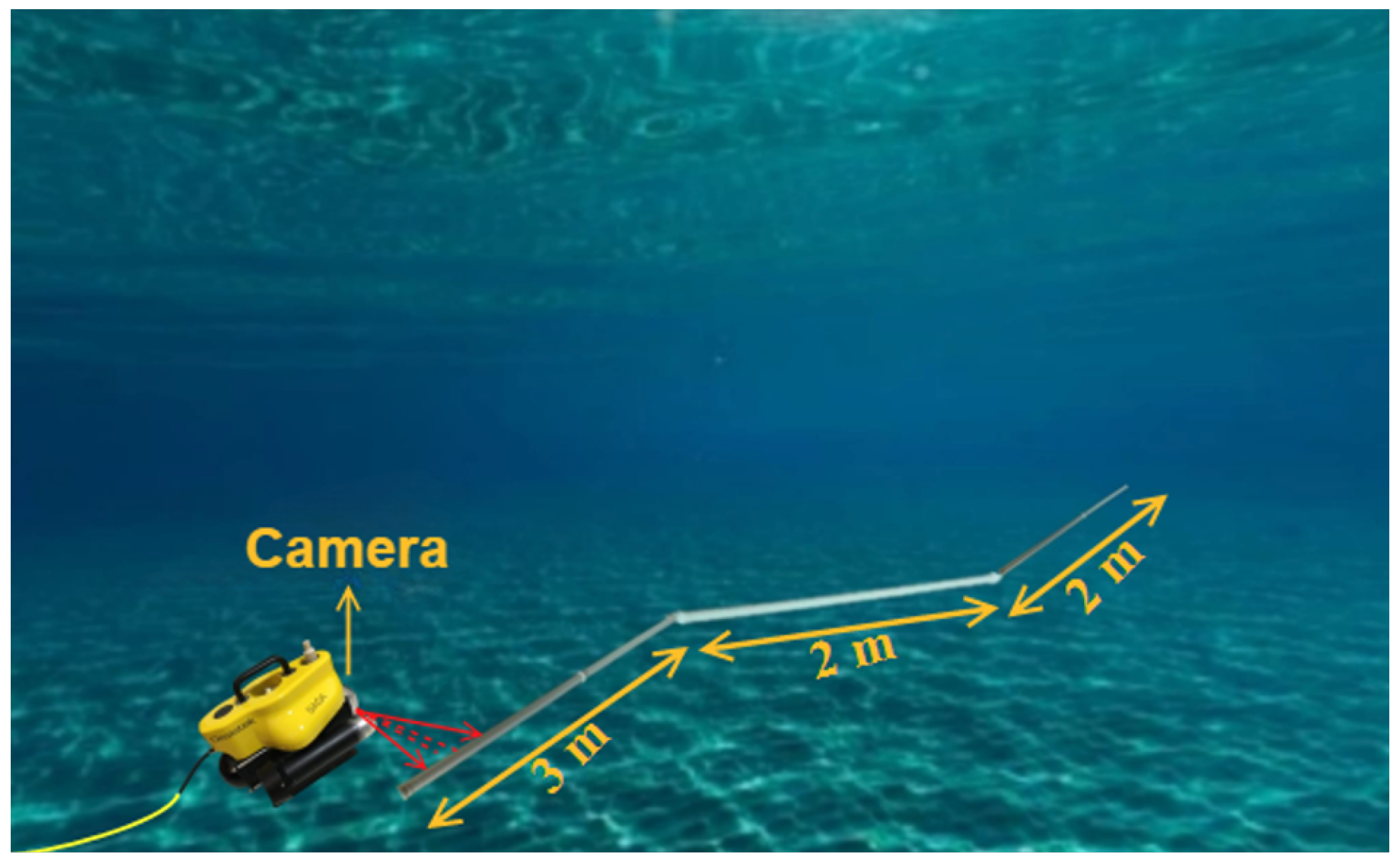
Figure 6.
Pipeline tracking pool experiment
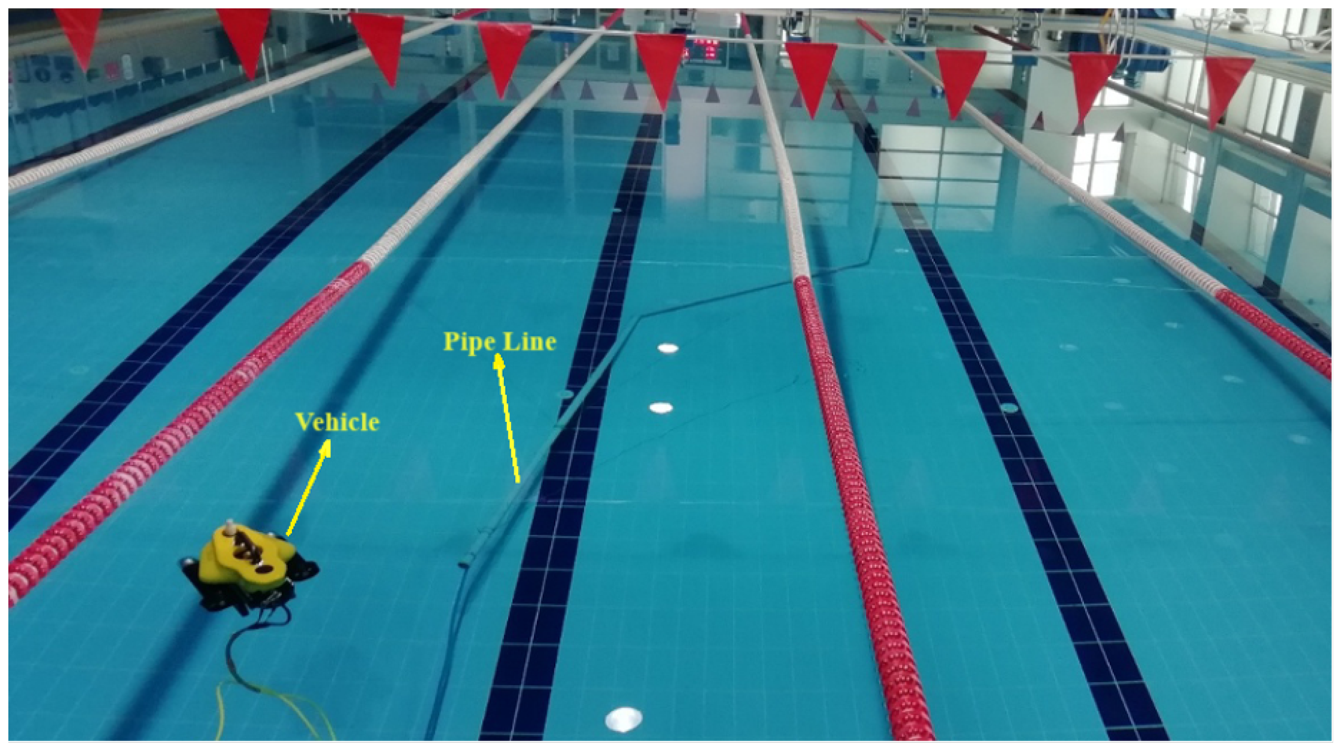
Figure 7.
Vehicle’s pixhawk and thrusters used in the experiment
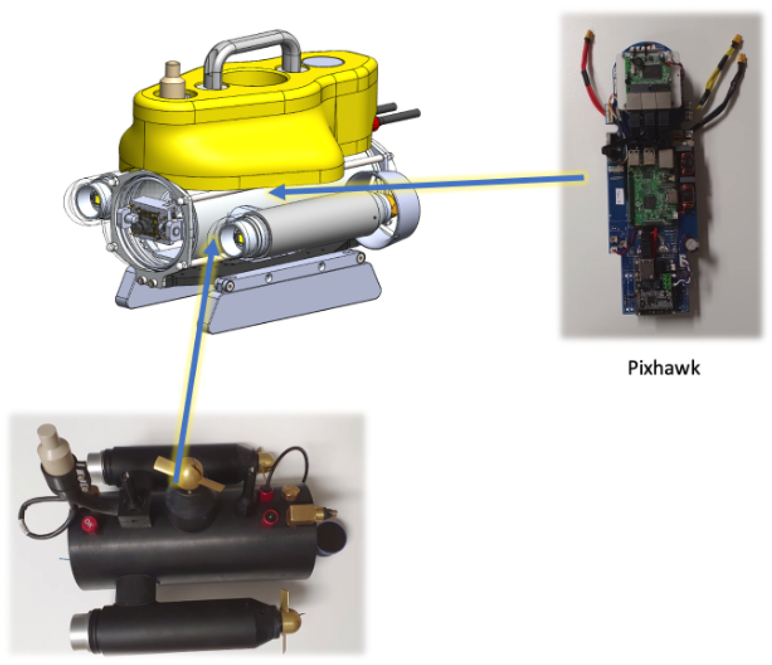
Figure 8.
Reference surge speed (blue line) and measured (red line) surge speed
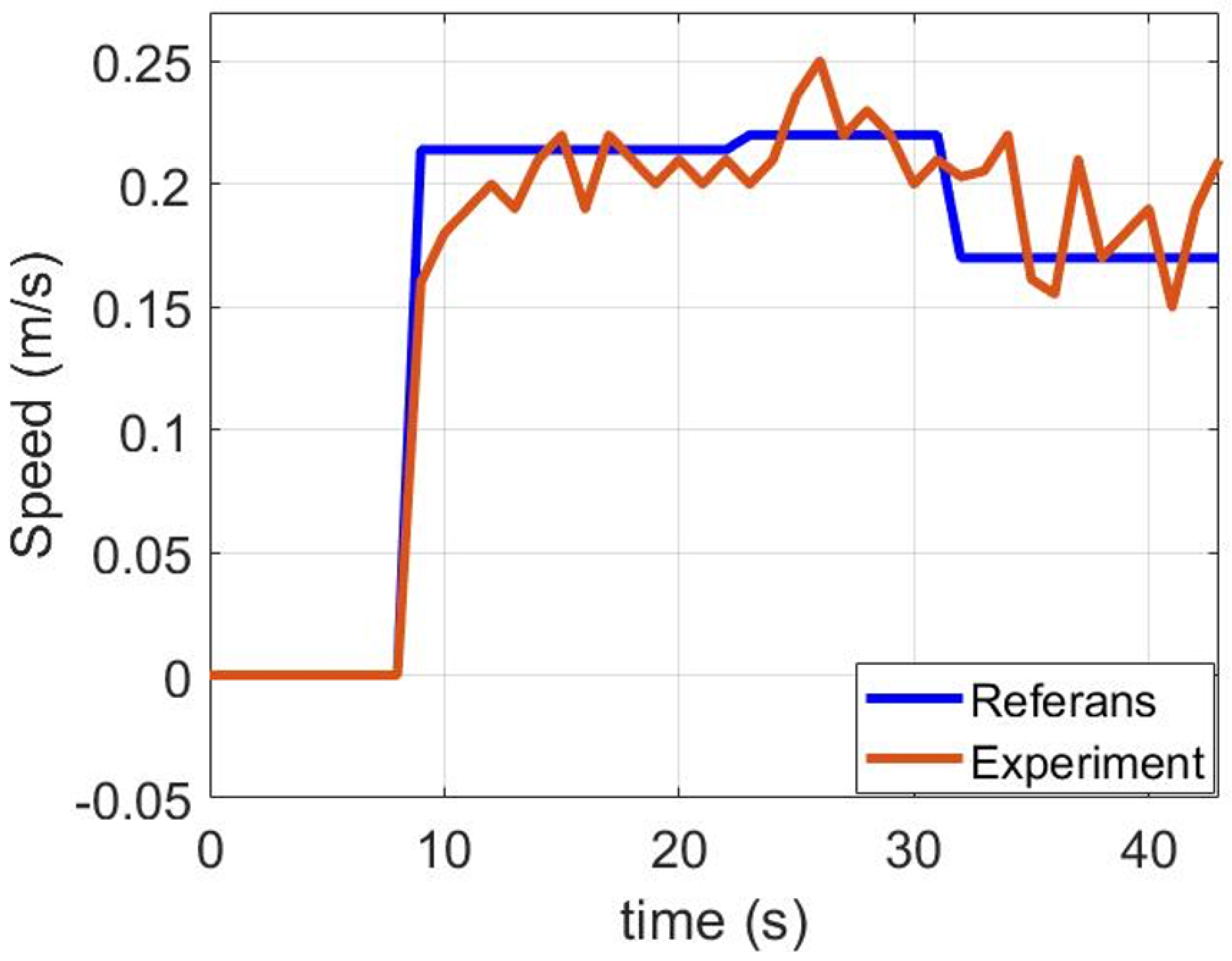
Figure 9.
Reference yaw angle (blue line) and measured yaw angle (red line)
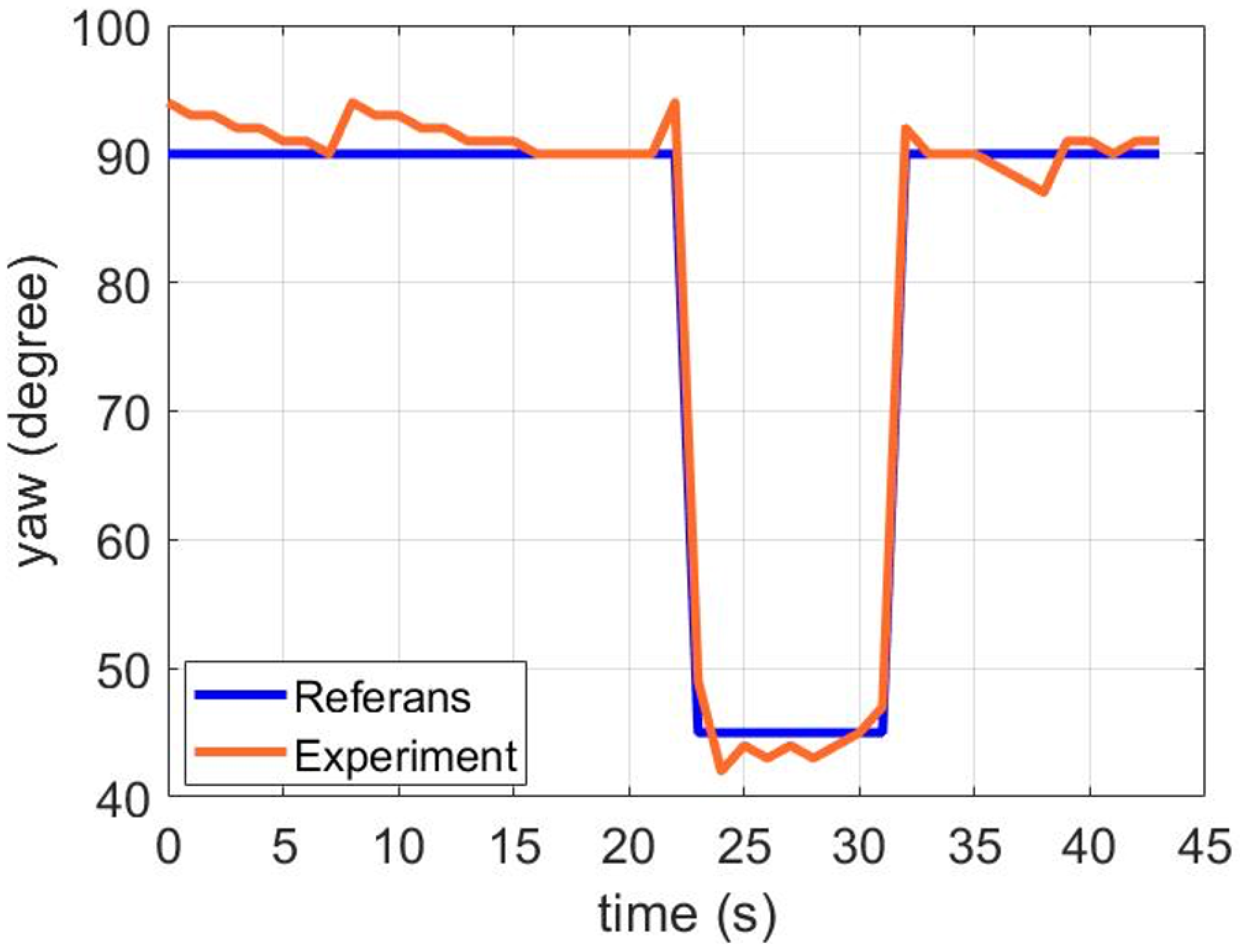
Figure 10.
Reference depth value (blue line) and measured depth value (red line)
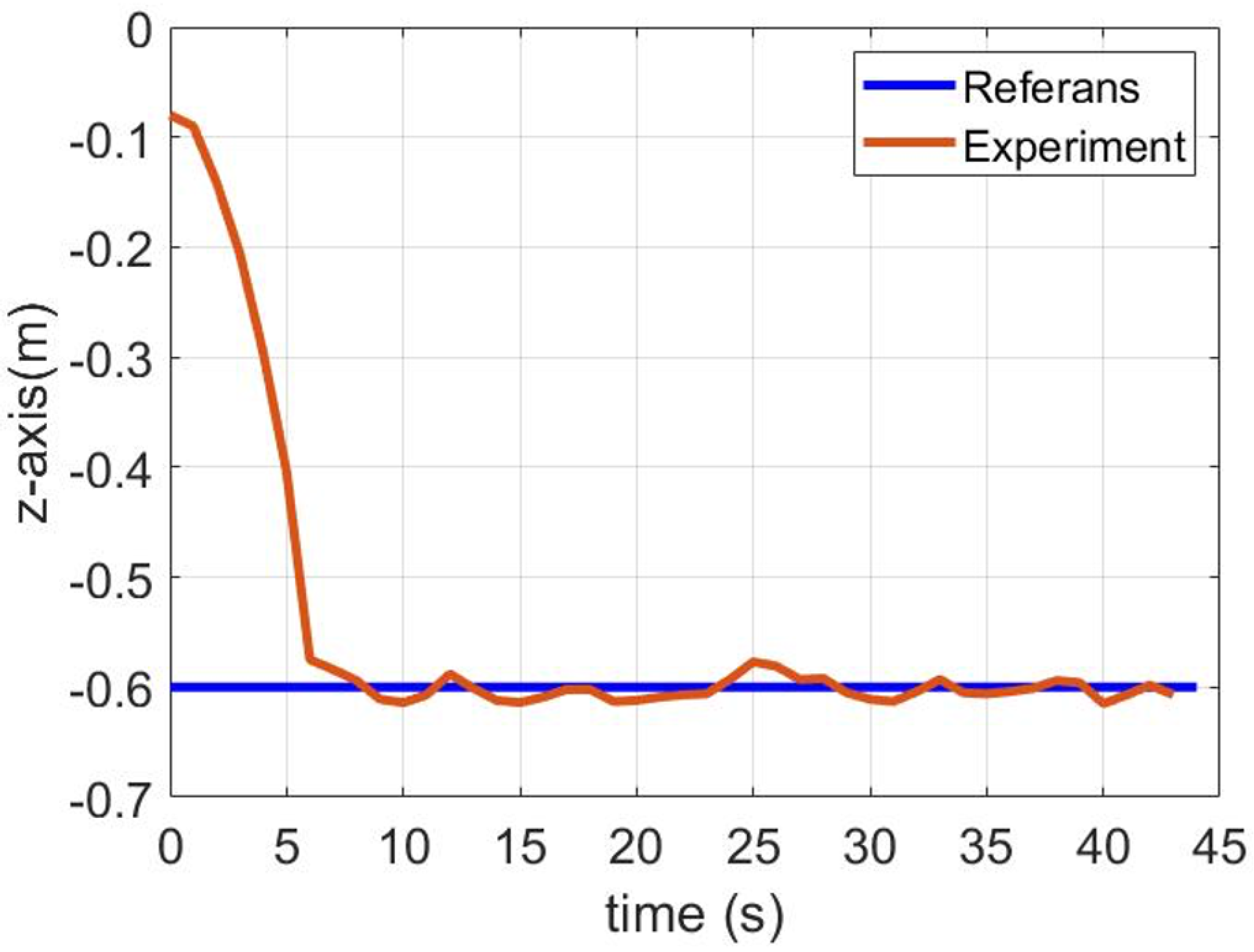
Figure 11.
Location 1 of pipe line damage detection
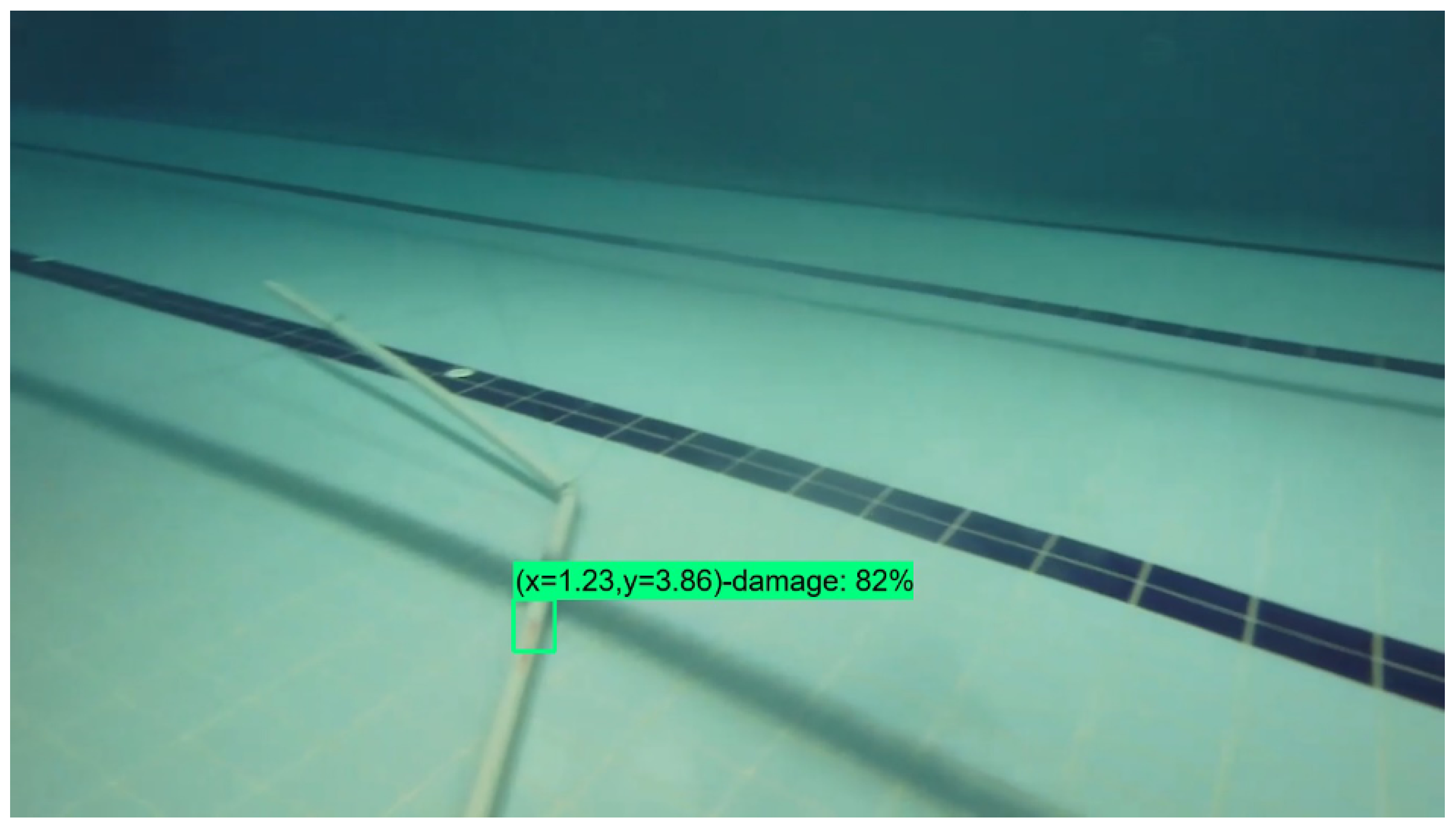
Figure 12.
Location 2 of pipe line damage detection
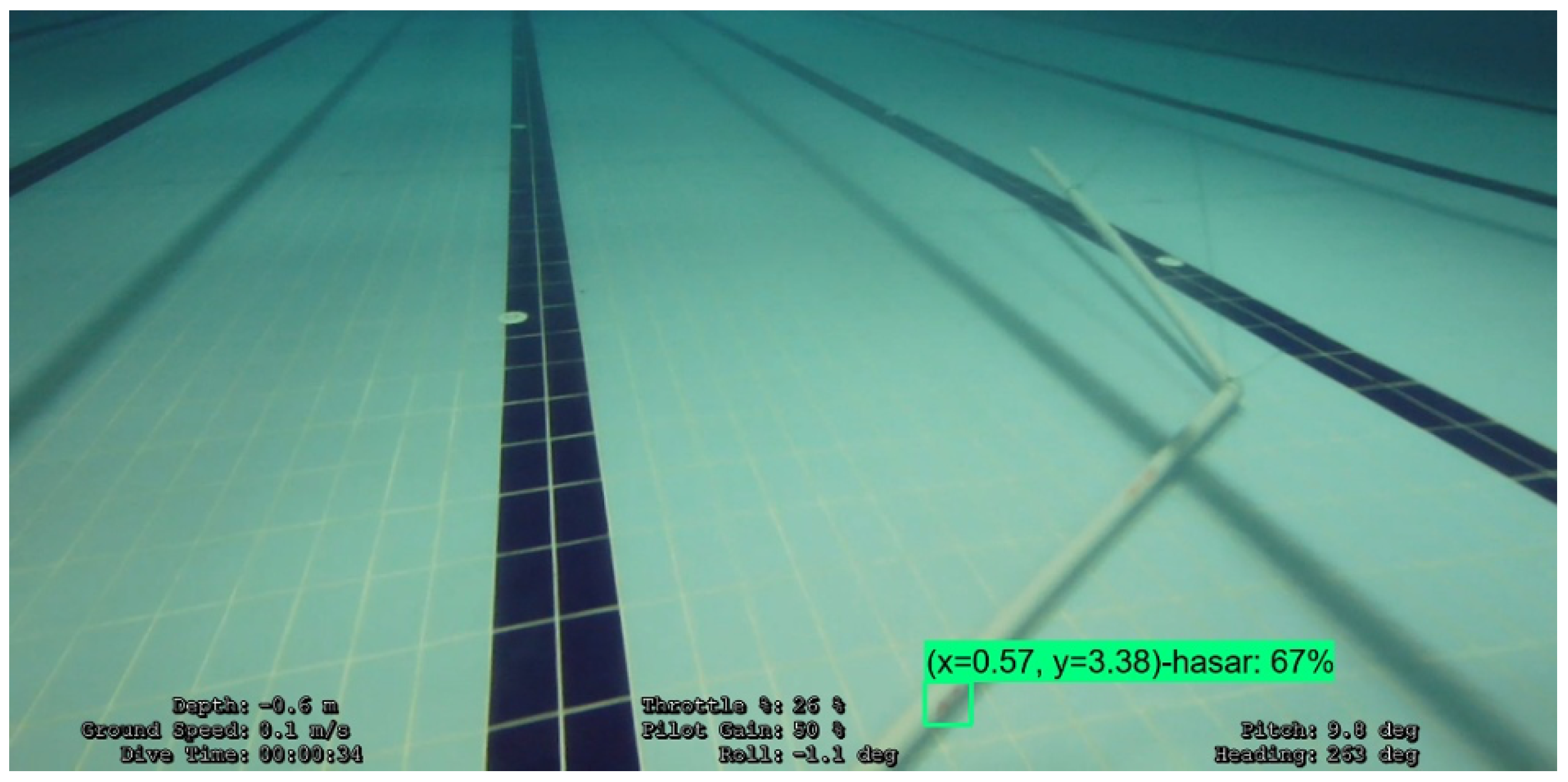
Figure 13.
Location 3 of pipe line damage detection
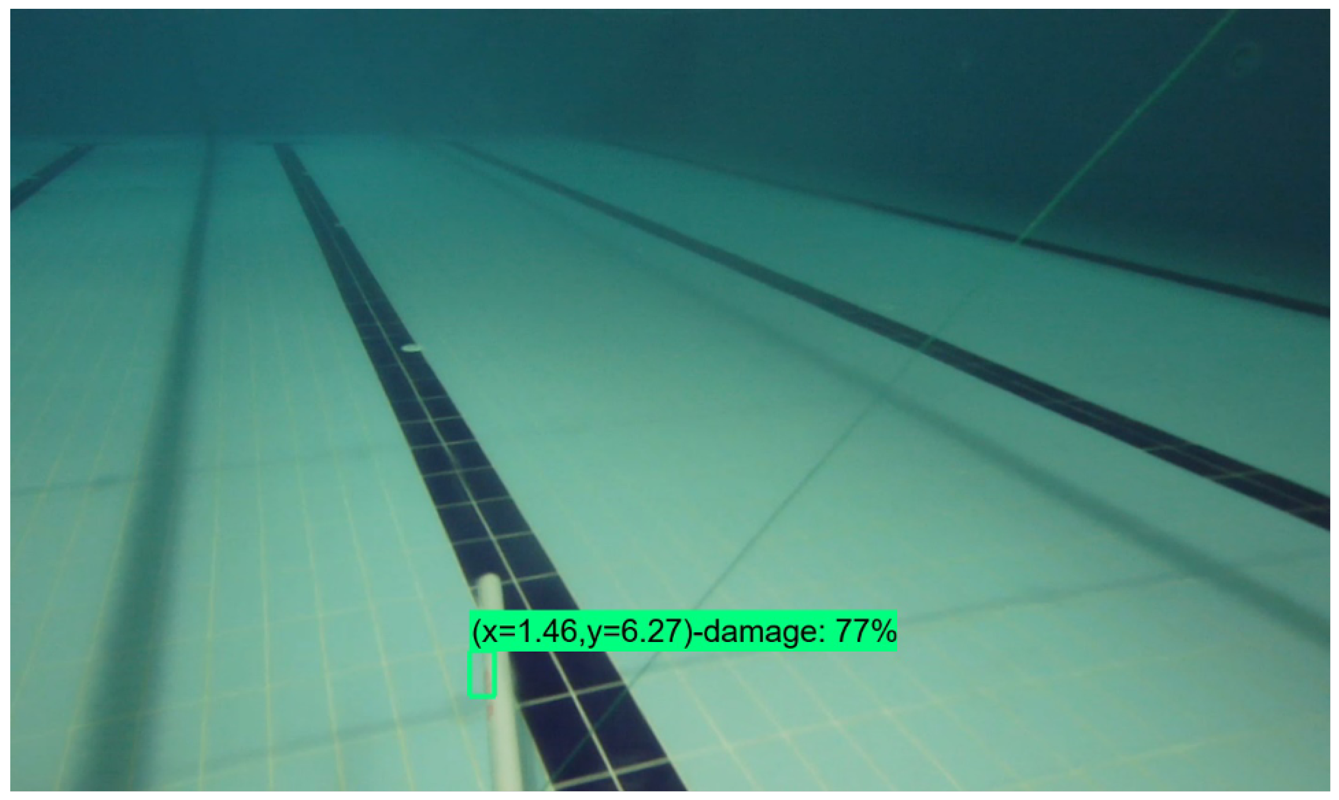
Figure 14.
Reference path (blue line) and followed path (red line)
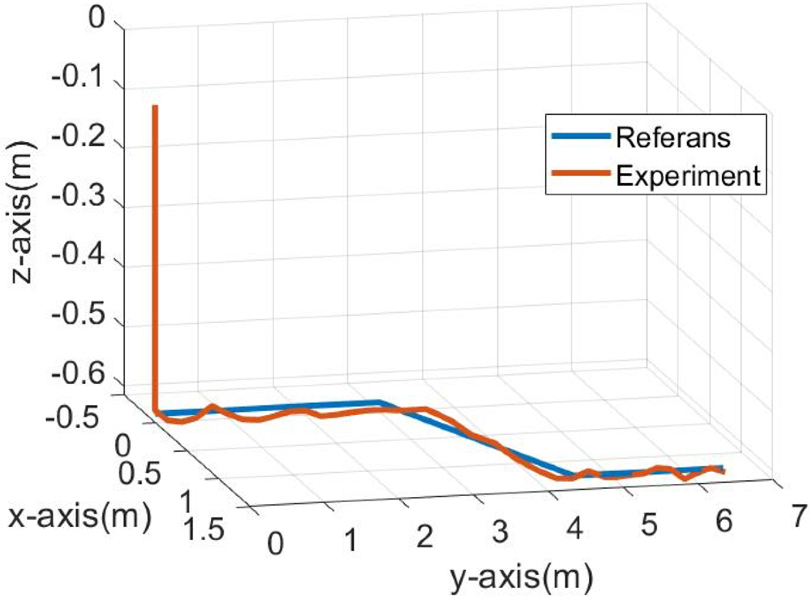

Table 1.
RMSE values between reference and tracked position value.
| Position | RMSE |
|---|---|
| x | 0.072 m |
| y | 0.037 m |
| z | 0.161 m |
| yaw | 1.9 deg |
Disclaimer/Publisher’s Note: The statements, opinions and data contained in all publications are solely those of the individual author(s) and contributor(s) and not of MDPI and/or the editor(s). MDPI and/or the editor(s) disclaim responsibility for any injury to people or property resulting from any ideas, methods, instructions or products referred to in the content. |
© 2024 by the authors. Licensee MDPI, Basel, Switzerland. This article is an open access article distributed under the terms and conditions of the Creative Commons Attribution (CC BY) license (http://creativecommons.org/licenses/by/4.0/).
Copyright: This open access article is published under a Creative Commons CC BY 4.0 license, which permit the free download, distribution, and reuse, provided that the author and preprint are cited in any reuse.


