Submitted:
19 August 2024
Posted:
19 August 2024
You are already at the latest version
Abstract
Euler's theorem about the relationship between the numbers of individual elements of planar graphs (vertices, edges, faces) is also satisfied when the graph has zero vertices. The problem of the existence or not of such graphs has so far been the subject of very few studies. Plus, research that didn't prove anything. The paper presents an interpretation of this kind of graphs as mathematical formations lying on piecewise smooth surfaces. The lines of intersection of two or more smooth surfaces (faces of a graph) form edges without a vertex of the graph. The elementary properties of such graphs are discussed, the method of counting non-isomorphic 0-vertex graphs and their importance in physics and chemistry are given.
Keywords:
chemical graph
; planar graph
; Euler's formula
; invariant states
MSC: 68R10 – 92E10
1. Introduction
1This work is dedicated to the memory of the tragically deceased Professor Ali Reza Ashrafi (1964 – 2023), an exceptional man and scientist.
A graph G is usually defined as a set of two sets, V and E [1,2]. The first, V = (v1, v2, …, vV) is called the vertex set of G; and E is a set of edges: E =(e1, e2,..,eE), where ek=(vi,vj), i.e. E is a subset of pairs of V elements. The sequence of vertices and adjacent edges is called a path. If in a given graph there are paths in which the first vertex is identical to the last one, then we say that the graph contains cycles (in particular, if there is only one vertex and one edge in the path, it will be a loop). Each cycle establishes two areas in the graph: inside the closed cycle and outside it. These areas are called the faces, F, of the graph. The number of faces of the graph, F =(f1, f2,…,fF) depends on the number of cycles, their mutual arrangement and on the Euler-Poincaré characteristic of the surface, χ(S), on which the graph is rearranged. At this point, I will add that in this work, the symbols V, E and F will be used to denote both sets defining the graph, as well as the number of elements in these sets.
The most common representation of graphs is their drawing on a two-dimensional surface with a specific topology, χ(S). If the drawing of G on a given surface can be made such that such a graph representation has no intersecting edges, then the graph is said to be flat on that surface. Euler's formula states [3] that if a finite, connected, planar graph is drawn in the plane without any edge intersections, then
v − e + f = 2. V+ F – E =χ(S)
In physics and chemistry, the most common surface on which to study the properties of graphs is the 2-D plane and the sphere isomorphic to it. The Euler–Poincaré coefficient χ(S) of these surfaces is 2. Therefore, the Euler equation for planar graphs is written in the form [3]:
V = E - F +2
In graph theory, formula (2) is most often used, e.g. to study the planarity of graphs with a large number of vertices or edges. It is not clear why so far no attention has been paid to the unclear situation of this equation for the case when V = 0, i.e. the problem of zero-vertex graphs. In graph theory, planar graphs with 0 vertices (as well as graphs with 0 edges), usually called null graphs or empty graphs [4], have an unclear definition. This is due to a lack of research on such graphs.
In particular, the number of such graphs remains inconclusive. It seems that this situation was caused by the tacit assumption of most researchers that graphs without vertices must also be without edges, i.e. that in fact there simply are no such graphs. The consequence of such an assumption is the statement that there is no problem, because there is no object that would cause this problem. In this work, we claim that the above statement is false, because graphs with 0 vertices exist and they are a natural complement to planar graphs in which V > 0. What's more, in such graphs we can see the existence of both graph-defining sets: V, E. What already absurd. A 0-vertex graph with a set of vertices V…? So that it does not look like delusions, I will add that the graphs mentioned above play a role in explaining phenomena in some areas of physics and chemistry [6].
2. Theory
Before we move on to the search for planar 0-vertex graphs on 2-D piecewise smooth surfaces, let's articulate what we are looking for. The answer results from equation (2), we are looking for graphs in which the number of edges, E, is 2 less than the number of faces F:
E = F - 2
For the sake of clarity, let me remind you that a face of graph is a smooth fragment of a 2-D surface, and an edge is a line separating the graph faces. If such a 2-D geometric object with properties (3) is immersed in a space with dimensions n = 3, 4, ... etc., then it will be natural to conclude that they arise as a result of various topological operations performed on natural two-dimensional surfaces in the considered spaces. Natural two-dimensional surfaces are all planes spanning individual pairs of coordinate axes: [z= v= …=0, (x= s, y= t); 0 ≤ s, t <∞], …. . Figure 1a and b show these planes in spaces with n=3 and n=4.
All natural planes of a given space meet at one point called the invariant point (in geometry, it is the origin of the coordinate system). In this and subsequent drawings, this point is marked with an asterisk. Some of these planes are cut along straight lines. The set of all natural planes of n-dimensional space (it has n*(n-1)/2 elements) creates an n-1 dimensional geometric object. Some of the elements of the set will create a smooth 2-D surface in pieces. Each smooth piece of this surface is adjacent to only two others (because the created surface is 2-dimensional!). In 3-D space, all 3 normal planes create a 2-D surface that is piecewise smooth. In 4-D space, only 4 out of 6 possible ones create such a surface (because there are so many possible planes spanning 4 pairs of axes, so that each plane is adjacent to two others). In general, in n-D space, only n planes create a piecewise 2-D structure. Transformations such as translations, rotations, and other topological operations performed on smooth 2-D pieces of surfaces constructed in this way transform them into geometric objects isomorphic with the initial ones. Therefore, the parameter χ(S) of the objects created in this way will be equal to 2. Let the surfaces created as a result of these transformations describe the functions: F1(x,y), F2(x,z), F3(x,v), ...,F4(y, z), F5(y,v), …. In a 3-dimensional space, these functions can be transformed into three intersecting pairs of functions of two variables: f1(x,y), f2(x,y), f3(x,y). Figure 2a shows these features.
The figure shows that a piecewise smooth 2-D object consists of three planes (generally these will be 2-D surfaces) intersecting along 3 lines. The planes are the faces, the intersection lines are the edge(s) of the graph thus created. This would suggest that this graph has 3 faces and 3 edges and no vertices. According to Eq. 3 such a graph structure would lead to the conclusion that this object cannot be planar. This conclusion, however, is incorrect because it resulted from the analysis of the properties of planar graphs on smooth surfaces. On the latter, only two faces can always be adjacent to each other, so individual edges in such a situation separate only 2 faces. Figure 2a shows that, in a 2-D piecewise structure, also three faces can be adjacent to each other at the same time. Therefore, it should be assumed that all three lines separating three faces constitute one edge, i.e. they constitute a 0-vertex graph. The projection of this graph onto the plane is shown in Figure 2b. We will call such a projection a 0-vertex graph map, or a graph-map.
In this way, we come to the conclusion that in 3-D space, on surfaces that are partially smooth, one edge consists of the intersection lines of adjacent faces. So if three faces are adjacent to each other at the same time, then the edge will have a bifurcation at the invariant point. The last sentences can be recapitulated by the statement: "Zero-vertex graphs exist on 2-D piecewise surfaces. In a 3-dimensional space, such a graph is formed by three intersecting planes, i.e. faces of the graph. The only edge of this graph is formed by the intersection lines of the faces. Therefore, this edge exhibits a bifurcation at the invariant point”. Let us now move on to the form of edges in 0-vertex graphs in a space of larger dimensions. Since these edges create lines of intersection between adjacent faces, it is expected that there are 3 types of edges:
-edges consisting of only one intersection line starting from the invariant point (see Figure 3a);
-edges composed of two intersection lines passing through the invariant point (see Figure 3b);
-edges with bifurcation at the invariant point composed of 3 intersection lines (see Figure 3c).
Let us emphasize here that bifurcation edges appear not only when three faces are adjacent to each other at the same time. Such edges are a consequence of more subtle relationships between the faces of the graph. What are these relationships? We will find the answer by considering example pairs of faces:
-the faces described by the equations {F1(x,y), F2(z,v)} do not intersect, the only common point of these faces is the invariant point. So such a pair of faces cannot participate in the formation of a 2-D piecewise smooth structure.
-the faces described by the equations {F3(x,y), F4(y,z)} intersect along the line z =ϕ(x). Such a pair of faces can participate in the creation of 2-D piecewise smooth structure, and the length of the intersection line of the faces is measured by the value of the "z" component of this line: z =ϕ(x).
-the faces described by the equations {F5(x,y), F6(y,v)} intersect along the line v =ϕ(x). Such a pair of faces can participate in the creation of 2-D piecewise smooth structure, and the length of the intersection line of the faces is measured by the value of the "v" component of this line: v =ϕ(x).
Therefore, the edges of graphs on smooth surfaces will be created from one type of intersection line. These will be edges of the following types: "z", "v", "w", ..., etc. In the "pictorial" representation of such graphs, individual edges can be represented by drawing them with different lines. Now we can formulate the answer to the question what relations between the faces are responsible for the formation of edges with bifurcation. Well, "if the lengths of the three intersection lines of the faces are determined by the component relative to the same axis, then these lines form an edge with a bifurcation. In 3-D space, this situation occurs when all three faces are adjacent. However, when the dimension of the space is > 3, the only condition for the existence of an edge with a bifurcation is that three intersection lines of the faces belong to one category.
Let's return to the main topic, which is the representation of flat 0-vertex graphs in spaces with dimensions: n = 4, 5, 6 and more dimensions. Graphs in such spaces will have n -2 edges made of 1, 2, or 3 of all n intersection lines. So the number of these objects, ηo, will be equal to the number of ways to divide n faces by n-2 edges. Figure 4a shows that for the case n = 4 there will be ηo = 3 different face divisions. This means that there are three non-isomorphic 0-vertex graphs in 4-D space (Figure 4b shows graph maps of such graphs).
The problem of counting 0-vertex graphs with n faces practically comes down to counting different graph-maps of such objects. This is not a difficult matter, but it is burdensome due to the lack of vertices in these objects. Therefore, before we move on to this problem, let us consider whether the objects considered here are indeed graphs according to the classical definition: "graph = a set of two sets".
After all, if there are no vertices in such graphs, they have neither a set of vertices nor a set of pairs of vertices, i.e. edges! This is indeed the case, but these structures have intersecting faces. Let us consider the situation presented in Figure 2a. In order not to complicate things unnecessarily, we will only consider one: f1(x,y), f2(x,y), out of three possible pairs of intersecting planes. Let the values of the functions defining the faces be marked as follows:
z1= f1(x,y), z2= f2(x,y)
Let the points lying on the first and second plane be marked: ϑ1, ϑ2. The line of intersection of both faces runs from the invariant point, with coordinates marked s*, to ∞. The position of the points lying infinitely close to the line on both faces is defined by the equations:
The lower limit of the s parameter results from the fact that in Figure 2a the functions defining the faces are monotonically decreasing functions. The choice of monotonically increasing functions would not bring any significant changes for the case in question. Let us consider the set of points ϑ1, ϑ2 lying on both sides of the intersection of the planes. In fact, this infinitely large set can be denoted, and called the set of vertices:
V =( ϑ1(s), ϑ2 (s); -∞ < s ≤ s*)
If a pair of vertices lying on both sides of the intersection line are combined into a pair marked e12:
then an infinite set of such pairs creates a set of edges, E, connecting both faces:
e12 (s) =( ( ϑ1(s), ϑ2 (s)); -∞ < s ≤ s*)
E=( e12(s); -∞ < s ≤ s* )
In this way, every 0-vertex graph is transformed into a set of two infinitely large uncountable sets: points lying on the edge of both intersecting planes, i.e. vertices, V, and pairs of these points, E, i.e. edges: G = (V, E). That is, 0-vertex graphs can in fact be treated as a set of two infinite sets: vertices and edges. And this is the classic definition of a graph. This way of looking at the objects considered here tells us that they are, in fact, graphs.
Figure 5 shows all graph-maps for the number of edges E = 1, 2, 3. From the second column of Figure 5 we can see that for E = 1 there is only one 0-vertex graph; for E = 2 there are already 3; and for E = 3 there are 5 of them. As I noted earlier, the problem of counting, i.e. finding the number of different, i.e. non-isomorphic graphs with a given number of edges, comes down to finding the number of different ways of arranging E edges around the invariant point, each of these ways should divide area on E + 2 faces. This seems to be a tedious matter because the objects we are examining do not have vertices. Therefore, in the works [6,7] it was proposed to replace these graphs representing them with "normal" graphs having, like any "racial graph", vertices, edges and faces. If the considered 0-vertex graphs are marked with the letter G, and the corresponding normal graphs are marked with G*, then the correspondence G* ↔ G will be obtained by replacing the sets:
V* ↔ E = F-2
E* ↔ F
Well, you might say, where is the appropriateness for F*? Well, we get the number of faces in a normal graph by inserting V* and E* into Euler's equation (1). It is easy to see that in such graphs F* = 4, regardless of how many faces and edges there are in the 0-vertex graph!
The third column in Figure 5 shows all normal graphs corresponding to 0-vertex graphs with the number of edges E < 4. When searching for all non-isomorphic normal graphs, remember that they always have four faces and the number of vertices in them is the same as the number of edges, in the corresponding 0-vertex graphs. The valence of each vertex is even, which is a consequence of the fact that each edge of a 0-vertex graph is created by the intersection of an even number of faces. The work [6] shows all normal graphs for E < 9. The work of finding normal graphs is facilitated by the obvious recursion that allows determining the form of an n + 1 vertex graph by appropriately inserting a new vertex at individual edges of the n-vertex graph.
Table 1 gives the number of all normal graphs, ηo, for E < 9. The table indicates that the values of ηo(E) constitute an increasing numerical sequence. An elementary analysis [8,9] of the sequence shows that for even values of E = 2k, k = 0, 1, 2…, the value of ηo differs by k(k + 3) / 2 from the corresponding value for both neighboring systems when E is odd (i.e., E =2k - 1 and E = 2k + 1):
ηo(2k) - ηo(2k-1) = ηo(2k+1) - ηo(2k) = k(k+3)/2, where k = 1, 2, 3, 4
This correspondence, along with the boundary value ηo(E = 1) = 1, gives the following number of non-isomorphic normal graphs:
ηo(E=2k) = 3+2*(k -1)(k +1)+k*(k -1)(2k -1)/6, where k =0, 1, 2, 3,…
ηo(E=2k+1) = ηo(E =2k)+k*(k +3)/2,
From equations (13), (14) it follows that the number of non-isomorphic normal graphs, and therefore the number of 0-vertex graphs corresponding to them, increases approximately as (E)3. This is not a very fast growth compared to the growth of other types of planar graphs. However, in the author's opinion, counting the graphs considered here is an extremely tedious and burdensome work, and without the help of normal graphs it would be practically impossible for E > 5.
3. Summary
The existence of flat 0-vertex graphs on smooth 2-D surfaces has been questioned. The work shows that taking into account 2-D piecewise smooth surfaces leads to the conclusion:
- such graphs exist and are formed by smooth surfaces intersecting at one point, i.e. faces of such graphs;
- intersection lines of faces form the edges of 0-vertex graphs;
- in this way, all edges in such graphs pass through the invariant point;
- there are only 3 types of edges in planar 0-vertex graphs, among these types the singularity is an edge with a bifurcation at the invariant point;
- the number o(E = n-2) of 0-vertex graphs depends on the dimension of the space, n, in which there is a 2-D piecewise smooth surface;
- a formula was found to count the number of graphs considered here (see Eqs. 13, 14);
- it was noticed that there is a clear correspondence (see Eqs. 10, 11) between 0-vertex graphs and "normal" graphs with vertices - in which the number of faces is always constant and equal to 4.
Okay, you could say, but what does this have to do with chemistry or physics? Well, about a hundred years ago, a certain connection between planar graphs and thermodynamic equilibrium was noticed [10], which, as we know, is determined by the f values of parameters, called degrees of freedom. During these hundred years, this connection has been analyzed by various research groups [5,11,12,13,14,15,16,17,18]. The summary of this analysis is the statement that the thermodynamic equilibrium is represented by a f -vertex planar graph. Let's omit the equilibrium in which f > 0, because the case of graphs with the number of vertices greater than zero is clear, let's stop at the equilibria in which f = 0. In thermodynamics, such an equilibrium state is called invariant. If it exists, and no one can have any doubts about it, then in the light of what has been written above, it should be represented by a flat 0-vertex graph. And the latter were not noticed in graph theory until recently. Indeed, their existence was denied! The work presented here shows that the existence of such graphs cannot be denied, if we assume that such graphs lead their "mathematical existence" not only on smooth flat surfaces, but also on surfaces with smooth pieces. In the earlier work [6] the relation of such graphs to thermodynamic equilibrium in complex physicochemical systems with an arbitrary number of components, C, was described in more detail. The aforementioned work shows, for example, that 0-vertex graphs allow us to determine which invariant equilibrium states are thermodynamically allowed and which are forbidden; what is the composition of the individual phases in these states; and what is the number of different types of invariant states in systems containing C components. In the opinion of the author, this is enough to appreciate the role of 0-vertex graphs and topologies in understanding chemical thermodynamics.
References
- R. Diestel, Graph Theory, Springer-Verlag New York 1997, 2000.
- N. Trinajstic, Chemical Graph Theory, CRC Press, Boca Raton, 1992.
- L. Euler, "Elementa doctrinae solidorum" (1758). Euler Archive - All Works. 230. https://scholarlycommons.pacific.edu/euler-works/230.
- F. Harary, R.C. Read, Is the null-graph a pointless concept? Graphs and Combinatorics in Lect. Notes Math. 406 (1974) 37-44. [CrossRef]
- J. Turulski, Dimension of the Gibbs function topological manifold, J. Math. Chem. 53 (2015) 495-513. [CrossRef]
- J. Turulski, Number of Classes of Invariant Equilibrium States in Complex Thermodynamic Systems, Amer. J. Chem. Phys. 8(1) (2019) 17-25. [CrossRef]
- J. Turulski, On Selected Properties of the Gibbs Function Topological Manifold, Iranian J. Math. Chem. 13 (3) (2022) 253 – 280. [CrossRef]
- N.J.A. Sloane N.J.A., S. Plouffe, The Encyclopedia of Integer Sequences, Academic Press, NY, 1995.
- J.H. Conway, R.K. Guy, The Book of Numbers, Springer Verlag, NY, 1998.
- Rudel, The phase rule and the boundary law of Euler, Z. Electrochem. 35 (1929) 54-57.
- M.A. Klochko, Analogy between phase rule and the Euler theorem for polyhedrons, Izvest. Sektora Fiz-Khim. Analiza, Inst. Obshch.Neorg.Khim.Akad.Nauk SSSR 19 (1949) 82-88.
- D.R. Rouvray, Uses of graph theory, Chem. Br. 10 (1974) 11-15.
- T.P. Radhakrishnan, Euler's formula and phase rule, J.Math.Chem. 5 (1990) 381-387. [CrossRef]
- L. Pogliani, Phase diagrams and physiochemical graphs MATCH Commun. Math. Comput. Chem. 49 (2003) 141-152.
- A.I. Seifer, V.S. Stein, Topology composition-property of diagram phase, Zh. Neorg. Khim. 6 (1961) 2711-2723.
- J. Mindel, Gibbs' phase rule and Euler's formula, J.Chem. Edu. 39 (1962) 512-514. [CrossRef]
- F.A. Weinhold, Theoretical Chemistry, Advances and Perspectives, vol. 3, (Eds.: H.Eyring, D. Henderson), Academic Press, NY, 1978, p. 15-54.
- J. Turulski, J. Niedzielski, Use of graph theory in thermodynamics of phase equilibria, J. Chem.Inf. Comput. Sci. 42 (2002) 534-539. [CrossRef]
Figure 1.
Natural two-dimensional surfaces are 2-D planes stretched on individual axes of the coordinate system. There are n*(n-1) such surfaces in n-dimensional space. Figure 1a shows these objects in 3-D space; Figure 1b – in four-dimensional space. In n-D space, only n of these surfaces create a two-dimensional piecewise smooth surface.
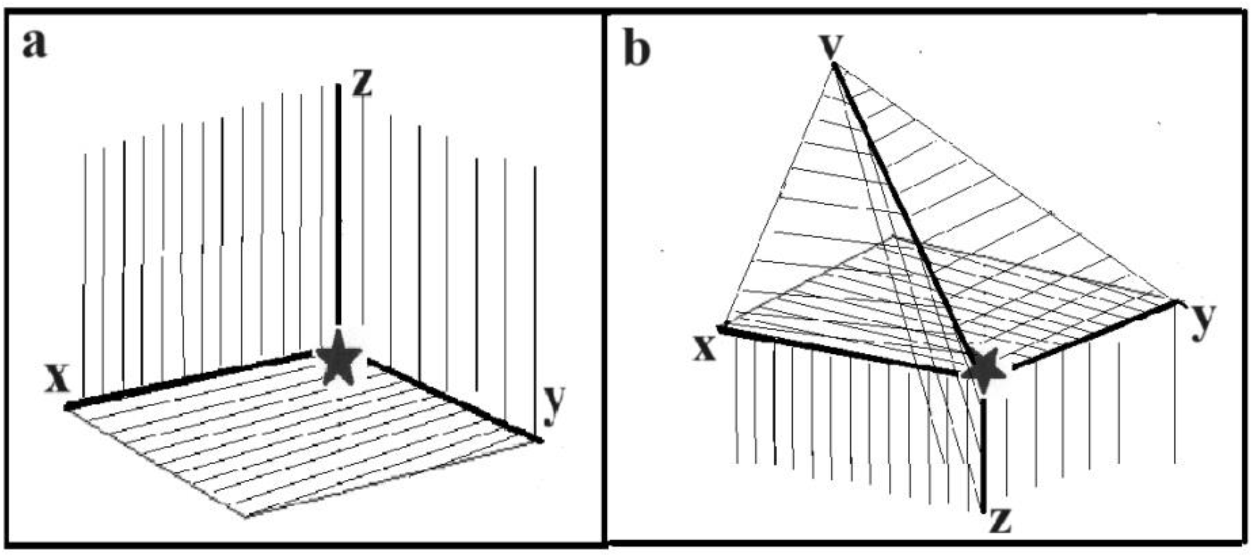
Figure 2.
Figure 2a: An example of a 2-D piecewise smooth surface in three-dimensional space created by topological transformation of natural surfaces in this space. The smooth pieces of this structure are faces, while the intersection lines of the faces constitute the edge of the graph without vertices. Therefore, such a geometric formation is a 0-vertex graph. The edge in this graph exhibits a bifurcation at the intersection of all faces. Figure 2b: graph map resulting from the projection of a 0-vertex graph onto a plane.
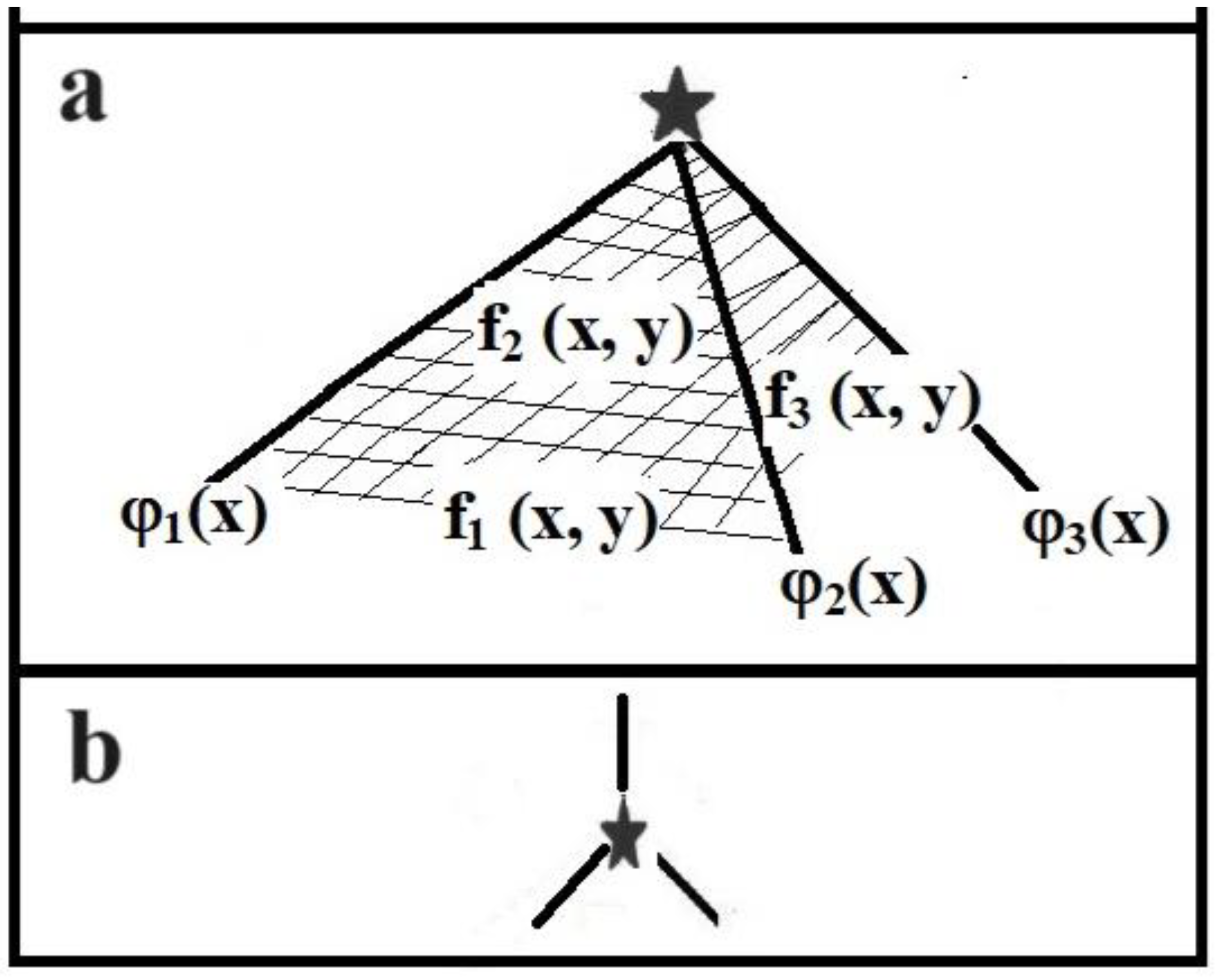
Figure 3.
All possible types of edges in 0-vertex graphs. Figure 3a: the edge leaving the invariant point is formed by one line of intersection of two faces of the graph; Figure 3b: a family of edges passing through the invariant point composed of two intersection lines of four faces; Figure 3c: the edge showing bifurcation at the invariant point is formed from three intersection lines of 3 (in 3-D space) or 4 faces.
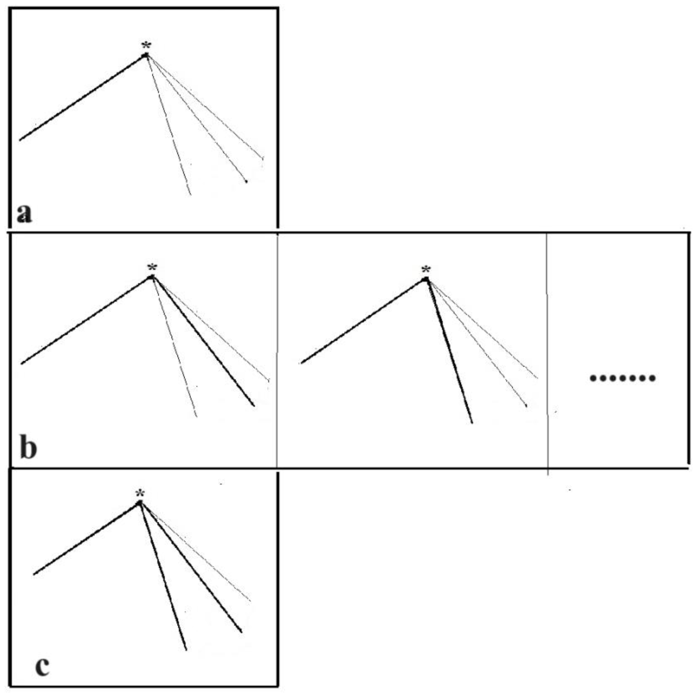
Figure 4.
Figure 4a: Example 2-D piecewise smooth surfaces in four-dimensional space created by topological transformation of natural surfaces in this space. The smooth pieces of this structure are the faces, and the intersection lines of the faces are the two edges of the 0-vertex graph. The first edge of the graph is marked with a solid line, the second - with a dashed line. So there are three non-isomorphic 0-vertex graphs in 4-D space. Figure 4b: graph maps resulting from the projection of 0-vertex graphs onto a plane.
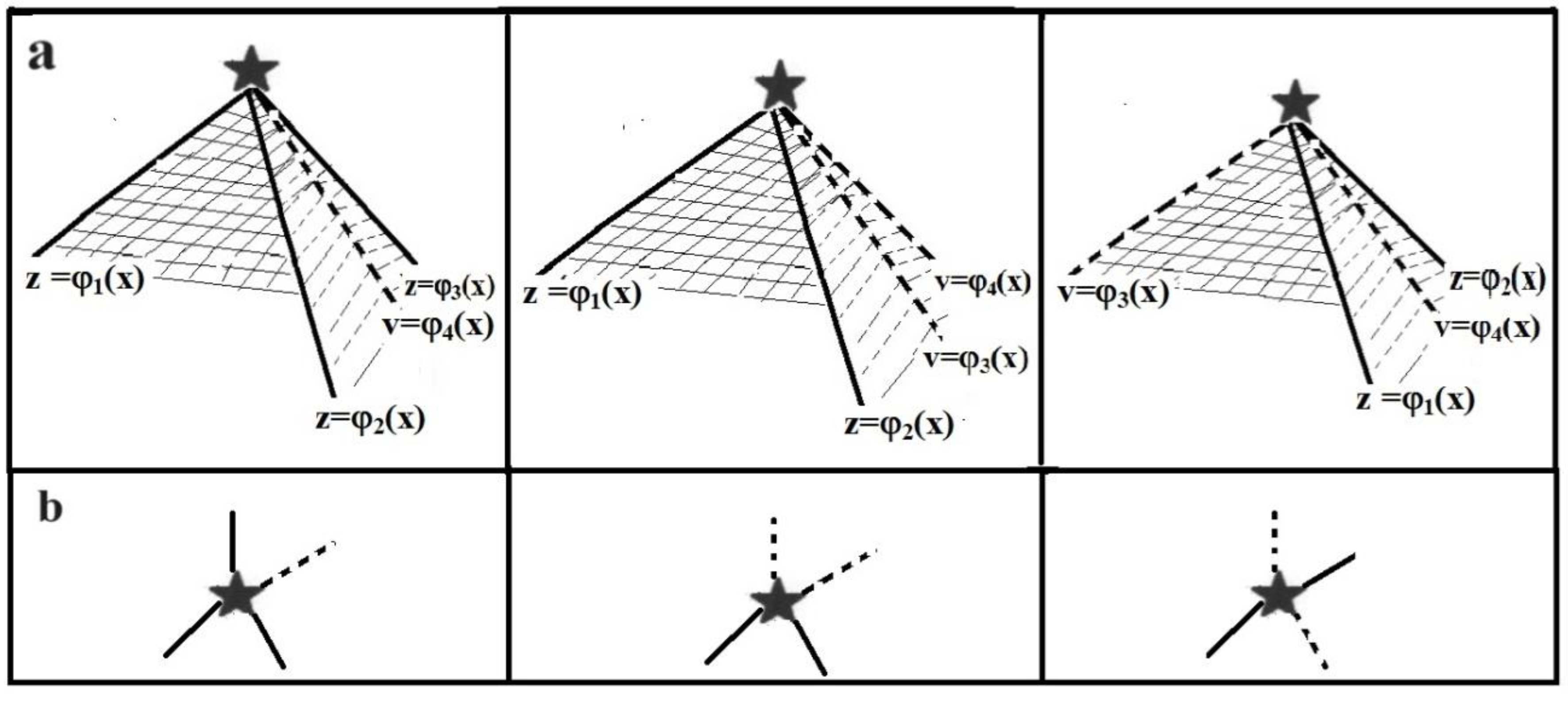
Figure 5.
All possible graph-maps, G, of 0-vertex graphs and the corresponding normal graphs, G*, allowed in 3-, 4- and 5-dimensional spaces. Each edge in G is marked with different lines. The last column of the table gives the value of ηo, i.e. the number of non-isomorphic graphs in a given space.
Figure 5.
All possible graph-maps, G, of 0-vertex graphs and the corresponding normal graphs, G*, allowed in 3-, 4- and 5-dimensional spaces. Each edge in G is marked with different lines. The last column of the table gives the value of ηo, i.e. the number of non-isomorphic graphs in a given space.
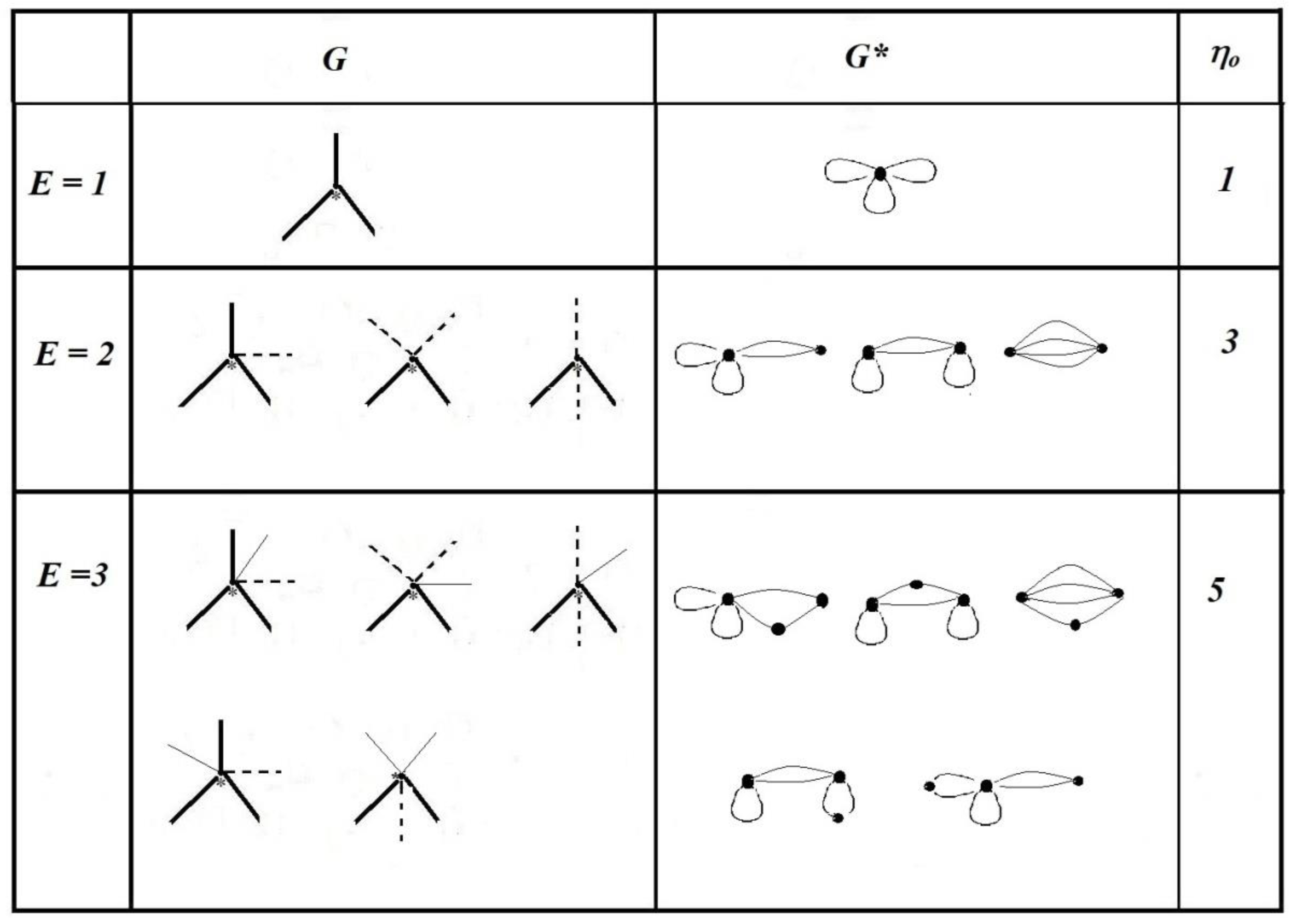

Table 1.
Number of 0-vertex graphs, ηo, for systems with no more than 8 edges (E ≤ 8). The parameter Δ=|ηo(2k) - ηo( 2k± 1)| indicates that the ηo for E with an even number o differs by the same amount from both of its neighbors with an odd number E.
Table 1.
Number of 0-vertex graphs, ηo, for systems with no more than 8 edges (E ≤ 8). The parameter Δ=|ηo(2k) - ηo( 2k± 1)| indicates that the ηo for E with an even number o differs by the same amount from both of its neighbors with an odd number E.
|
k |
0 |
1 |
2 |
2 |
3 |
3 |
4 |
4 |
… |
k |
|
|
E =2k+1 E =2k |
1 |
2 |
3 |
4 |
5 |
6 |
7 |
8 |
… |
2k |
2k+1 |
| ηo | 1 | 3 | 5 | 10 | 15 | 24 | 33 | 47 | … | Eq. (12) | Eq. (13) |
| Δ | 2 | 5 | 9 | 14 | k(k+3)/2 |
Disclaimer/Publisher’s Note: The statements, opinions and data contained in all publications are solely those of the individual author(s) and contributor(s) and not of MDPI and/or the editor(s). MDPI and/or the editor(s) disclaim responsibility for any injury to people or property resulting from any ideas, methods, instructions or products referred to in the content. |
© 2024 by the authors. Licensee MDPI, Basel, Switzerland. This article is an open access article distributed under the terms and conditions of the Creative Commons Attribution (CC BY) license (http://creativecommons.org/licenses/by/4.0/).
Copyright: This open access article is published under a Creative Commons CC BY 4.0 license, which permit the free download, distribution, and reuse, provided that the author and preprint are cited in any reuse.


