
Submitted:
19 August 2024
Posted:
19 August 2024
You are already at the latest version
Abstract
In some clinical applications pulsating currents are delivered into a body region for therapeutic purposes.
In this paper we analyze the generated thermal field with the aim of determining the amplitude, period and duration of those stimuli, guaranteeing that the temperature of the interested tissue stays below the necrosis threshold.
Keywords:
electric pulses
; blood perfusion
; safe operational ranges
1. Introduction
In some clinical procedures electric pulses of moderate intensity (up to V) are applied to biological tissues. Consequently, temperature may raise locally by some degrees. This phenomenon is generally negligible, but it should be kept under control, particularly for long lasting procedures, since it is known that cells exposed for long time to temperatures exceeding may die, thus inducing necrosis. This is not a strict rule in the sense that different tissues have different sensitivity to heat and, for the same tissue, the reaction may vary from patient to patient. For a general review on this extensively studied subject see, e. g., [1], Chapt. 6. Here we want to formulate a simple mathematical model to predict the steady state temperature attained in a tissue in which electric power is delivered in the form of pulsating voltage by means of a bipolar device, so that current is mainly concentrated in the region between the active electrodes, which are a few millimeters apart. We will point out that a critical quantity in determining the maximal temperature is the local acidity level, since it strongly influences electric conductivity. While in normal conditions heating will be proved to remain generally confined within safe limits, when the environmental pH is low, the selection of the stimulating parameters requires particular attention. We will derive the approximate range in which the pulse amplitude, period, and duration can be chosen, indicating which values may turn out to be dangerous, depending on the local pH level. We will perform a two-step approach: first neglecting and then including the stabilizing effect of blood perfusion.
2. The Physical Setting and a First Approach
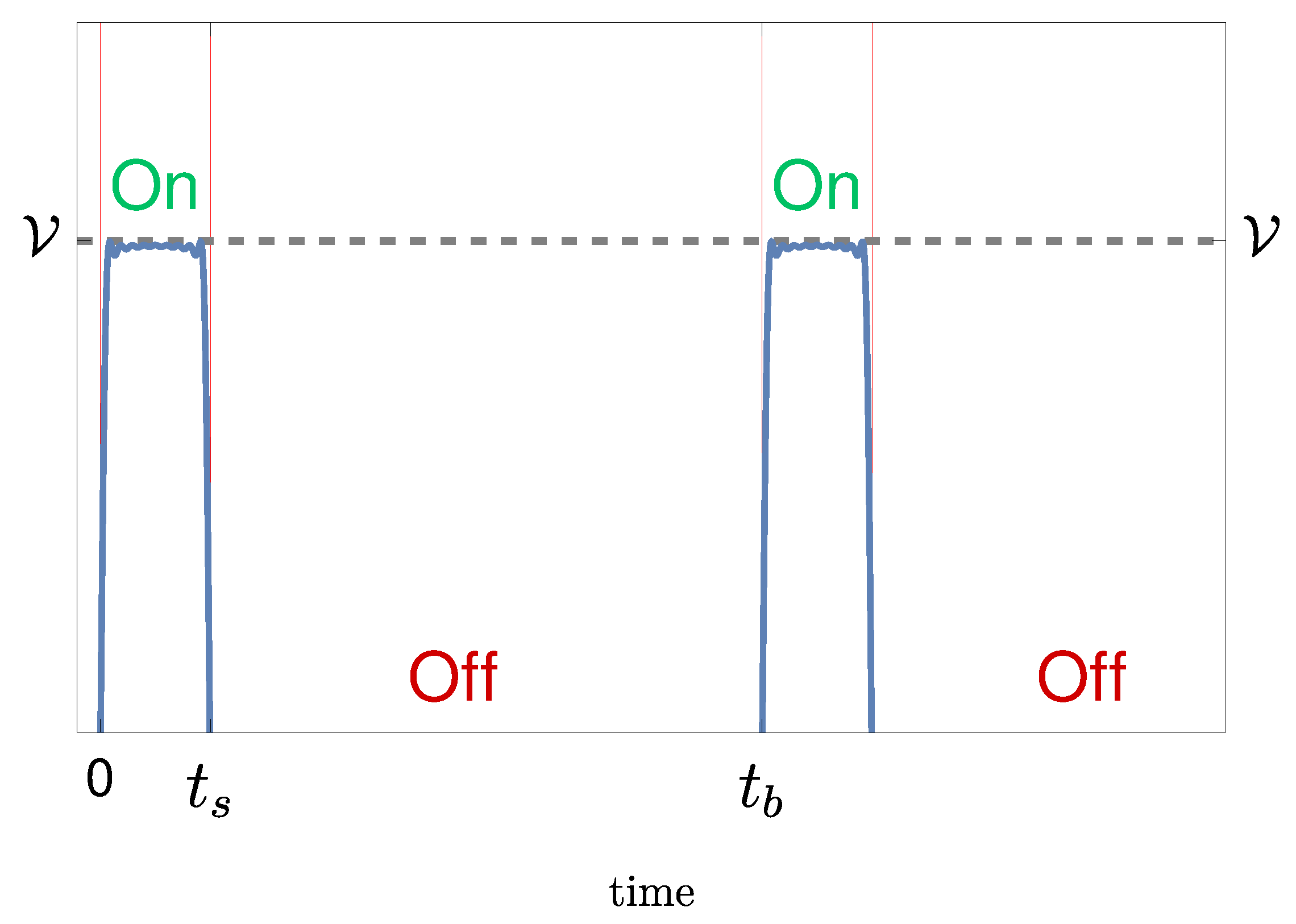
We consider the case in which the electrodes are introduced in a body cavity, generating a pulsating electric field for therapeutic purposes. Of course the electric field extends over the whole body, but it fades away rapidly far from the source. A first simplifying assumption we make is to suppose that heat is generated by a uniform pulsating current confined in a spherical region of radius R around the electrodes. The current has a duration and a period . In our approach the power delivered is considered constant, i.e. averaged over a period, considering that (<2 s) is much shorter than the application time (hours).
Figure 1.
Delivered voltage versus time for a given voltage and a given duty cycle (ratio of the pulse duration over the time it takes the signal to complete an on-off cycle).
Figure 1.
Delivered voltage versus time for a given voltage and a given duty cycle (ratio of the pulse duration over the time it takes the signal to complete an on-off cycle).
Next, we add the assumption that heat diffuses out of such a sphere through a larger sphere of radius (for instance ; typically mm, cm, see Figure 2), whose boundary has a constant temperature , representing the patient’s basal temperature. Doing so we neglect the possible tissue thermal inhomogeneity, a fact of not great importance in the framework of the approximation we are aiming at. If is the radial coordinate and is time, the temperature obeys the equation
where denotes the power rate per unit volume, namely
The symbol Q denotes the average power delivered into the sphere because of Joule effect. We recall that is density (kgm), c is specific heat (Jkg−1), k is thermal conductivity Wm(). The equation is supplemented by the boundary conditions for and for (i.e. no heat flux through the center, by symmetry). Temperature and heat flux are continuous across the interface .
We select
as a characteristic length (in SI units) for the present problem. Then, we rescale and as follows
where has to be conveniently chosen. Finally we summarize the dimensional typical values of the physical quantities involved in the case of human tissues:
Let us rewrite equation (1) in the following form, where we have set :
where denotes the Heaviside function. Note that we have extended the outer domain to infinity, neglecting the influence of the boundary , just making use of the fact that . The solutions that will be presented are meant to be the leading order approximations when terms of the order of are neglected. We identify as the procedure duration, hence
Thus, (3) entails (stationary state)
We define
measured in Kelvin degrees. During stimulation, the power supplied is , where is the stimulation amplitude and is the impedance. Thus, keeping into account that the voltage is applied only during the time during each period, we have
We may write , where is the medium electrical conductivity (measured in S, S=Siemens) and L can be taken as the side of a cubic box whose volume is equal to that of the sphere of radius R, i. e. . Consequently, we can rewrite (6) as
where
The expression (7) of the source term emphasizes the role of the three parameters settable by the operator and of the physical properties of the medium entering as the ratio , thus indicating that the two conductivities act in opposite ways.
Though the radius R has eventually disappeared from our main estimates, it is interesting to check that our guess ( mm) was sensible. People working in the area of electrostimulation (see, e.g. [2]) normally take the empirical assumption that the resistive load offered to the generator is . So far we did not make any use of this information because it is too generic, but it can give a reasonable idea of the size of R, using . Setting now (as we shall see for the normal environment), and , we get mm, which is of the same order of magnitude of our guess.
Taking into account the boundary and interface conditions for , the differential system to be solved for is
It can be easily checked that the solution writes
Notice that function is always and takes its maximum for . Using , we can rewrite (10) as
Figure 3 and Figure 4 show how changes by changing the operational parameters, considering a reasonable range for (generally 0.4 but exceptionally up to 2 or more), , and the instrument operational intervals ( V, ms, and ms).
Working with the temperature at the center may however be too heavy a condition, since the sphere of (dimensionless) radius is more likely occupied by a liquid medium, the cellular tissue being more or less at the boundary of the ideal sphere in which we have confined the current. Therefore, a more interesting temperature seems to be the one calculated at (see Figure 3 and Figure 4), namely, from (10),
It is reasonable to suppose that (12) provides the maximal temperature difference to which the tissue is exposed. Our goal now is to investigate the safety condition , where a conservative value for could be .
3. Safety Stimulating Conditions
Let us define
so that the safety condition becomes
While the thermal conductivity k for biological tissues is more or less constant with typical value (with the exception of fat, see, e. g., [3]), the electrical conductivity is strongly affected by the pH of the ambient. We may first assume that the conductive medium filling the sphere of radius R is aqueous (e.g. saliva, as it happens in the esophagus). In that case, the paper [4] provides for values between and . Passing to SI units (=), we take a typical value . Thus, for , the safety condition (14) is to be read
This result has to be examined in view of the range of the parameters practically available on the devices employed.
If we set , then condition (15) entails, approximately,
where .
The interval of positiveness of the function identifies the safety ratio for any given , or, vice versa, the safe voltage for any given ratio . Figure 5 and Figure 6 show, respectively, the cases V and .
This result indicates that the procedure is feasible even with the largest stimulation amplitude (), but with a suitable control of the ratio (for instance, if s then ms would be fine). According to (12), the adoption of the extreme values settable on the generator (V and ) gives a maximal temperature increase of about , which is far beyond criticality. Therefore it is not suggestible to set the generator parameters at their extreme values, though it would be sufficient, e. g., to keep the pulse duration sufficiently low.
A much worse scenario is offered when current flows in an acidic medium, like gastric juice. In the paper [4] the value of the gastric juice electrical conductivity was measured vs. pH and a typical value was found to be , i.e. 5 times larger than the one of saliva. Clearly, the safety condition is now more severe, namely , thus (16) modifies (still approximately) to
Figure 7 and Figure 8 refer to this case, showing that the range of admissible selectable parameters is severely reduced.
For instance the lower limit for x corresponding to raises to 68.5, which almost nullifies the therapeutic effect on the patient. In correspondence to the constraint on is , which is, in most cases, ineffective, making the procedure practically impossible. To have an idea on how to proceed in this case let us revert to the expression (12) of the critical temperature with , namely
With an effective value and requiring a maximum value for of, say, , the choice for the ratio must be such that , which is reasonable. Thus, still in this unfavorable situation there is a way to safely perform the procedure, but selecting the voltage and the time parameters with care. Taking the extreme values and would produce, in this case, a temperature increase greater than , which is unbearable. The conclusion is that pulsed current stimulation of biological tissues is normally safe, but it may become critical in the presence of highly conductive (i.e. acidic) media. Stimulating at high voltage and with pulse duration close to the stimulation period requires that local pH value be previously checked and the ratio x suitably selected.
4. Introducing the effect of blood perfusion
Blood circulation has a stabilizing effect on temperature. In the specific case, it helps removing heat from the interested region. This feature can be introduced in the model by modifying the source term in equation (1) as follows: if (unchanged) and (b=blood), for , representing the heat removing rate. Clearly, has dimension and so has dimension . Indeed is the volume of blood crossing the unit volume of tissue in one second. For soft tissues we can take or less (see [5,6,7]). Thus, the differential equation governing the temperature evolution is obviously the same, namely (1), but now (2) is replaced by
Proceeding as in the Sect. Section 2, we first rescale with R and with (see (4)), so to formulate again the problem in the steady state and in an unbounded domain. Finally, we introduce so that the new system of differential equations to integrate is the following
Here (dimensionless). Recalling the estimate , , and that
we obtain , i. e. . The solution of system (19) in terms of writes as follows
Figure 11 shows that blood perfusion entails a significant reduction of the thermal fields given by (10). It is worth noting that if tends to zero the no-perfusion solution is retrieved.
Let us analyze the influence of perfusion on the safety conditions. From (20) we get
which clearly emphasizes the influence of perfusion: the corresponding relative change as a function or r is
hence (see Figure 12).
Accordingly, the safety condition (15) changes as follows
which, for , , , and entails
showing some improvement with respect to the no-perfusion case. For instance, for this implies , allowing e.g. to increase to when . Similarly, for we require
with a certain improvement with respect to the corresponding condition (16).
In addition to safety conditions it is reasonable to add some efficacy condition, because if is too small or x is too large the treatment may not be effective. Thus, we impose the constraints and (for instance , ) and possibly also the lower limit . In view of these requirements, the suggestible parameters range are further reduced. Figure 13 shows the no-efficacy region when the above conditions are imposed for the respective cases , .
5. Conclusions
We have formulated a mathematical model to predict the temperature increase caused by the application of a pulsating current in a body compartment, supplied in situ by a bipolar device. This issue is important in view of the fact that cells can die when exposed to temperatures of C for long time. The main finding is that local acidity is a crucial quantity. Lowering pH (e.g. for a gastric reflux) may raise electrical conductivity to such a point to make the treatment dangerous if the stimulating parameters are not selected with care. We computed the safety ranges for amplitude, duration, period of the voltage pulses in correspondence to normal pH and to low pH, based on the data provided by the literature.
Author Contributions
Angiolo Farina, Antonio Fasano and Fabio Rosso performed the formal analysis; the investigation; the validation procedure and the writing-review process. Antonio Fasano developed the conceptual model. Fabio Rosso developed the software.
Funding
N/A.
Conflicts of Interest
The authors declare that they have no competing interests or other interests that might be perceived to influence the results and/or discussion reported in this paper.
Institutional Review Board Statement
Compliance with ethical standards.
Informed Consent Statement
N/A.
Data Availability Statement
Not Applicable (this manuscript does not report data generation or analysis).
References
- Fasano, A.; Sequeira, A. Hemomath: The Mathematics of Blood; MS&A, volume 18, Springer: Cham, Switzerland, 2017. [Google Scholar]
- Fish, R.M.; Geddes, L.A. Conduction of electrical current to and through the human body: a review. Eplasty 2009, 9. [Google Scholar]
- Bianchi, L.; Cavarzan, F.; Ciampitti, L.; Cremonesi, M.; Grilli, F.; Saccomandi, P. Thermophysical and mechanical properties of biological tissues as a function of temperature: a systematic literature review. International Journal of Hyperthermia 2022, 39, 297–340. [Google Scholar] [PubMed]
- Watson, S.J.; Smallwood, R.H.; Brown, B.H.; Cherian, P.; Bardhan, K.D. Determination of the relationship between the pH and conductivity of gastric juice. Physiological measurement 1996, 17, 21. [Google Scholar] [CrossRef] [PubMed]
- Holmes, K.R. Thermal conductivities of selected tissues. In Biotransport: Heat and Mass Transfer in Selected Tissues; Diller, K.R., Ed.; New York Academy of Sciences: NY, 1998; pp. 18–19. [Google Scholar]
- Ricketts, P.L.; Mudaliar, A.V.; Ellis, B.E.; Pullins, C.A.; Meyers, L.A.; Lanz, O.I.; Scott, E.P.; Diller, T.E. Non-invasive blood perfusion measurements using a combined temperature and heat flux surface probe. International journal of heat and mass transfer 2008, 51, 5740–5748. [Google Scholar] [CrossRef] [PubMed]
- Sharp, P. The measurement of blood flow in humans using radioactive tracers. Physiological Measurement 1994, 15, 339. [Google Scholar] [CrossRef] [PubMed]
Figure 2.
Area of action of the apparatus (the two radii are not in scale for visualization purpose).
Figure 2.
Area of action of the apparatus (the two radii are not in scale for visualization purpose).
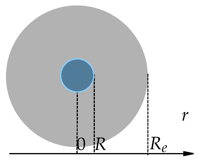
Figure 3.
Function for , , , and varying between V and V. The clinically interesting region occurs for .
Figure 3.
Function for , , , and varying between V and V. The clinically interesting region occurs for .
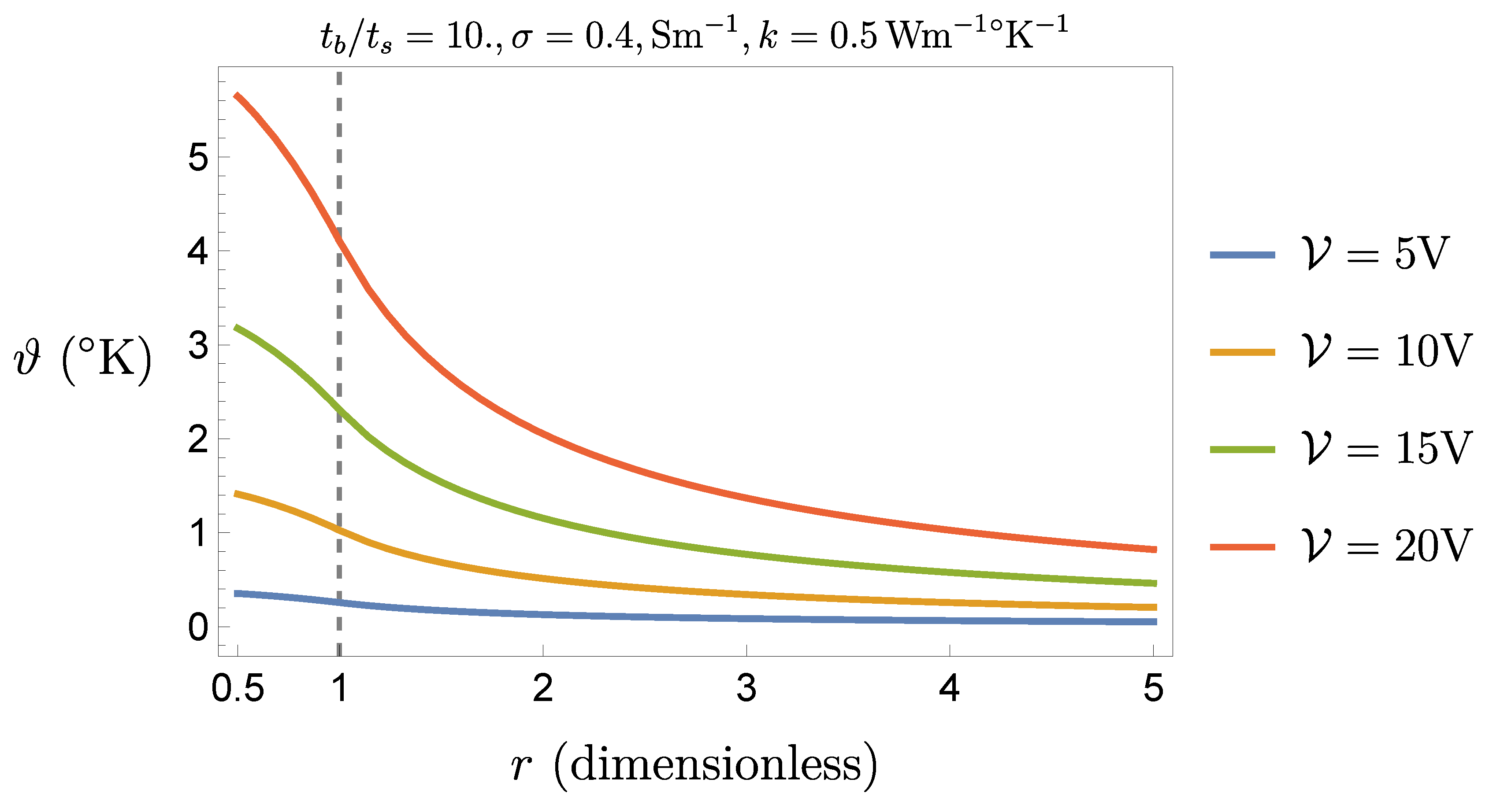
Figure 4.
Function for V, ,, and varying between 5 and 50. The clinically interesting region occurs for .
Figure 4.
Function for V, ,, and varying between 5 and 50. The clinically interesting region occurs for .
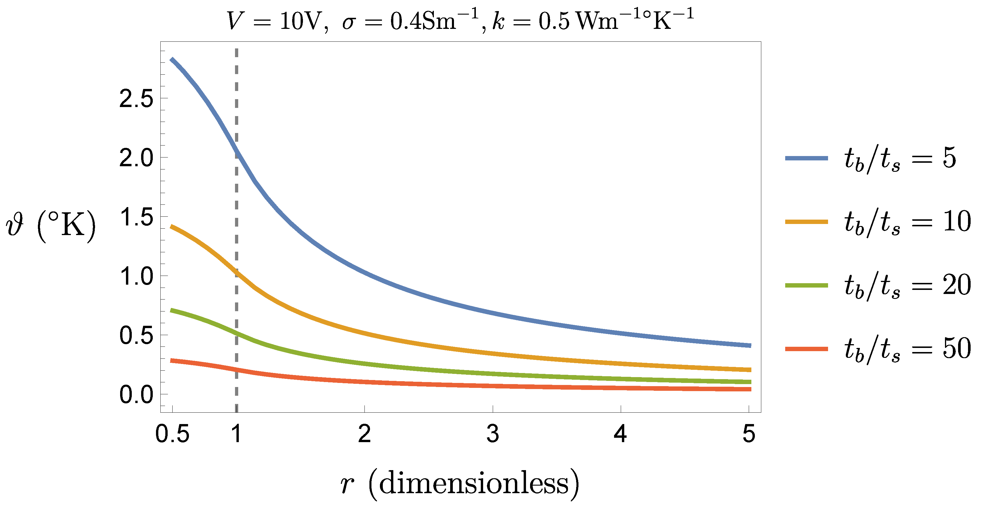
Figure 5.
Critical choice of when V (worst case) and , . Safety requires to maintain .
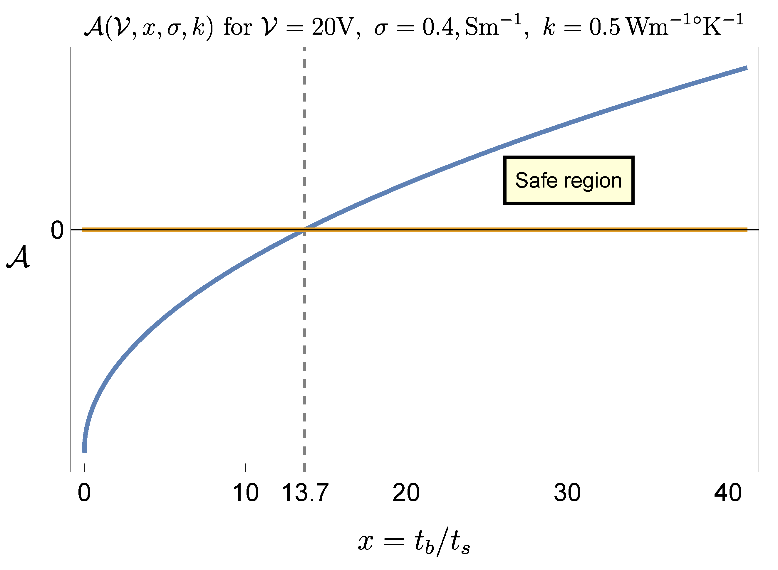
Figure 6.
Critical voltage when (worst case) and and , . Safety requires to maintain V.
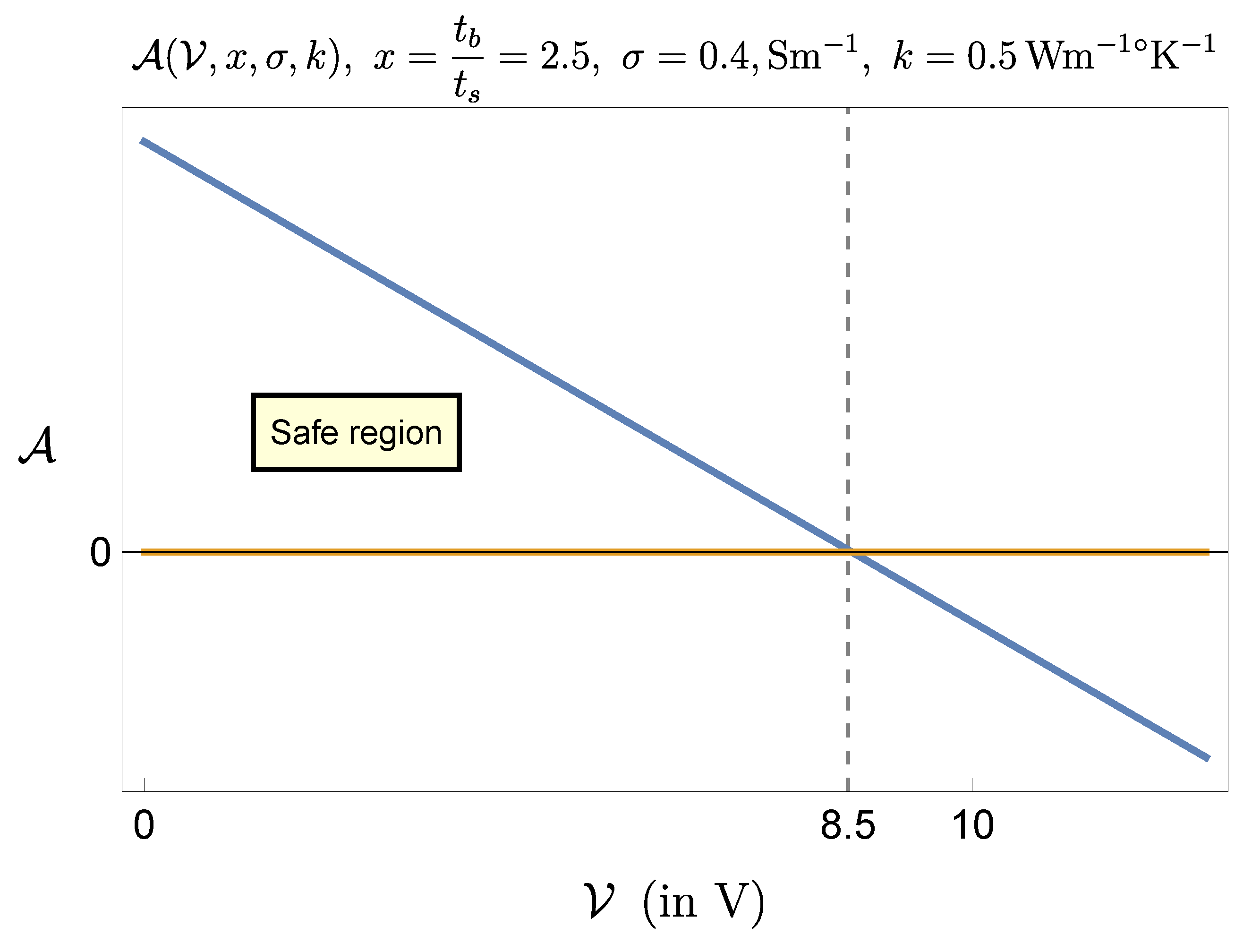
Figure 7.
The safety operating time ratio for and corresponds to .
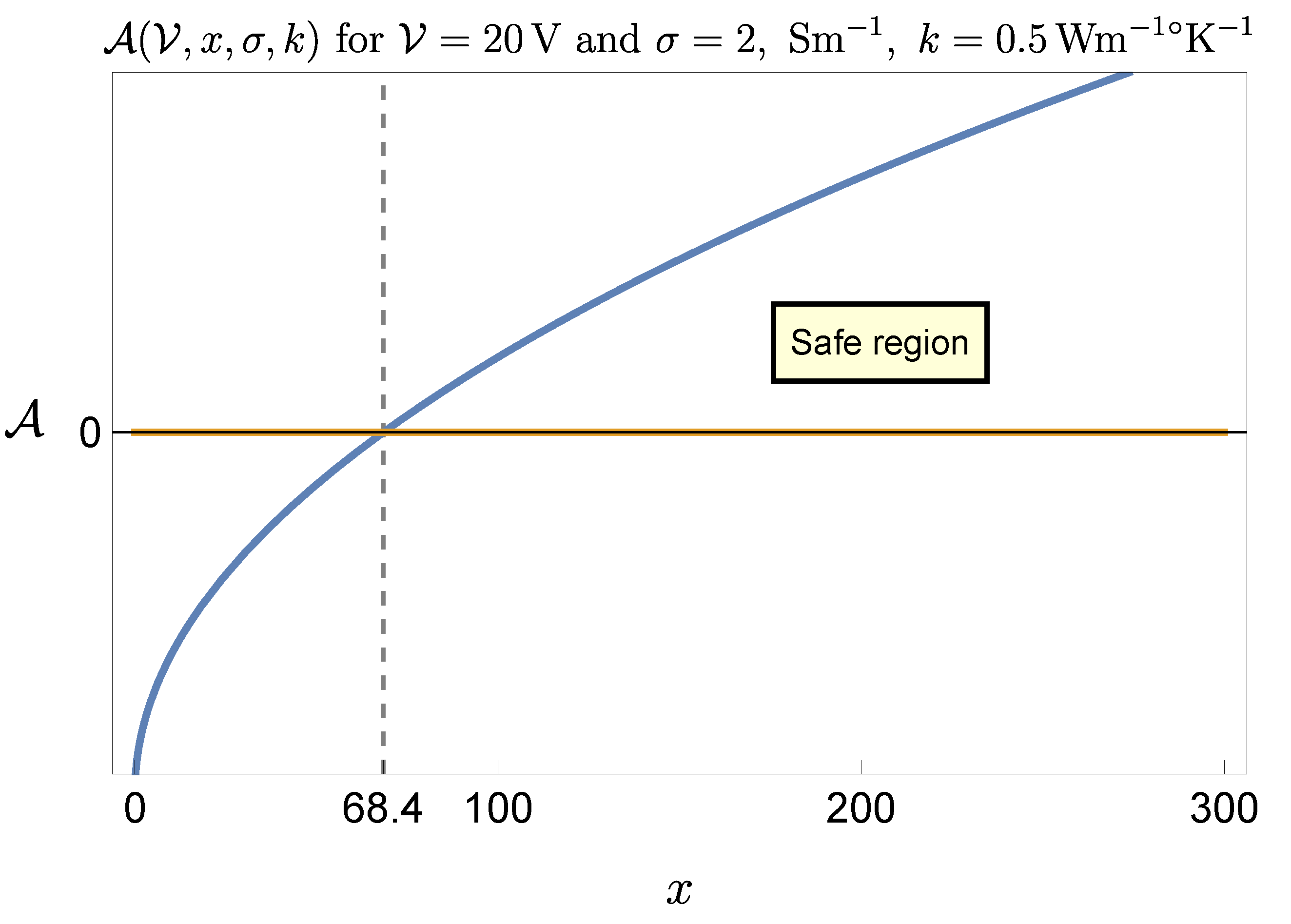
Figure 8.
The safety operating voltage for and corresponds to .
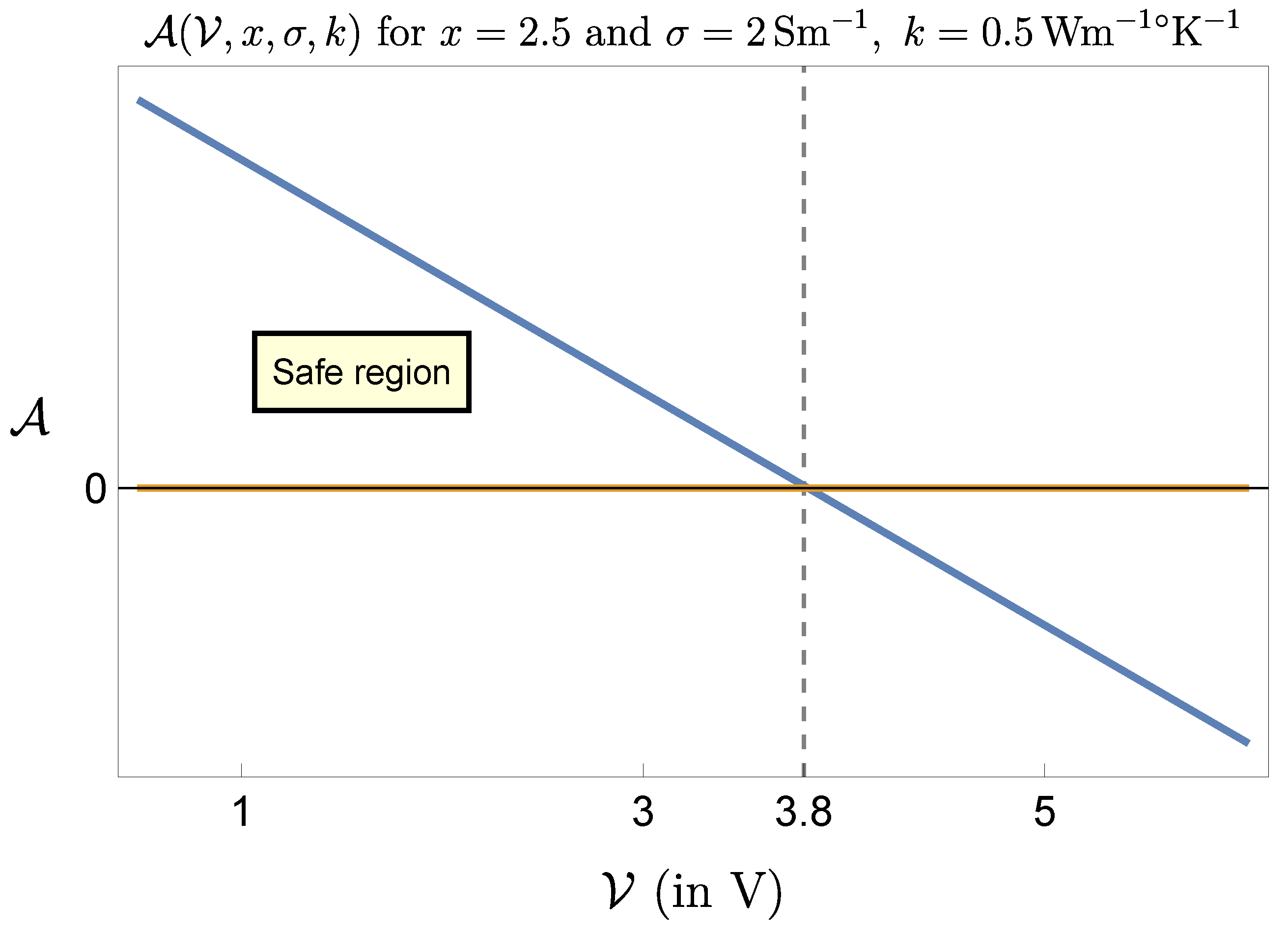
Figure 9.
Three-dimensional representation of the forbidden region where is negative (on the right panel) and three level sets of (on the left panel), when .
Figure 9.
Three-dimensional representation of the forbidden region where is negative (on the right panel) and three level sets of (on the left panel), when .
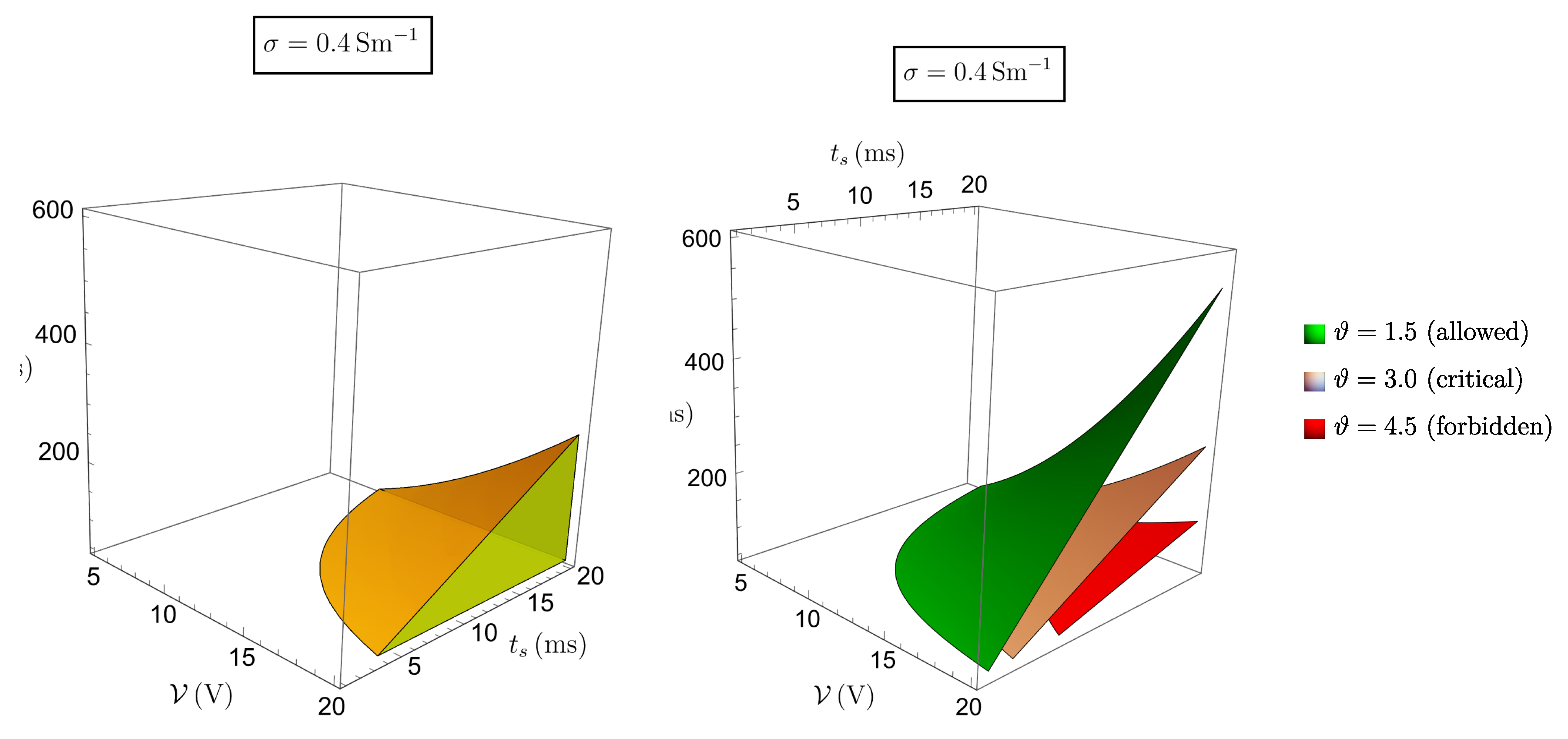
Figure 10.
Three-dimensional representation of the forbidden region where is negative (on the right panel) and three level sets of (on the left panel), when .
Figure 10.
Three-dimensional representation of the forbidden region where is negative (on the right panel) and three level sets of (on the left panel), when .
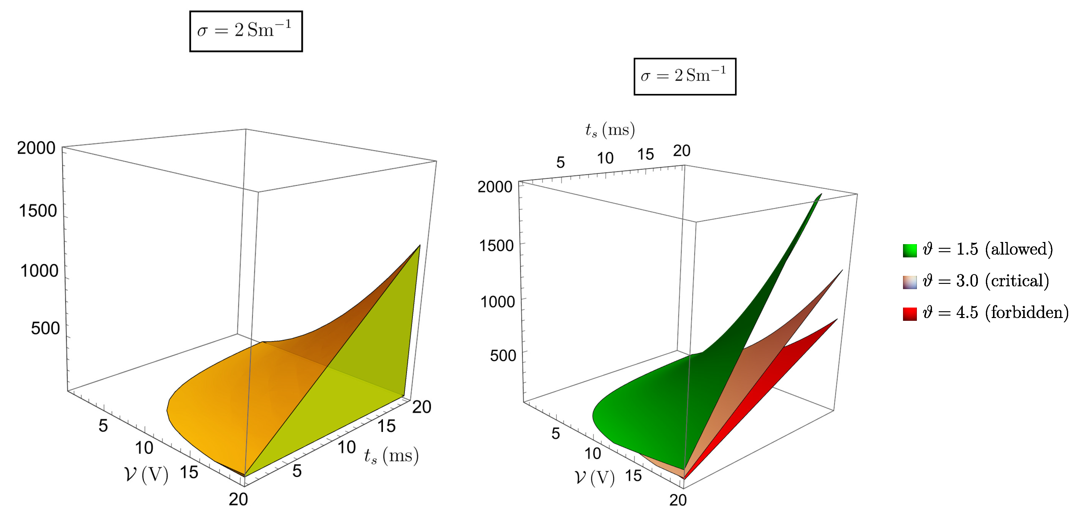
Figure 11.
The effect of heat removal due to blood perfusion compared with the case in which perfusion in not taken into account.
Figure 11.
The effect of heat removal due to blood perfusion compared with the case in which perfusion in not taken into account.
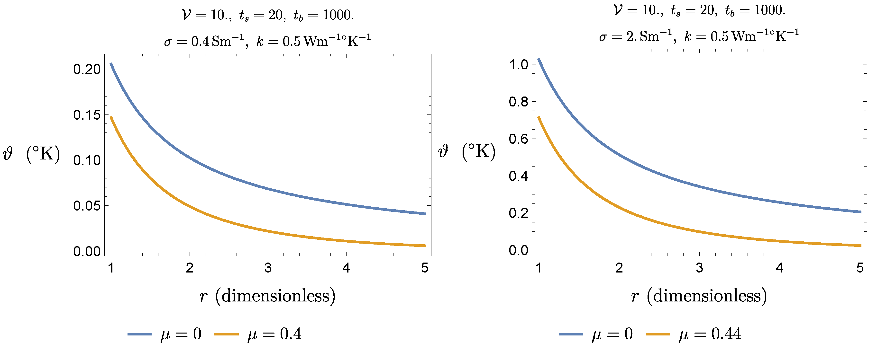
Figure 12.
Function shows the efficiency of perfusion in the area of interest.
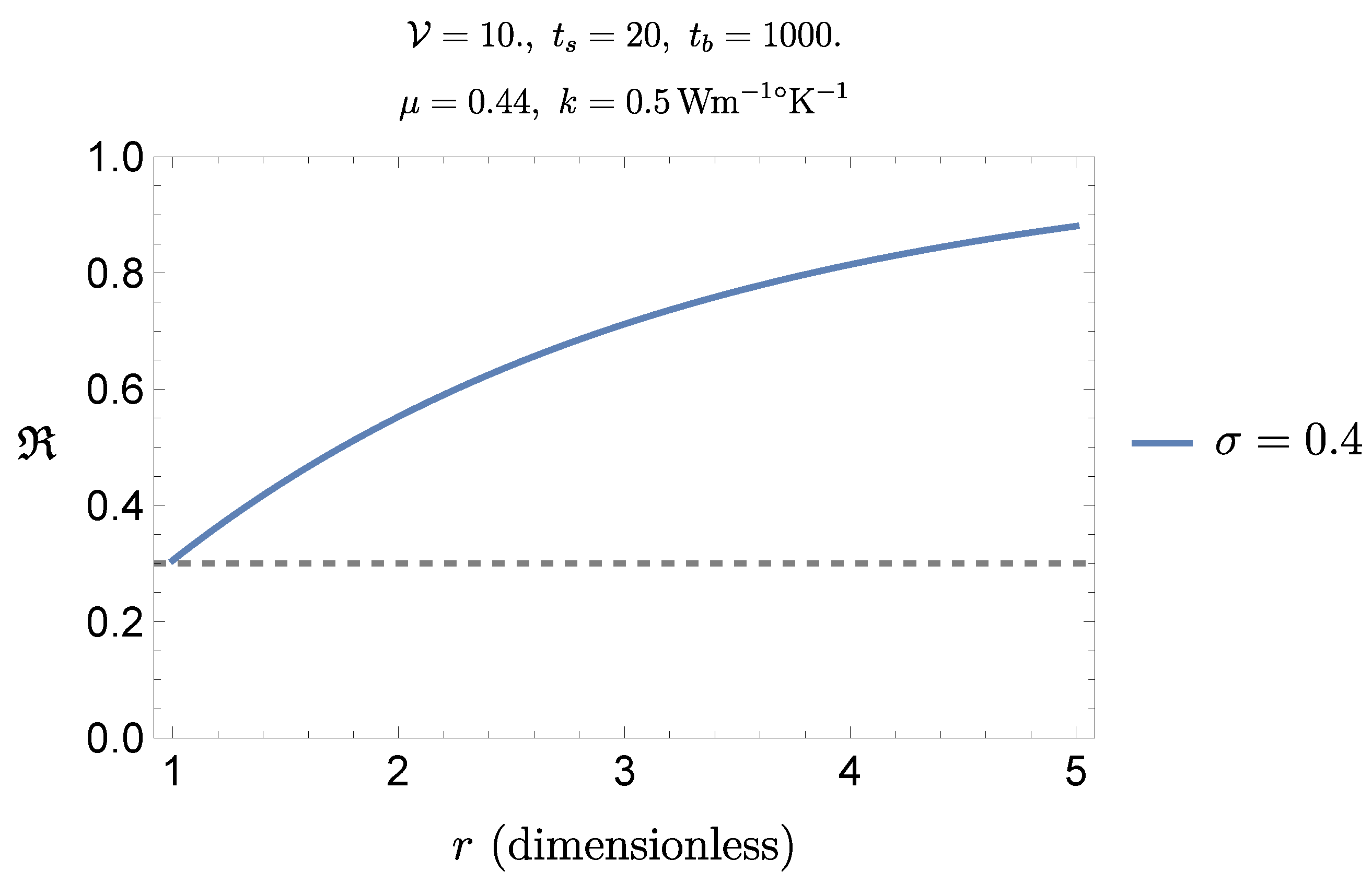
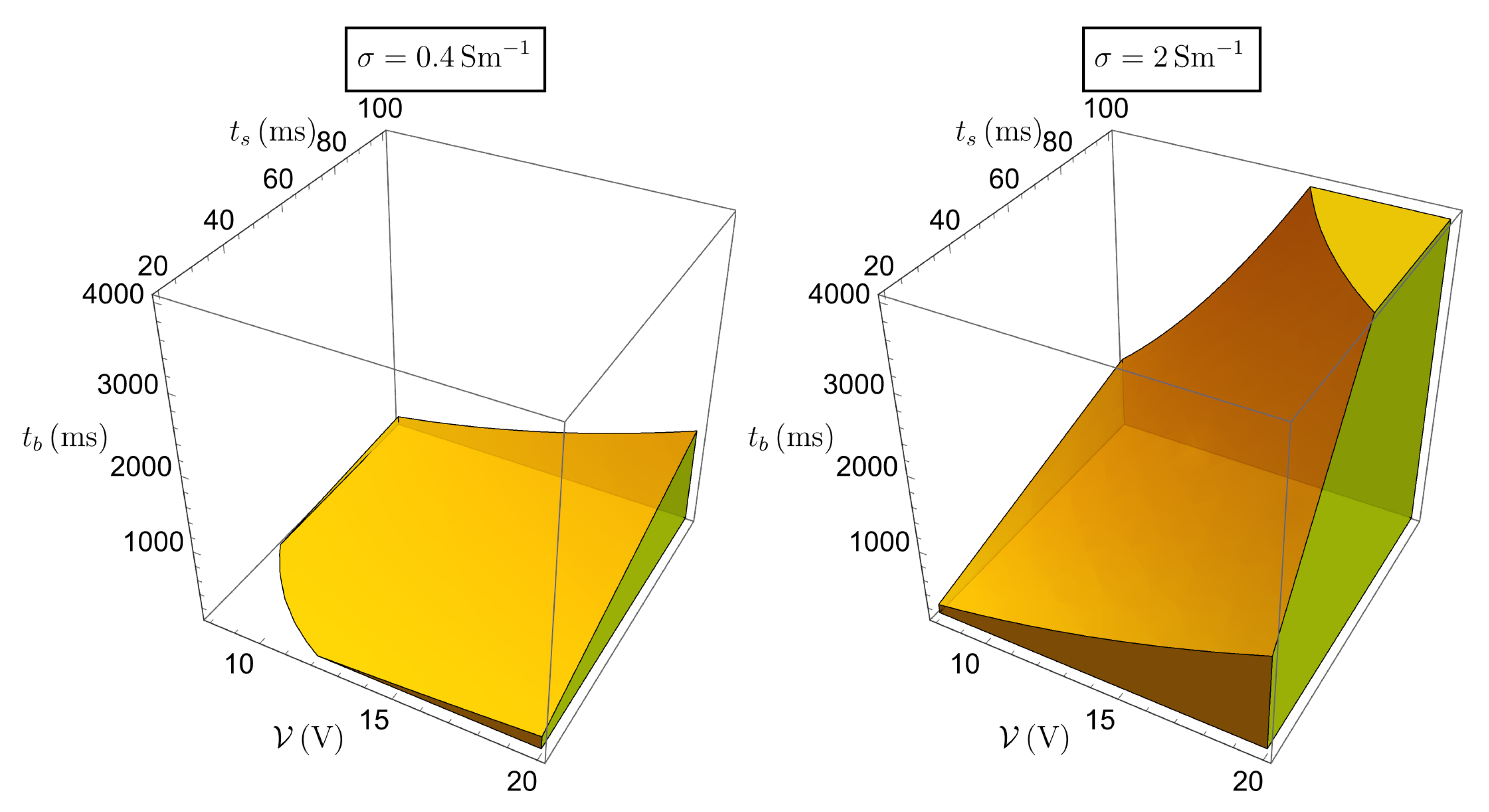
Figure 13.
Three-dimensional representation of the region of settable parameters which, although larger than the unsafe one shown In the lest panels of Figure 9 and Figure 10 (and so containing safe values of the parameters), has no efficacy from the therapeutic point of view. On the left side the case , on the right side the case .
Disclaimer/Publisher’s Note: The statements, opinions and data contained in all publications are solely those of the individual author(s) and contributor(s) and not of MDPI and/or the editor(s). MDPI and/or the editor(s) disclaim responsibility for any injury to people or property resulting from any ideas, methods, instructions or products referred to in the content. |
© 2024 by the authors. Licensee MDPI, Basel, Switzerland. This article is an open access article distributed under the terms and conditions of the Creative Commons Attribution (CC BY) license (http://creativecommons.org/licenses/by/4.0/).
Copyright: This open access article is published under a Creative Commons CC BY 4.0 license, which permit the free download, distribution, and reuse, provided that the author and preprint are cited in any reuse.


