Submitted:
13 August 2024
Posted:
14 August 2024
You are already at the latest version
Abstract
The increasing frequency and severity of phytoplankton blooms worldwide highlight the need for advancements in monitoring technologies. Optical remote sensors, such as Landsat, have proven to be a cost-effective method for large-scale, near-real-time assessments of phytoplankton biomass in lakes. However, its effectiveness is often compromised by atmospheric interferences like clouds, dust, and wildfire smoke, which can obscure the clear-sky conditions essential for accurate remote sensing. While partial atmospheric correction (removing only the Rayleigh effect) is commonly applied to address these interferences, it remains inadequate for mitigating the impact of wildfire smoke. This study investigates the potential of Landsat's coastal/aerosol band (B1) for assessing wildfire smoke interference effects on Chlorophyll-a (Chl-a) retrieval models, which serve as proxies for phytoplankton biomass. We employed cluster analysis of B1 values to create a screening system based on aerosol reflectance, categorizing smoke interference into low, moderate, and high levels. Subsequently, we applied both partial (Rayleigh-corrected reflectance) and full (Landsat 8 Level 2 surface reflectance) atmospheric corrections before developing the Chl-a retrieval models. Excluding high wildfire smoke interference (B1 > 0.07) from the Chl-a calibration dataset significantly enhanced model performance, increasing the r-squared value from approximately 0.55 to 0.80. Moderate smoke interference (0.05 < B1 < 0.07) yielded results comparable to low-interference conditions. Notably, Rayleigh-corrected reflectance, even without additional aerosol band filtering, achieved higher r-squared values for the Chl-a retrieval model than full atmospheric correction. B1 thus proves to be a valuable tool for identifying low smoke-impacted observations, offering an effective method to monitor phytoplankton biomass amid increasing wildfire activity and improving the capacity to monitor aquatic environments in a changing global landscape.
Keywords:
chlorophyll-a
; freshwater
; phytoplankton
; remote sensing
; wildfire
1. Introduction
Since the late 20th century, freshwater environments have experienced a troubling rise in phytoplankton blooms, marked by increasing frequency, intensity, and shifts in community composition [1]. Although phytoplankton populations typically exhibit seasonal patterns, anthropogenic stressors such as nutrient loading and climate change can disrupt these natural cycles, leading to harmful algal blooms [2,3]. These blooms degrade water quality, causing issues like toxin production, disruption of food webs, and anoxia, which in turn create substantial social, economic, and ecological challenges [4,5]. Given their responsiveness to environmental changes, phytoplankton are crucial indicators of water quality and are routinely monitored to assess the health of water bodies globally [6,7]. Developing tools to monitor phytoplankton dynamics within freshwater lakes is essential for enabling lake managers and practitioners to make informed decisions [8].
Chlorophyll-a (Chl-a) concentration, commonly used as a proxy for phytoplankton biomass [9], is measured through both field-based and remote sensing methods. Traditional field sampling provides high-resolution data at specific locations but lacks comprehensive spatial coverage and is resource-intensive [10,11]. The time-intensive nature of these methods can delay water management responses, which are critical for addressing phytoplankton-related threats [12]. In contrast, remote sensing offers a time-sensitive and cost-efficient technique for monitoring phytoplankton biomass across large areas [7,13,14,15,16,17,18,19]. This approach enables near-real-time, quantitative, and qualitative analyses of phytoplankton communities by capturing optical data on water bodies [17,20]. However, optical remote sensing is dependent on cloud-free and minimal atmospheric interference, as clouds, smoke, and haze can significantly degrade image quality [6,21].
One emerging concern is the increasing prevalence of wildfires, which produce smoke that obstructs remote sensing capabilities. Recent years have seen a global rise in wildfire frequency and intensity, exacerbated by climate change and historical fire suppression practices [22,23] (Figure 1a). For example, Canada experienced its worst wildfire season on record in 2023, with atmospheric carbon emissions four times higher than in previous years (Figure 1b). Wildfires not only impair water quality through ash deposition and light inhibition [23,24,25,26,27], but also degrade the quality of remote sensing images. Elevated aerosol levels can be partially mitigated through atmospheric correction in remote sensing products like Landsat Level 2 or Sentinel-2C [28,29]. However, for aquatic applications that often use partial atmospheric correction, wildfire smoke remains a challenge. Developing methodologies to classify and mitigate smoke effects in satellite imagery is crucial as wildfire activity increases globally. Such methodologies should enable the exclusion of smoke-impacted observations from analysis, thereby enhancing the reliability of water quality models in wildfire-affected areas.
This study utilizes the Landsat 8 coastal/aerosol band (B1) to categorize and quantify the level of wildfire smoke interference in remote sensing images. We assessed the impact of excluding varying degrees of smoke interference on the performance of Chl-a retrieval models. To validate our approach, we compared partially corrected reflectance data filtered by the aerosol band with fully corrected Landsat 8 Level 2 products. The results show that this methodology offers a reliable tool for mapping lake surface Chl-a, even in regions impacted by wildfires. This approach provides lake managers with a valuable tool for monitoring aquatic environments, establishing thresholds for wildfire interference, and ensuring the accuracy of remote sensing in an era of increasing wildfire activity.
2. Materials and Methods
2.1. Ground-Based Dataset
Chl-a samples were collected from 106 lakes within the Prairie Pothole Region of Canada, spanning Alberta, Saskatchewan, and Manitoba (Figure 2). Water samples were obtained using a 1-meter integrated sampler at the center or deepest point of each lake, as determined by bathymetric data. Phytoplankton samples were taken during the peak growing season, from mid-July to end of August [30,31]. To concentrate phytoplankton for Chl-a analysis, lake water was filtered through Whatman GF/F filters. The volume of water filtered ranged from 30 to 500 milliliters, depending on the algae concentration. The filters were then frozen at -20°C to preserve the pigments. Chl-a was extracted using 90% (v/v) acetone under dim light, and the filters were mechanically disrupted with a bead beater (3 × 10-second cycles) containing 0.1 mm zirconia/silica beads [32]. The mixture was stored at -20°C for 4 hours, followed by centrifugation (6,000 g for 5 minutes) for an initial clarification. The supernatant was further clarified by filtering through a 0.22 µm filter and then measured at 664 nm using a spectrophotometer (1 cm cuvette) following the Jeffrey and Humphrey method [33]. Chl-a concentrations were reported in µg L−1.
2.2. Landsat Image Acquisition, Processing, and Analysis
Data were acquired using the Landsat 8 Operational Land Imager (OLI), with the first six spectral bands extracted for each study lake (Table 1). Radiometric and atmospheric corrections were carried out using Google Earth Engine (GEE), a cloud-based platform that facilitates the processing of large geospatial datasets, including remote sensing data [34,35]. GEE has become a widely utilized tool for monitoring water quality in both inland and marine environments [36,37,38,39,40].
2.2.1. In Situ and Satellite Match Up Considerations
Ground-based Chl-a measurements were matched to corresponding satellite observations at the point of sampling within a temporal window of ± 1, 3, 7 days of satellite image capture. The selected temporal window was selected based on considerations of the sample size and the correlation between satellite band formula and in situ ln(Chl-a).
2.2.2. Atmospheric Correction
Atmospheric correction is essential for accurately mapping water optical properties, as it mitigates atmospheric interferences such as aerosol and Rayleigh scattering effects in satellite imagery [41,42]. Despite its importance, inland water research still lacks a standardized atmospheric correction algorithm [43,44]. Many studies (e.g., [17,44,45,46,47,48,49,50]) advocate for partial atmospheric correction—specifically removing Rayleigh scattering effects—because accurately estimating aerosol correction for water bodies is challenging and often results in overestimation of atmospheric radiance contributions.
In this study, partial atmospheric correction was performed as follows:
- Conversion to at-sensor spectral radiance: Landsat 8 OLI Level 1 data, comprising raw digital numbers (DN) ranging from 0 to 65,000, were used. Converting DN values to a common radiometric scale by calculating radiance is the first step in analyzing images from different sensors and platforms [51,52]. The DN values were converted to Top-of-Atmosphere (TOA) radiance using Equation (1) (Table 2; [51]).
- Calculation of Rayleigh scattering effects on at-sensor spectral radiance: To remove Rayleigh scattering from the TOA radiance, Equation (2) was applied (Table 2; [53]). The Rayleigh pressure (Pr) was calculated using Equation (3) (Table 2; [54,55]), Rayleigh optical thickness (τr) was determined using Equation (4) (Table 2; [53]), and ozone transmittance (τoz) was computed using Equation (5) (Table 2; [56,57]). Finally, Rayleigh-corrected TOA radiance (Lr) was obtained by subtracting it from Lλ using Equation (6) (Table 2).
- Conversion of Rayleigh-corrected radiances to partially-corrected BOA reflectance: The Rayleigh-corrected TOA radiance was then converted to Rayleigh-corrected Bottom-of-Atmosphere (BOA) reflectance (Rrc) using Equation (7) (Table 2), which was used to develop Chl-a retrieval models. This step offers multiple advantages: it eliminates the impact of varying solar zenith angles due to different image acquisition times, accounts for differences in Earth-Sun distances, and compensates for varying exoatmospheric solar irradiances [52].
2.3. Wildfire Correction
Wildfires are a frequent occurrence in Canada, but the 2023 wildfire season was unprecedented, marking the worst on record (Figure 1b). The resulting smoke significantly degraded the quality of satellite images. To quantify the extent of smoke interference, we used the Landsat coastal/aerosol band (B1 = 0.43-0.45 mm), which is particularly effective for monitoring atmospheric aerosol properties [58]. A k-means clustering approach (k = 3) was applied to the B1 data, allowing us to classify the lakes based on the severity of smoke interference into three categories: low (cluster 1), moderate (cluster 2), and high (cluster 3).
2.4. Chl-a Retrieval Model Development
For Chl-a retrieval model development, we used matchup results within a ± 3-day window. The blue (B2) and red (B4) bands were selected for their alignment with the maximum absorption of Chl-a, while the green band (B3) was chosen for its alignment with the maximum reflectance (i.e., minimal absorption) of Chl-a. These bands were incorporated into the development of band formulae to create a physically-based approach for Chl-a retrieval from remote sensing images. The performance of three band formulas—Blue/Green, Blue/Red, and (Blue-Red)/Green—was evaluated using 3-fold cross-validation. The Blue/Green [14,45] and Blue/Red [14,45,59,60] ratios are single-band formulas commonly used for mapping Chl-a in Landsat products. The third formula, (Blue-Red)/Green, has been widely adopted in Chl-a mapping on Landsat products (e.g., [17,19,59,61,62,63,64,65,66]).
2.5. Chl-a Retrieval Model Evaluation
To determine the optimal relationship between the band formulae and Chl-a, we employed 3-fold cross-validation. The 3-fold cross-validation process involves dividing the data into three sets for training and testing, enhancing the generalizability and predictive accuracy of the models. The performance of each model was assessed using multiple metrics, including the coefficient of determination (R²) (Equation (8); Table 2), Root Mean Square Error (RMSE) (Equation (9); Table 2), Normalized Root Mean Square Error (NRMSE) (Equation (10); Table 2), Mean Absolute Error (MAE) (Equation (11); Table 2), and Bias (Equation (12); Table 2).
3. Results
3.1. Landsat Image Acquisition, Processing, and Analysis
The selected temporal window for matchups between ground-based Chl-a measurements and corresponding satellite observations at the point of sampling was ± 3 days of satellite image capture (Figure 3). This temporal window achieved a balance between sample size and the correlation between satellite band formula and in situ ln(Chl-a). The ± 1 day had the smallest number of samples but the highest correlation with in situ ln(Chl-a), while the ± 7 days had the largest number of samples but a marginally smaller correlation with in situ ln(Chl-a) compared to ± 3 days.
3.2. Clustering the Impact of Wildfires on Remote Sensing Imagery
To assess wildfire effects on remote sensing imagery, B1 values at the in-situ sampling locations were extracted and subjected to k-means clustering analysis (k = 3) (Figure 4). The first cluster comprised samples with low aerosol band values (B1 < 0.05, Rrc), indicating minimal interference. The second cluster represented lakes with moderate aerosol levels (0.05 ≤ B1 ≤ 0.07, Rrc), while the third cluster consisted of observations with high aerosol levels (B1 > 0.07, Rrc). The significance of differences between these clusters was evaluated using the Kruskal-Wallis test, a nonparametric method that compares the mean ranks across clusters. The results indicated that the clusters were statistically distinct (p < 0.001).
3.3. Performance of Chl-a Retrieval Models with Partial Atmospheric Correction
To investigate the impact of incorporating samples with varying aerosol band values into the Chl-a retrieval model, three calibration datasets were established:
- Calibration set 1: Includes cluster 1 (low wildfire interference).
- Calibration set 2: Includes clusters 1 and 2 (low and moderate wildfire interference).
- Calibration set 3: Includes all clusters (low, moderate, and high wildfire interference).
A 3-fold cross-validation method was applied, and Table 3, section A presents the performance metrics of the best fold based on the test fold. It outlines the performance of models developed using three predictors across different calibration sets. Calibration set 1 consistently outperformed the other sets in terms of all predictors’ performance metrics. Specifically, models based on (Blue-Red)/Green exhibited superior R² and NRMSE compared to the other predictors across all calibration sets. Calibration set 2 showed slightly lower performance than set 1 across all predictors, while Calibration set 3 exhibited the weakest performance among all calibration sets.
3.4. Performance of Chl-a Retrieval Models with Full Atmospheric Correction
To assess whether Chl-a retrieval models developed with partial atmospheric correction are comparable to those with full atmospheric correction, Landsat 8 level 2 (process-ready) products were utilized. A calibration dataset incorporating both in-situ and satellite overpass data, with a match-up window size limited to +/- 3 days, was employed. Table 3, section B presents the performance metrics of Chl-a retrieval modeling using Landsat level 2 products for different calibration sets. Calibration set 1 demonstrated superior performance across all predictors compared to other calibration sets. Models based on (Blue-Red)/Green showed the highest R² and NRMSE values for Calibration sets 1 and 2. Calibration set 3 consistently exhibited the weakest performance among all calibration sets.
3.5. Comparison of Chl-a Retrieval Modeling
Figure 5a illustrates the performance of different band formulas on the Rayleigh-corrected reflectance dataset. Calibration set 1 achieved the highest R² values among all calibration sets. Calibration set 2 showed a slight decline in performance across all models, although a two-way ANOVA test indicated no statistically significant difference in R² values between calibration sets 1 and 2 (p > 0.1). Calibration set 3 consistently demonstrated lower performance compared to sets 1 and 2, with ANOVA results confirming significant differences in mean R² values (p < 0.01).
Figure 5b depicts the performance of different band formulas on the surface reflectance product. Similarly, ANOVA tests revealed that Calibration set 1 significantly outperformed both calibration sets 2 and 3 (p < 0.001), while the performance difference between Calibration sets 2 and 3 was not statistically significant (p = 0.2). Within each calibration set, there were no significant differences in the performance of each band formula (p > 0.1).
Observations in Calibration set 1 for both Rayleigh-corrected reflectance (Figure 5a) and Landsat level 2 products (Figure 4b) indicated minimal aerosol disturbance. Comparing these two calibration sets highlighted the impact of aerosol effects on Chl-a retrieval modeling in surface waters. Specifically, the full atmospheric correction used in the Landsat level 2 product (Figure 5b - Calibration set 1) underperformed compared to partial atmospheric correction (Figure 5a - Calibration set 1), with R² values decreasing by approximately 0.1.
The two-way ANOVA showed that the (a) Rayleigh-corrected reflectance and (b) Landsat level 2 calibration sets between both products were statistically different across all three calibration sets (p < 0.001).
3.6. Effect of Aerosol Band Filtering on Lake Chl-a Concentrations Across the Lake Winnipeg Watershed
To assess the impact of using aerosol band filtering for removing pixels with elevated aerosol levels in the process of mapping lake Chl-a concentrations, we employed a model based on the (Blue-Red)/Green band formula. This model was used to map phytoplankton biomass (i.e., Chl-a concentration) across lakes in the Lake Winnipeg Watershed from 2013 to 2023. The formula was derived from Calibration set 2, which utilized Rayleigh-corrected reflectance. While Calibration set 2 did not achieve the highest performance among all sets (R² = 0.83), its performance was only slightly lower than that of Calibration set 1 (R² = 0.80), with no statistically significant difference between the two. Notably, Calibration set 2 included nearly twice as many samples as Calibration set 1 (17 versus 9), thus providing a more extensive dataset for model development. Figure 6a maps the differences in average Chl-a concentration for each lake between 2013 and 2023, with and without aerosol band filtering. Figures 6b and c show the frequency distributions of lake Chl-a concentrations, comparing the scenarios without and with aerosol filtering for the average Chl-a concentration between 2013 to 2023.
4. Discussion
The increasing frequency and intensity of wildfires highlight the need for advanced monitoring techniques to address the challenges posed by heightened haze and smoke levels on remote sensing methods [67]. Elevated haze and smoke from wildfires reduce visibility and degrade satellite imagery quality [68,69], making it difficult to extract reliable information about surface properties, such as water quality characteristics [21,70,71]. Lake managers and practitioners need guidance on whether image quality is sufficient for accurately characterizing algal dynamics.
4.1. Removing Effects of Severe Smoke
In this study, we applied a three-tiered image categorization system based on aerosol band values to assess smoke severity. We found that including samples with higher aerosol band values (i.e., higher smoke levels) in the calibration dataset led to a continuous decline in model performance, as indicated by decreasing R² values for all band formulae. When aerosol band values exceeded a threshold of 0.07 (Rrc, unitless), the accuracy of the Chl-a model was significantly affected, and such observations should be excluded to avoid inaccuracies. Nevertheless, even with highly smoke-affected observations (cluster 3), the models achieved R² values around 0.55 (Table 3, section A, Calibration set 3), which is still considered acceptable in previous studies using Landsat 8 OLI (e.g., [63,72,73]).
Our long-term and large-scale analysis of the effects of aerosol band filtering on pixel selection for Chl-a mapping (Figure 6a) showed that, for most monitored lakes in the Lake Winnipeg Watershed between 2013 and 2023, the observed differences between including and excluding this filter were relatively small (between -5 to 5 µg/L), indicating similar results. However, for some lakes, the observed differences exceeded 5 µg/L. Additionally, Figure 6b shows that for phytoplankton-rich lakes with Chl-a concentrations over 53 µg/L (or ln(Chl-a) > 4), both methods produced similar frequency distributions of lakes. In contrast, for lakes with Chl-a concentrations below 53 µg/L, the differences between the two methods were more pronounced. Specifically, for ln(Chl-a) values below 2.5 (equal to 12 µg/L), implementing aerosol band filtering mapped more lakes than without the filter, while in the range of ln(Chl-a) between 2.5 and 4, excluding aerosol filtering resulted in mapping more lakes.
A growing number of researchers are relying on Rayleigh-corrected reflectance, which remains vulnerable to smoke interference from wildfires [74]. This underscores the need for continued research into correction algorithms that can accurately account for elevated aerosol levels from wildfires across diverse surface types. Filtering Rayleigh-corrected reflectance with the coastal/aerosol band can be useful for detecting and excluding observations with high levels of smoke in the remote sensing of water bodies. Moreover, we found that full atmospheric correction, commonly used in previous studies, is often ineffective at removing wildfire effects and can impair model performance. This underperformance may be due to the overestimation of aerosol contributions, as documented in the literature [46,75].
4.2. Evaluating Chl-a retrieval Model Performance after Removal of Smoke Effects
The study area, covering the prairie and boreal plain ecozones, spans a wide range of lake productivity, from oligotrophic to eutrophic conditions [28]. In the southern prairie ecozone, lakes are often eutrophic due to the region’s phosphorus-rich geology together with intensive human activity. In contrast, the northern boreal plain ecozone, lakes are often oligotrophic due to minimal human activity [31]. Our study lakes exhibited a varied range of phytoplankton biomass, from 3.7 to 216 µg/L of Chl-a (Table S1).
All three band combinations used for Chl-a retrieval showed high performance (R² > 0.78) when using Calibration sets 1 and 2. Regardless of the band combination, Calibration set 3 performed poorly (R² < 0.58), illustrating the negative impact of high wildfire smoke on model performance. The (Blue-Red)/Green ratio exhibited the best performance in modeling Chl-a across all three calibration sets. This band formula has been widely used for mapping Chl-a in various water bodies (e.g., [19,59,62,63]) and is known for its broad applicability, effectively tracking Chl-a across different trophic states [17,62].
A key consideration when applying the (Blue-Red)/Green ratio is its susceptibility to high chromophoric dissolved organic matter (CDOM). High CDOM can limit the effectiveness of this method, as CDOM interferes with phytoplankton detection in the blue spectrum [64]. However, our study lakes had relatively low color (<65 mg/L PtCo), supporting the suitability of this method in our analysis (Table S1).
4. Conclusion
As wildfires become more frequent and intense worldwide, the resulting smoke plumes can travel hundreds to thousands of kilometers, posing significant challenges to the accuracy of satellite sensor data, which is crucial for monitoring freshwater lakes. To maintain precision in water quality assessments under these wildfire-affected conditions, it is essential to implement tailored strategies, such as refined atmospheric corrections and well-defined cutoff thresholds. In this study, we identified a specific threshold at which wildfire smoke significantly impairs the prediction of algal productivity. By integrating this threshold with Rayleigh-corrected reflectance, we effectively assessed lakes impacted by wildfire smoke. This highlights the need for remote sensing practitioners to recognize when predictive accuracy is compromised, ensuring more reliable monitoring and assessment of wildfire-affected regions.
Author Contributions
In this research, author’s contribution is presented as: Conceptualization, S.M. and I.F.C; methodology, S.M. and K.J.E.; software, S.M.; validation, S.M., I.F.C and K.J.E.; formal analysis, S.M.; investigation, S.M. and I.F.C; resources, I.F.C.; data curation, S.M. and K.J.E.; writing—original draft preparation, S.M.; writing—review and editing, S.M., I.F.C. and K.J.E.; visualization, S.M. and K.J.E; supervision, I.F.C.; project administration, I.F.C.; funding acquisition, I.F.C. All authors have read and agreed to the published version of the manuscript.
Funding
The research was funded by a Natural Sciences and Engineering Research Council of Canada (NSERC) Discovery Grant (05265-2019) and an Environment and Climate Change Canada - Climate Action and Awareness Fund (ECCC-CAAF) (EDF-CA-2021i023) grant awarded to I.F.C.
Data Availability Statement
This research has used Landsat OLI images, openly available in the Google Earth Engine (https://earthengine.google.com/) platform. The raw chlorophyll-a data supporting the conclusions of this article will be made available by the authors on request.
Acknowledgments
The authors wish to thank David Aldred and Michael Dallosch for their technical support.
Conflicts of Interest
The authors declare no conflicts of interest.
References
- Downing, J.A. Limnology and oceanography: two estranged twins reuniting by global change. Inland waters 2014, 4, 215–232. [Google Scholar] [CrossRef]
- Paerl, H.W.; Huisman, J. Blooms like it hot. Science 2008, 320, 57–58. [Google Scholar] [CrossRef]
- Wurtsbaugh, W.A.; Paerl, H.W.; Dodds, W.K. Nutrients, eutrophication and harmful algal blooms along the freshwater to marine continuum. Wiley Interdiscip. Rev.-Water 2019, 6, e1373. [Google Scholar] [CrossRef]
- Brooks, B.W.; Lazorchak, J.M.; Howard, M.D.; Johnson, M.V.V.; Morton, S.L.; Perkins, D.A.; Reavie, E.D.; Scott, G.I.; Smith, S.A.; Steevens, J.A. Are harmful algal blooms becoming the greatest inland water quality threat to public health and aquatic ecosystems? Environ. Toxicol. Chem. 2016, 35, 6–13. [Google Scholar] [CrossRef] [PubMed]
- Chorus, I.; Fastner, J.; Welker, M. Cyanobacteria and cyanotoxins in a changing environment: Concepts, controversies, challenges. Water, 2021, 13, 2463. [Google Scholar] [CrossRef]
- Dörnhöfer, K.; Klinger, P.; Heege, T.; Oppelt, N. Multi-sensor satellite and in situ monitoring of phytoplankton development in a eutrophic-mesotrophic lake. Sci. Total Environ. 2018, 612, 1200–1214. [Google Scholar] [CrossRef]
- Sòria-Perpinyà, X.; Vicente, E.; Urrego, P.; Pereira-Sandoval, M.; Ruíz-Verdú, A.; Delegido, J.; Soria, J.M.; Moreno, J. Remote sensing of cyanobacterial blooms in a hypertrophic lagoon (Albufera of València, Eastern Iberian Peninsula) using multitemporal Sentinel-2 images. Sci. Total Environ. 2020, 698, 134305. [Google Scholar] [CrossRef]
- Mishra, S.; Stumpf, R.P.; Schaeffer, B.A.; Werdell, P.J.; Loftin, K.A.; Meredith, A. Measurement of cyanobacterial bloom magnitude using satellite remote sensing. Sci. Rep. 2019, 9, 1–17. [Google Scholar] [CrossRef]
- Boyer, J.N.; Kelble, C.R.; Ortner, P.B.; Rudnick, D.T. Phytoplankton bloom status: Chlorophyll a biomass as an indicator of water quality condition in the southern estuaries of Florida, USA. Ecol. Indic. 2009, 9, 56–67. [Google Scholar] [CrossRef]
- Olmanson, L.G. , Brezonik, P.L., Bauer, M.E. Remote sensing for regional lake water quality assessment: capabilities and limitations of current and upcoming satellite systems. In Advances in Watershed Science and Assessment, Younos, T., Parece, T., Eds.; Springer International Publishing, Switzerland, 2015; The Handbook of Environmental Chemistry 33, pp. 111– 140. [CrossRef]
- Papenfus, M.; Schaeffer, B.; Pollard, A.I.; Loftin, K. Exploring the potential value of satellite remote sensing to monitor chlorophyll-a for US lakes and reservoirs. Environ. Monit. Assess. 2020, 192, 808. [Google Scholar] [CrossRef] [PubMed]
- Randolph, K.; Wilson, J.; Tedesco, L.; Li, L.; Pascual, D.L.; Soyeux, E. Hyperspectral remote sensing of cyanobacteria in turbid productive water using optically active pigments, chlorophyll a and phycocyanin. Remote Sens. Environ. 2008, 112, 4009–4019. [Google Scholar] [CrossRef]
- Binding, C.E.; Greenberg, T.A.; McCullough, G.; Watson, S.B.; Page, E. An analysis of satellite-derived chlorophyll and algal bloom indices on Lake Winnipeg. J. Gt. Lakes Res. 2018, 44, 436–446. [Google Scholar] [CrossRef]
- Brezonik, P.; Menken, K.D.; Bauer, M. Landsat-based remote sensing of lake water quality characteristics, including chlorophyll and colored dissolved organic matter (CDOM). Lake Reserv. Manag. 2005, 21, 373–382. [Google Scholar] [CrossRef]
- Hou, X.; Feng, L.; Dai, Y.; Hu, C.; Gibson, L.; Tang, J.; Lee, Z.; Wang, Y.; Cai, X.; Liu, J.; Zheng, Y.; Zheng, C. Global mapping reveals increase in lacustrine algal blooms over the past decade. Nat. Geosci. 2022, 15, 130–134. [Google Scholar] [CrossRef]
- Palmer, S.C.J.; Kutser, T.; Hunter, P.D. Remote sensing of inland waters: Challenges, progress, and future directions. Remote Sens. Environ. 2015, 157, 1–8. [Google Scholar] [CrossRef]
- Paltsev, A.; Creed, I.F. Are northern lakes in relatively intact temperate forests showing signs of increasing phytoplankton biomass? Ecosystems 2022, 25. [Google Scholar] [CrossRef]
- Paltsev, A.; Creed, I.F. Multi-decadal changes in phytoplankton biomass in northern temperate lakes as seen through the prism of landscape properties. Glob. Change Biol. 2022, 28, 2272–2285. [Google Scholar] [CrossRef] [PubMed]
- Tan, W.; Liu, P.; Liu, Y.; Yang, S.; Feng, S. A 30-year assessment of phytoplankton blooms in Erhai lake using Landsat imagery: 1987 to 2016. Remote Sens. 2017, 9, 1265. [Google Scholar] [CrossRef]
- Sass, G.Z.; Creed, I.F.; Bayley, S.E.; Devito, K.J. Understanding variation in trophic status of lakes on the Boreal Plain: A 20-year retrospective using Landsat TM imagery. Remote Sens. Environ. 2007, 109, 127–141. [Google Scholar] [CrossRef]
- Hong, G.; Zhang, Y. Haze removal for new generation optical sensors. Int. J. Remote Sens. 2018, 39, 1491–1509. [Google Scholar] [CrossRef]
- Pinardi, M.; Stroppiana, D.; Caroni, R.; Parigi, L.; Tellina, G.; Free, G.; Giardino, C.; Albergel, C.; Bresciani, M. Assessing the impact of wild fires on water quality using satellite remote sensing: The Lake Baikal case study. Front. Remote Sens. 2023, 4, 1107275. [Google Scholar] [CrossRef]
- Raoelison, O.D.; Valenca, R.; Lee, A.; Karim, S.; Webster, J.P.; Poulin, B.A.; Mohanty, S.K. Wildfire impacts on surface water quality parameters: Cause of data variability and reporting needs. Environ. Pollut. 2023, 317, 120713. [Google Scholar] [CrossRef]
- Murphy, S.F.; Alpers, C.N.; Anderson, C.W.; Banta, J.R.; Blake, J.M.; Carpenter, K.D.; Clark, G.D.; Clow, D.W.; Hempel, L.A.; Martin, D.A.; Meador, M.R.; Mendez, G.O.; Mueller-solger, A.B.; Stewart, M.A.; Payne, S.E.; Peterman, C.L.; Ebel, B.A. A call for strategic water-quality monitoring to advance assessment and prediction of wildfire impacts on water supplies. Front. Water. 2023, 5, 1144225. [Google Scholar] [CrossRef]
- Paul, M.J.; Leduc, S.D.; Lassiter, M.G.; Moorhead, L.C.; Noyes, P.D.; Leibowitz, S.G. Wildfire induces changes in receiving waters: A review with considerations for water quality management. Water Resour Res. 2022, 58, 1–28. [Google Scholar] [CrossRef]
- Robinne, F.; Miller, C.; Parisien, M.; Emelko, M.B.; Bladon, K.D.; Silins, U.; Flannigan, M. A global index for mapping the exposure of water resources to wildfire. Forests 2016, 7, 22. [Google Scholar] [CrossRef]
- Williams, A.P.; Livneh, B.; McKinnon, K.A.; Hansen, W.D.; Mankin, J.S.; Cook, B.I.; Smerdon, J.E.; Varuolo-Clarke, A.M.; Bjarke, N.R.; Juang, C.S.; Lettenmaier, D.P. Growing impact of wildfire on western US water supply. PNAS 2022, 119, e2114069119. [Google Scholar] [CrossRef]
- Kganyago, M.; Ovakoglou, G.; Mhangara, P.; Alexandridis, T.; Odindi, J.; Adjorlolo, C.; Mashiyi, N. Validation of atmospheric correction approaches for Sentinel-2 under partly-cloudy conditions in an African agricultural landscape. In Remote Sensing of Clouds and the Atmosphere XXV, Proceedings of SPIE Vol, 11531(115310B), 1–19, 21-25 September 2020. [CrossRef]
- Pinto, C.T.; Jing, X.; Leigh, L. Evaluation analysis of Landsat Level-1 and Level-2 data products using in situ measurements. Remote Sens. 2020, 12, 2597. [Google Scholar] [CrossRef]
- Hayes, N.M.; Haig, H.A.; Simpson, G.L.; Leavitt, P.R. Effects of lake warming on the seasonal risk of toxic cyanobacteria exposure. Limnol. Oceanogr. Lett. 2020, 5, 393–402. [Google Scholar] [CrossRef]
- Mackeigan, P.W.; Taranu, E.; Pick, F.R.; Beisner, B.E.; Gregory-eaves, I. Both biotic and abiotic predictors explain significant variation in cyanobacteria biomass across lakes from temperate to subarctic zones. Limnol. Oceanogr. 2023, 68, 1360–1375. [Google Scholar] [CrossRef]
- Erratt, K.J.; Creed, I.F.; Trick, C.G. Comparative effects of ammonium, nitrate and urea on growth and photosynthetic efficiency of three bloom-forming cyanobacteria. Freshw. Biol. 2018, 63, 626–638. [Google Scholar] [CrossRef]
- Jeffrey, S.W.; Humphrey, G.F. New spectrophotometric equations for determining chlorophylls a, b, c1 and c2 in higher plants, algae and natural phytoplankton. Biochemie Und Physiologie Der Pflanzen, 1975, 167, 191–194. [Google Scholar] [CrossRef]
- Gorelick, N.; Hancher, M.; Dixon, M.; Ilyushchenko, S.; Thau, D.; Moore, R. Google Earth Engine : Planetary-scale geospatial analysis for everyone. Remote Sens. Environ. 2017, 202, 18–27. [Google Scholar] [CrossRef]
- Velastegui-Montoya, A.; Montalván-Burbano, N.; Carrión-Mero, P.; Rivera-Torres, H.; Sadeck, L.; Adami, M.G. Google Earth Engine: A global analysis and future trends. Remote Sens. 2023, 15, 3675. [Google Scholar] [CrossRef]
- Chu, H.; He, Y.; Nisa, W.; Jaelani, L.M. Multi-reservoir water quality mapping from remote sensing using spatial regression. Sustainability, 2021, 13, 6416. [Google Scholar] [CrossRef]
- Jin, H.; And, S.F.; Chen, C. Mapping of the spatial scope and water quality of surface water based on the Google Earth Engine cloud platform and Landsat time series. Remote Sens. 2023, 15, 4986. [Google Scholar] [CrossRef]
- Katlane, R.; El, B.; Dhaoui, O.; Kateb, F.; Chehata, N. Monitoring of sea surface temperature, chlorophyll, and turbidity in Tunisian waters from 2005 to 2020 using MODIS imagery and the Google Earth Engine. Reg. Stud. Mar. Sci. 2023, 66, 103143. [Google Scholar] [CrossRef]
- Kwong, I.H.Y.; Wong, F.K.K.; Fung, T. Automatic mapping and monitoring of marine water quality parameters in Hong Kong using Sentinel-2 image time-series and Google Earth Engine cloud computing. Front. Mar. Sci. 2022, 9, 871470. [Google Scholar] [CrossRef]
- Sagan, V.; Peterson, K.T.; Maimaitijiang, M.; Sidike, P.; Sloan, J.; Greeling, B.A.; Maalouf, S. ; Adams, Monitoring inland water quality using remote sensing: Potential and limitations of spectral indices, bio-optical simulations, machine learning, and cloud computing. Earth-Sci. Rev. 2020, 205, 103187. [Google Scholar] [CrossRef]
- Bresciani, M.; Cazzaniga, I.; Austoni, M.; Sforzi, T.; Buzzi, F.; Morabito, G.; Giardino, C. Mapping phytoplankton blooms in deep subalpine lakes from Sentinel-2A and Landsat-8. Hydrobiologia, 2018, 824, 197–214. [Google Scholar] [CrossRef]
- Katsoulis-dimitriou, S.; Lefkaditis, M.; Barmpagiannakos, S. Comparison of iCOR and Rayleigh atmospheric correction methods on Sentinel-3 OLCI images for a shallow eutrophic reservoir. PeerJ , 2022, 10, e14311. [Google Scholar] [CrossRef]
- Kuhn, C.; de Matos Valerio, A.; Ward, N.; Loken, L.; Sawakuchi, H.O.; Kampel, M.; Richey, J.; Stadler, P.; Crawford, J.; Striegl, R.; Vermote, E.; Pahlevan, N.; Butman, D. Performance of Landsat-8 and Sentinel-2 surface reflectance products for river remote sensing retrievals of chlorophyll-a and turbidity. Remote Sens. Environ. 2019, 224, 104–118. [Google Scholar] [CrossRef]
- Wang, J.; Chen, X. A new approach to quantify chlorophyll-a over inland water targets based on multi-source remote sensing data. Sci. Total Environ. 2024, 906, 167631. [Google Scholar] [CrossRef]
- Dallosch, M.A.; Creed, I.F. Optimization of Landsat Chl-a retrieval algorithms in freshwater lakes through classification of optical water types. Remote Sens. 2021, 13, 4607. [Google Scholar] [CrossRef]
- Matthews, M.W.; Bernard, S.; Robertson, L. An algorithm for detecting trophic status ( chlorophyll- a), cyanobacterial-dominance, surface scums and floating vegetation in inland and coastal waters. Remote Sens. Environ. 2012, 124, 637–652. [Google Scholar] [CrossRef]
- Matthews, M.W.; Odermatt, D. Improved algorithm for routine monitoring of cyanobacteria and eutrophication in inland and near-coastal waters. Remote Sens. Environ. 2015, 156, 374–382. [Google Scholar] [CrossRef]
- Pahlevan, N.; Smith, B.; Schalles, J.; Binding, C.; Cao, Z.; Ma, R.; Alikas, K.; Kangro, K.; Gurlin, D.; Hà, N.; Matsushita, B.; Moses, W.; Greb, S.; Lehmann, M.K.; Ondrusek, M.; Oppelt, N.; Stumpf, R. Seamless retrievals of chlorophyll-a from Sentinel-2 (MSI) and Sentinel-3 (OLCI) in inland and coastal waters: A machine-learning approach. Remote Sens. Environ. 2020, 240, 111604. [Google Scholar] [CrossRef]
- Tao, M.; Duan, H.; Cao, Z.; Loiselle, S.A.; Ma, R. A Hybrid EOF Algorithm to improve MODIS cyanobacteria phycocyanin data quality in a highly turbid lake: Bloom and nonbloom condition. IEEE J. Sel. Top. Appl. Earth Observ. Remote Sens. 2017, 10, 4430–4444. [Google Scholar] [CrossRef]
- Zhang, Y.; Ma, R.; Duan, H.; Loiselle, S.; Zhang, M.; Xu, J. A novel MODIS algorithm to estimate chlorophyll a concentration in eutrophic turbid lakes. Ecol. Indic. 2016, 69, 138–151. [Google Scholar] [CrossRef]
- Chander, G.; Markham, B. Revised Landsat-5 TM radiometric calibration procedures and post calibration dynamic ranges. IEEE Trans. Geosci. Remote Sensing 2003, 41, 2674–2677. [Google Scholar] [CrossRef]
- Chander G, Markham B, Helder, D. Summary of current radiometric calibration coefficients for Landsat MSS, TM, ETM+, and EO-1 ALI sensors. Remote Sens. Environ. 2009, 113, 893–903. [CrossRef]
- Gilabert, M.A.; Conese, C.; Maselli, F. An atmospheric correction method for the automatic retrieval of surface reflectances from TM images. Int. J. Remote Sens. 1994, 15, 2065–2086. [Google Scholar] [CrossRef]
- Chandrasekhar, S. Radiative Transfer; Dover Publications: New York, USA, 1960; ISBN 9780486605906. [Google Scholar]
- Bucholtz, A. Rayleigh-scattering calculations for the terrestrial atmosphere. Appl Opt. 1995, 34, 2765–2773. [Google Scholar] [CrossRef] [PubMed]
- Jorge, D.S.F.; Barbosa, C.C.F.; Carvalho, L.A.S. De, Affonso, A.G.; Novo, F.D.L.L.; E. M. L. D. M. SNR (Signal-To-Noise Ratio) impact on water constituent retrieval from simulated images of optically complex Amazon lakes. Remote Sens. 2017, 9, 644. [Google Scholar] [CrossRef]
- Sturm, B. The atmospheric correction of remotely sensed data and the quantitative determination of suspended matter in marine water surface layers. In Remote Sensing in Meteorology, Oceanography and Hydrology; Cracknell, A.P., Ed.; Ellis Horwood Limited: Chichester, UK, 1981; Chapter 11; ISBN 0-85312-212-1. [Google Scholar]
- Vermote, E.; Justice, C.; Claverie, M.; Franch, B. Preliminary analysis of the performance of the Landsat 8 / OLI land surface reflectance product. Remote Sens. Environ. 2016, 185, 46–56. [Google Scholar] [CrossRef]
- Allan, M.G.; Hamilton, D.P.; Hicks, B.J.; Brabyn, L. Landsat remote sensing of chlorophyll a concentrations in central North Island lakes of New Zealand. Int. J. Remote Sens. 2011, 32, 2037–2055. [Google Scholar] [CrossRef]
- Han, L.; Jordan, K.J. Estimating and mapping chlorophyll-a concentration in Pensacola Bay, Florida using Landsat ETM + data. Int. J. Remote Sens. 2005, 26, 5245–5254. [Google Scholar] [CrossRef]
- Brivio, P.A.; Giardino, C.; Zilioli, E. Determination of chlorophyll concentration changes in Lake Garda using an image-based radiative transfer code for Landsat TM images. Int. J. Remote Sens. 2001, 22, 487–502. [Google Scholar] [CrossRef]
- Bocharov, A.V.; Tikhomirov, O.A.; Khizhnyak, S.D.; Pakhomov, P.M. Monitoring of chlorophyll in water reservoirs using satellite data. J. Appl. Spectrosc. 2017, 84, 291–295. [Google Scholar] [CrossRef]
- Boucher, J.O.B.; Weathers, K.A.C.W.; Norouzi, H.A.N.; Steele, B.E.S. Assessing the effectiveness of Landsat 8 chlorophyll a retrieval algorithms for regional freshwater monitoring. Ecol. Appl. 2018, 28, 1044–1054. [Google Scholar] [CrossRef]
- Maeda, E.E.; Lisboa, F.; Kaikkonen, L.; Kallio, K.; Koponen, S.; Brotas, V.; Kuikka, S. Temporal patterns of phytoplankton phenology across high latitude lakes unveiled by long-term time series of satellite data. Remote Sens. Environ. 2019, 221, 609–620. [Google Scholar] [CrossRef]
- Matthews, M.W. A current review of empirical procedures of remote sensing in inland and near-coastal transitional waters. Int. J. Remote Sens. 2011, 32, 6855–6899. [Google Scholar] [CrossRef]
- Mayo, M.; Gitelson, A.; Yacobi, Y.Z.; Ben-Avraham, Z. Chlorophyll distribution in Lake Kinneret determined from Landsat Thematic Mapper data. Int. J. Remote Sens. 1995, 16, 175–182. [Google Scholar] [CrossRef]
- Makarau, A.; Richter, R.; Müller, R.; Reinartz, P. Haze detection and removal in remotely sensed multispectral imagery. IEEE Trans. Geosci. Remote Sens. 2014, 52, 5895–5905. [Google Scholar] [CrossRef]
- Huang, S.; Li, D.; Zhao, W.; Liu, A.Y. Haze removal algorithm for optical remote sensing image based on multi-scale model and histogram characteristic. IEEE Access 2019, 7, 104179–104196. [Google Scholar] [CrossRef]
- Riordan, B.; Verbyla, D.; Mcguire, A.D. Shrinking ponds in subarctic Alaska based on 1950-2002 remotely sensed images. J. Geophys. Res. 2006, 111, G04002. [Google Scholar] [CrossRef]
- Guindon, B.; Zhang, Y. Robust haze reduction: An integral processing component in satellite-based land cover mapping. Symposium on Geospatial Theory, Processing and Applications, Proceedings of the ISPRS Commission IV Symposium. Ottawa, Canada, 8 - 12 July, 2002.
- Neagoe, I.C.; Vaduva, C.; Datcu, M. Haze and smoke removal for visualization of multispectral images: a DNN physics aware architecture. IEEE International Geoscience and Remote Sensing Symposium IGARSS. Brussels, Belgium, July 12-16, 2021. Pp. 2102–2105. [CrossRef]
- Jaelani, L.M.; Limehuwey, R.; Kurniadin, N.; Pamungkas, A. Estimation of TSS and Chl - a concentration from Landsat 8 - OLI: The effect of atmosphere and retrieval algorithm. IPTEK, J. Technol. Sci. 2016, 27, 16–23. [Google Scholar] [CrossRef]
- Wang, W.; Chen, J.; Fang, L.; A, Y.; Ren, S.; Men, J.; Wang, G. Remote sensing retrieval and driving analysis of phytoplankton density in the large storage freshwater lake: A study based on random forest and. J. Contam. Hydrol. 2024, 261, 104304. [Google Scholar] [CrossRef] [PubMed]
- Lu, X.; Zhang, X.; Li, F.; Cochrane, M.A.; Ciren, P. Detection of fire smoke plumes based on aerosol scattering using VIIRS data over global fire-prone regions. Remote Sens. 2021, 13, 196. [Google Scholar] [CrossRef]
- Chegoonian, A.M.; Pahlevan; N. , Zolfaghari, K.; Leavitt, P.R.; Davies, J.; Baulch, H.M.; Duguay, C.R. Comparative analysis of empirical and machine learning models for Chl a extraction using Sentinel-2 and Landsat OLI Data: Opportunities, limitations, and challenges. Can J Remote Sens. 2023, 49, 1. [Google Scholar] [CrossRef]
Figure 1.
a) Annual global tree cover loss caused by fires (data source: Global Forest Watch), b) Cumulative annual carbon emissions released during wildfires in Canada during wildfire season (data source: Copernicus Climate Change Service).
Figure 1.
a) Annual global tree cover loss caused by fires (data source: Global Forest Watch), b) Cumulative annual carbon emissions released during wildfires in Canada during wildfire season (data source: Copernicus Climate Change Service).
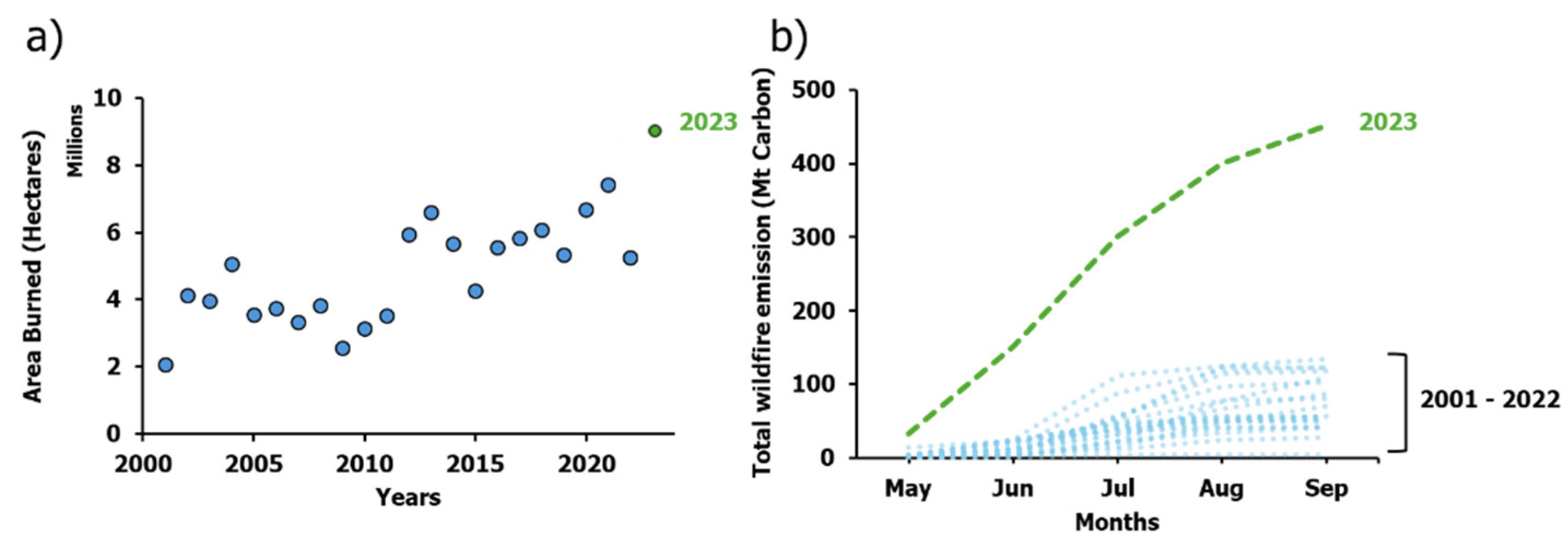
Figure 2.
Locations of ground-based Chl-a samples. Green and blue circles represent all the sampling lakes, while blue circles represent the lakes used for the Chl-a retrieval model development (matchups between in situ sampling and satellite overpass occurred within +/-3 days.
Figure 2.
Locations of ground-based Chl-a samples. Green and blue circles represent all the sampling lakes, while blue circles represent the lakes used for the Chl-a retrieval model development (matchups between in situ sampling and satellite overpass occurred within +/-3 days.
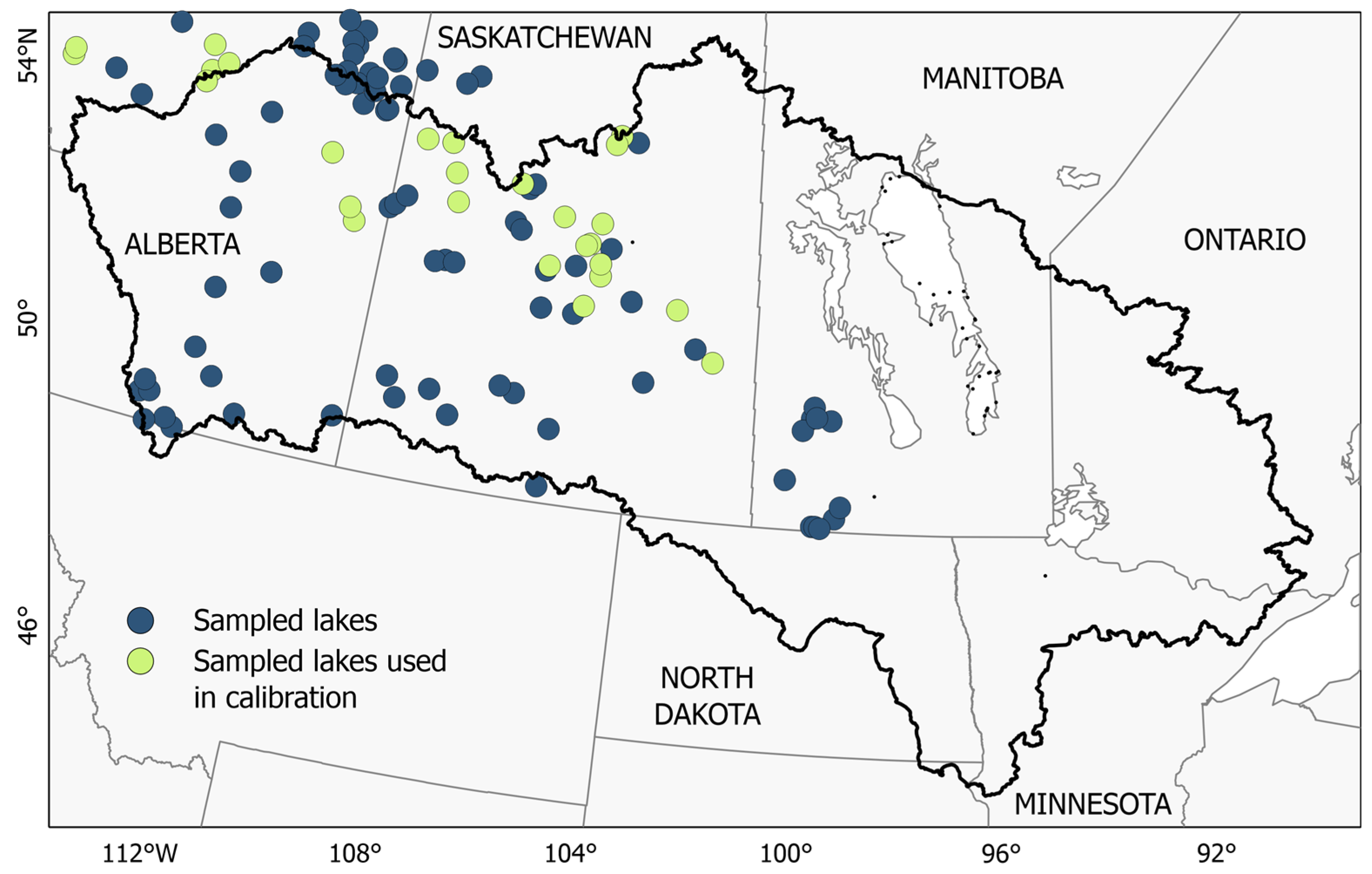
Figure 3.
The correlation between the band formulae and ln(Chl-a) for different temporal windows of in situ-satellite match-ups.
Figure 3.
The correlation between the band formulae and ln(Chl-a) for different temporal windows of in situ-satellite match-ups.
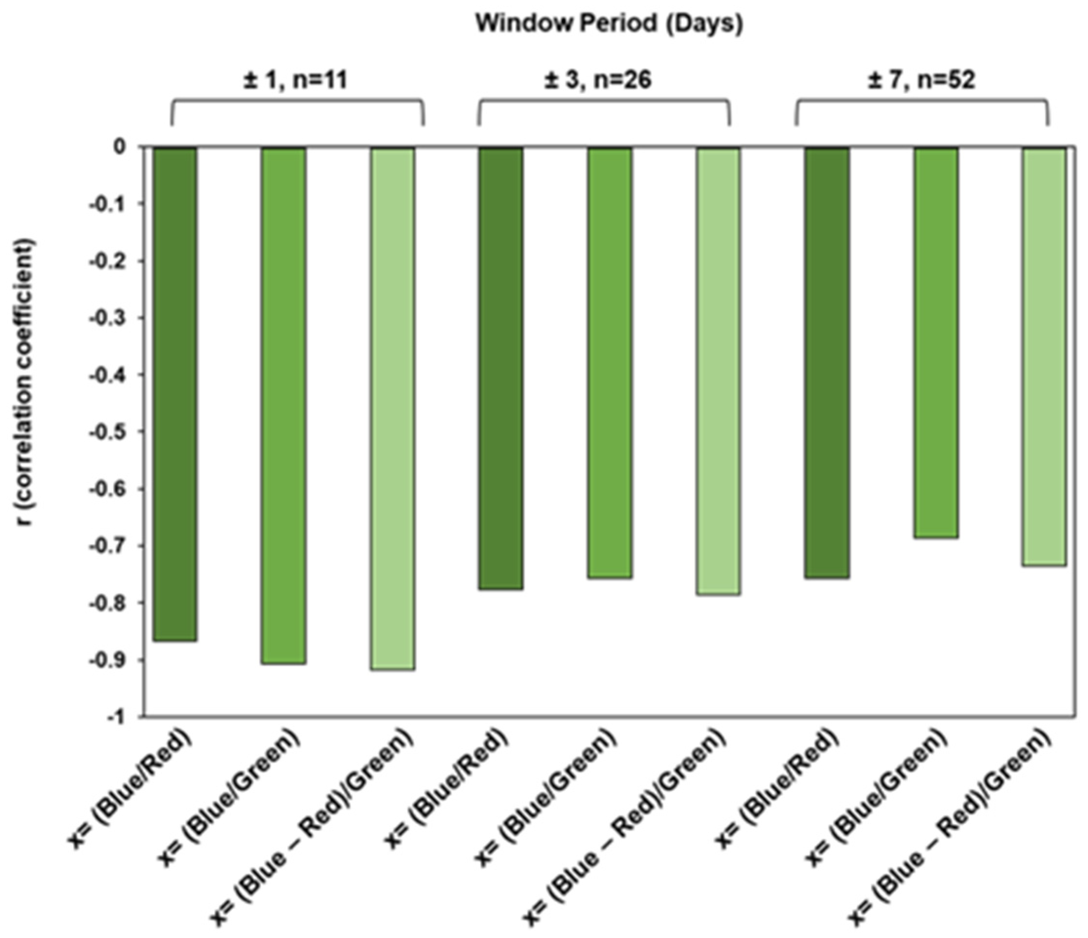
Figure 4.
Cluster analysis of B1 values with example images showing wildfire interference. “Wildfire Effect - 2023” showcases examples of lakes that were differentially affected by wildfire smoke, whereas “No Wildfire Effect - 2022” represents the same lakes in 2022, a year without wildfire interference.
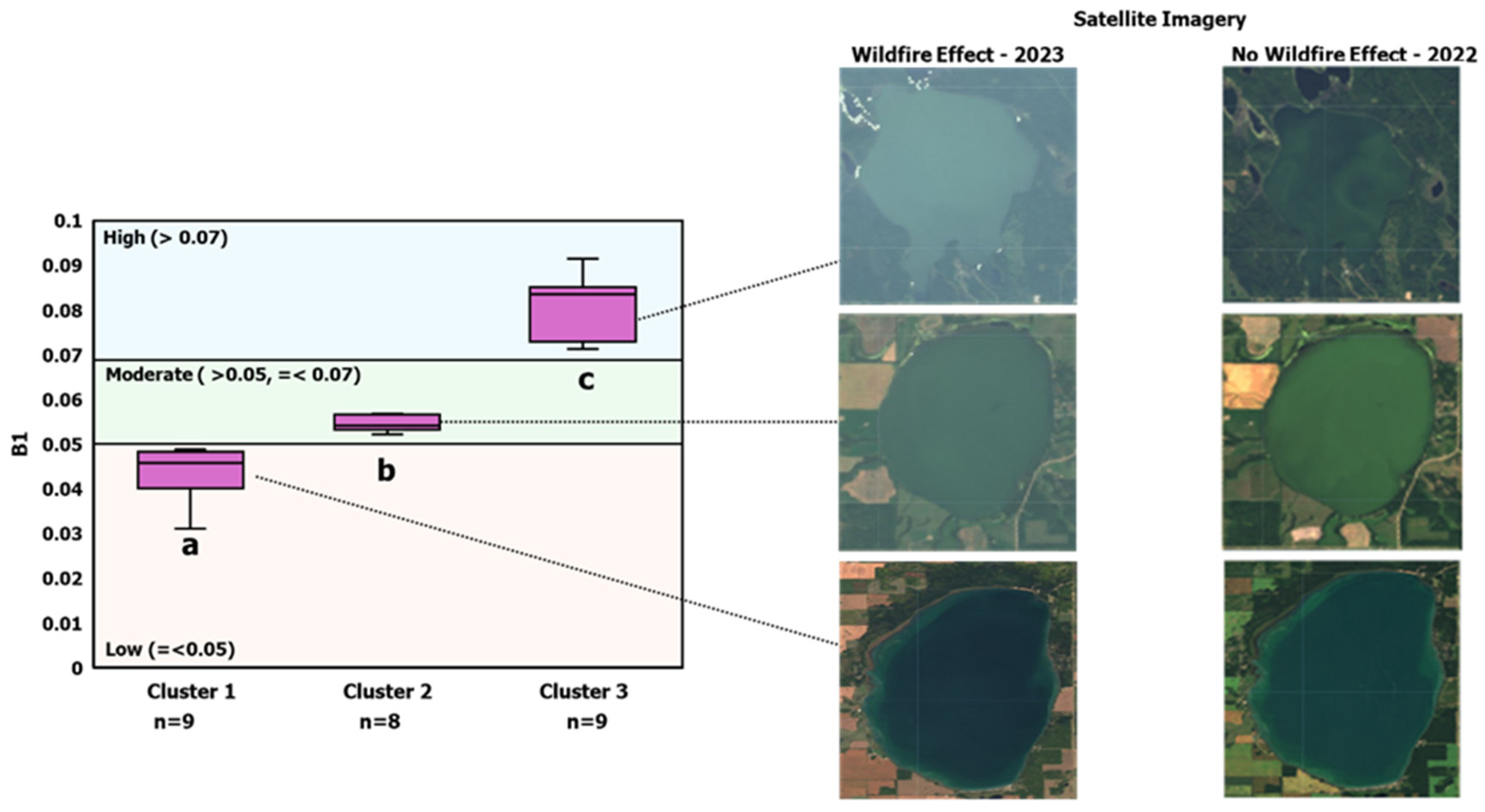
Figure 5.
The correlation between the band formulae and ln(Chl-a) for different temporal windows of in situ-satellite match-ups.
Figure 5.
The correlation between the band formulae and ln(Chl-a) for different temporal windows of in situ-satellite match-ups.
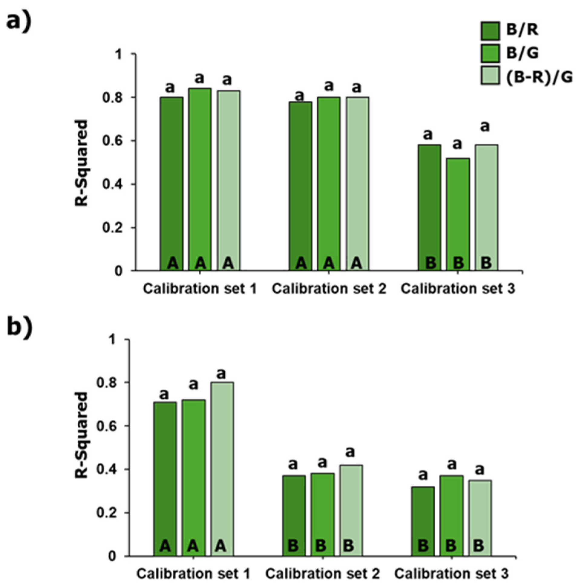
Figure 6.
a) Map of the differences in lake average Chl-a with and without B1 aerosol screening (with aerosol screening minus without) for the period from start of availability of Landsat OLI with B1 in 2013 to 2023. Frequency distributions of b) lake average Chl-a without aerosol screening, and c) with aerosol screening.
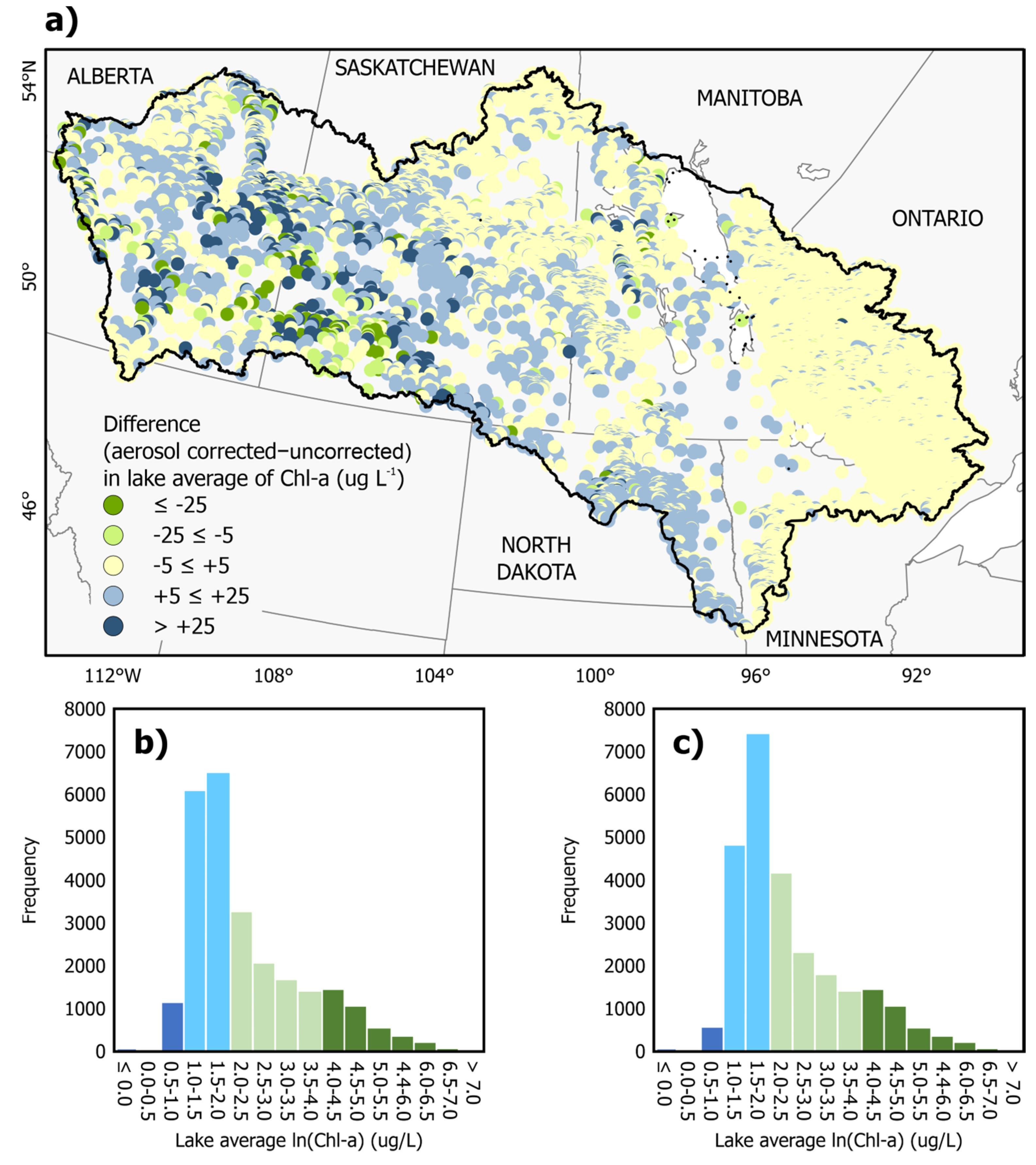

Table 1.
Summary of Landsat OLI bands and bandwidths used in this research.
| Sensor | Bands | Wavelengths (mm) | Resolution (m) |
|---|---|---|---|
| Landsat 8 OLI | Band 1: Coastal/Aerosol | 0.43-0.45 | 30 |
| Band 2: Blue | 0.45-0.51 | 30 | |
| Band 3: Green | 0.53-0.59 | 30 | |
| Band 4: Red | 0.64-0.67 | 30 | |
| Band 5: Near Infrared (NIR) | 0.85-0.88 | 30 | |
| Band 6: Shortwave Infrared (SWIR) | 1.57-1.65 | 30 |
Table 2.
Table of formulae used to calculate Rayleigh-corrected bottom-of-atmosphere (BOA) reflectance (Rrc) (Equations (1)–(7)) and to calculate model performance metrics (Equations (8)–(12)).
Table 2.
Table of formulae used to calculate Rayleigh-corrected bottom-of-atmosphere (BOA) reflectance (Rrc) (Equations (1)–(7)) and to calculate model performance metrics (Equations (8)–(12)).
| (1) | |
| where, is the TOA radiance for band , is the raw digital number (DN) for band , is the multiplicative rescaling factor for band and is the additive rescaling factor for band . |
|
| (2) | |
| where, is the Rayleigh path radiance, is the exo-atmospheric solar irradiance constant for band , is the solar zenith angle in degrees, is the satellite view angle in dgrees, is the Rayleigh phase function (Equation (3)), is the Rayleigh optical thickness for band (Equation (4)), and is the ozone transmittance for band (Equation (5)). |
|
| (3) | |
| where, is obtained from in which is the depolarization factor, and is the scattering angle in degrees (180 - ). |
|
| (4) | |
| (5) | |
| where, is the ozone optical thickness for band . |
|
| (6) | |
| where, is the Rayleigh-corrected radiance for band . |
|
| (7) | |
| where, is the partially corrected BOA reflectance for band , and d is the Earth–Sun distance in astronomical units. |
|
| (8) | |
| where, is the coefficient of determination, is the residual sum of square, and is the total sum of square. |
|
| (9) | |
| where, is Root Mean Square Error, is the predicted value, is the observed value, and n is the number of samples. |
|
| (10) | |
| where, is Normalized Root Mean Square Error, is the standard deviation of the observed values. |
|
| (11) | |
| where, is Mean Absolute Error |
|
| (12) |
Table 3.
The linear regression models developed for the three predictors using a +/- 3 days window based on a) partial atmospheric correction using Rayleigh-corrected reflectance and b) full atmospheric correction using the Landsat 8 level 2 process ready reflectance.
Table 3.
The linear regression models developed for the three predictors using a +/- 3 days window based on a) partial atmospheric correction using Rayleigh-corrected reflectance and b) full atmospheric correction using the Landsat 8 level 2 process ready reflectance.
| A. Partial atmospheric correction (Rayleigh-corrected reflectance) | |||||||||||||
|
Calibration set (Sample Size) |
Predictor | Correlation (r) | Chl-a Models | Train | Test | ||||||||
| R2 | RMSE | NRMSE | Bias | MAE | R2 | RMSE | NRMSE | Bias | MAE | ||||
|
1 (n = 9) |
x = (B/R) | -0.90 | ln(Chl-a) = -2.796*x+7.685 | 0.80 | 0.48 | 0.41 | 0 | 0.41 | 0.79 | 0.53 | 0.37 | 0.07 | 0.45 |
| x = (B/G) | -0.93 | ln(Chl-a) = -6.36*x+9.923 | 0.84 | 0.51 | 0.37 | 0 | 0.48 | 0.87 | 0.18 | 0.3 | -0.03 | 0.17 | |
| x = (B-R)/G | -0.95 | ln(Chl-a) = -5.988*x+5.61 | 0.83 | 0.43 | 0.37 | 0 | 0.38 | 0.99 | 0.10 | 0.08 | 0.05 | 0.08 | |
|
2 (n = 17) |
x = (B/R) | -0.89 | ln(Chl-a) = -2.646*x+7.342 | 0.78 | 0.52 | 0.45 | 0 | 0.40 | 0.74 | 0.64 | 0.46 | -0.09 | 0.58 |
| x = (B/G) | -0.90 | ln(Chl-a) = -4.631*x+8.017 | 0.80 | 0.45 | 0.42 | 0 | 0.38 | 0.77 | 0.68 | 0.43 | -0.01 | 0.55 | |
| x = (B-R)/G | -0.90 | ln(Chl-a) = -4.58*x+4.879 | 0.80 | 0.55 | 0.43 | 0 | 0.45 | 0.87 | 0.42 | 0.32 | 0.04 | 0.34 | |
|
3 (n = 26) |
x = (B/R) | -0.77 | ln(Chl-a) = -3.315*x+8.383 | 0.58 | 0.88 | 0.63 | 0 | 0.73 | 0.61 | 0.62 | 0.59 | 0.05 | 0.46 |
| x = (B/G) | -0.75 | ln(Chl-a) = -4.749*x+8.377 | 0.52 | 0.90 | 0.67 | 0 | 0.64 | 0.61 | 0.70 | 0.59 | 0.02 | 0.64 | |
| x = (B-R)/G | -0.78 | ln(Chl-a) = -4.685*x+5.016 | 0.58 | 0.85 | 0.63 | 0 | 0.60 | 0.68 | 0.63 | 0.53 | 0.06 | 0.58 | |
| B. Full atmospheric correction (Landsat 8 Level 2 reflectance) | |||||||||||||
|
Calibration set (Sample Size) |
Predictor | Correlation (r) | Chl-a Models | Train | Test | ||||||||
| R2 | RMSE | NRMSE | Bias | MAE | R2 | RMSE | NRMSE | Bias | MAE | ||||
|
1 (n = 9) |
x = (B/R) | -0.84 | ln(Chl-a) = -2.033*x+4.637 | 0.71 | 0.65 | 0.49 | 0 | 0.61 | 0.71 | 0.54 | 0.44 | 0.01 | 0.51 |
| x = (B/G) | -0.86 | ln(Chl-a) = -3.75*x+4.695 | 0.72 | 0.64 | 0.48 | 0 | 0.54 | 0.79 | 0.45 | 0.37 | -0.05 | 0.39 | |
| x = (B-R)/G | -0.88 | ln(Chl-a) = -4.331*x+2.501 | 0.8 | 0.47 | 0.41 | 0 | 0.41 | 0.74 | 0.65 | 0.41 | 0.00 | 0.60 | |
|
2 (n = 17) |
x = (B/R) | -0.67 | ln(Chl-a) = -2.157*x+5.121 | 0.37 | 0.95 | 0.76 | 0 | 0.76 | 0.64 | 0.74 | 0.53 | 0.00 | 0.56 |
| x = (B/G) | -0.66 | ln(Chl-a) = -2.981*x+4.787 | 0.38 | 0.87 | 0.75 | 0 | 0.74 | 0.46 | 1.03 | 0.66 | -0.10 | 0.85 | |
| x = (B-R)/G | -0.69 | ln(Chl-a) = -3.515*x+2.932 | 0.42 | 0.93 | 0.73 | 0 | 0.75 | 0.63 | 0.69 | 0.54 | -0.06 | 0.56 | |
|
3 (n = 26) |
x = (B/R) | -0.63 | ln(Chl-a) = -1.923*x+5.064 | 0.32 | 1.08 | 0.8 | 0 | 0.80 | 0.53 | 0.78 | 0.65 | 0.09 | 0.68 |
| x = (B/G) | -0.63 | ln(Chl-a) = -4.003*x+5.325 | 0.37 | 1.13 | 0.77 | 0 | 0.90 | 0.53 | 0.57 | 0.65 | -0.06 | 0.50 | |
| x = (B-R)/G | -0.63 | ln(Chl-a) = -3.867*x+3.018 | 0.35 | 1.06 | 0.78 | 0 | 0.81 | 0.52 | 0.79 | 0.66 | 0.09 | 0.59 | |
Disclaimer/Publisher’s Note: The statements, opinions and data contained in all publications are solely those of the individual author(s) and contributor(s) and not of MDPI and/or the editor(s). MDPI and/or the editor(s) disclaim responsibility for any injury to people or property resulting from any ideas, methods, instructions or products referred to in the content. |
© 2024 by the authors. Licensee MDPI, Basel, Switzerland. This article is an open access article distributed under the terms and conditions of the Creative Commons Attribution (CC BY) license (http://creativecommons.org/licenses/by/4.0/).
Copyright: This open access article is published under a Creative Commons CC BY 4.0 license, which permit the free download, distribution, and reuse, provided that the author and preprint are cited in any reuse.


