
Submitted:
08 August 2024
Posted:
12 August 2024
You are already at the latest version
Abstract
Building energy modelling tools play a crucial role in quantifying and comprehending the energy performance of buildings. These tools demand substantial amounts of data, which can be challenging to acquire and are often associated with significant uncertainties. The incorporation of Sensitivity Analysis represents a relevant step towards developing reliable models, as it identifies the most critical parameters that require a meticulous characterization. In this study, a Sensitivity Analysis based on Morris method was conducted to assess the relevance of 14 input parameters affecting thermal loads across four dwelling typologies modelled in EnergyPlus. Different number of Morris trajectories and levels were considered to analyse the impact of the user-defined values of r and p when employing Morris method. Convergence was achieved from r=200 and p=12, which are higher than the typically employed values (r=10 and p=4). Setpoint temperatures, orientation, roof solar absorptivity and roof conductance rank among the most relevant parameters affecting thermal loads, however variations are observed for the four case studies.
Keywords:
building energy model
; sensitivity analysis
; building simulation
Given the significant contribution of buildings to worldwide energy consumption, there is an increasing interest in quantifying and understanding their energy performance. Within this context, the use of Building Energy Model (BEM) tools has became increasingly popular in the evaluation and assessment of building energy performance [1,2,3,4]. These tools are usually data-intensive and the information needed to develop reliable models is difficult to obtain and subject to significant uncertainties [5,6]. This lack of information often leads to large mismatches between measured and simulated output data [7]. Therefore, for BEM tools to be employed with confidence, it is necessary for the models to be calibrated to represent the actual behaviour of the building under study [8].
As pointed out by Reddy et al. [9], standardized methods for calibrating BEMs involve defining a set of influential parameters. In this regard, the use of Sensitivity Analysis (SA) techniques can be useful for improving the understanding of the relationship between model inputs and outputs and for determining the most relevant parameters affecting building thermal performance [3,10]. Thus, SA of BEM input parameters represents an important step in the model calibration process and therefore increases confidence in the model results [6].
The methods for SA applied in BEM can be divided into local and global approaches. Sensitivity measures in Local Sensitivity Analysis (LSA) are calculated by changing one parameter while keeping the others constant at their reference value [4]. The main advantage of this method is that it is easily applied, and its results are easily interpreted. However, it only explores a reduced space of the input factor around a base case, and interactions between factors cannot be considered [11]. On the other hand, Global Sensitivity Analysis (GSA) focuses on the influence of uncertain inputs over the entire input space and is thus able to include effects from correlated input parameters. This category covers a range of methods applying different techniques, which usually evaluate the effect of an input parameter on the output by varying not only the parameter in question but also the other parameters chosen for the analysis [12]. This approach makes GSA methods more reliable but more computationally demanding than LSA.
Firth et al. [13] conducted a LSA for BEMs of six dwelling archetypes in the United Kingdom, aiming to assess the impact of input uncertainty on the predicted emissions of a housing stock model. Their analysis revealed that heating setpoint, length of the daily heating period, external air temperature, storey height, and gas boiler efficiency were the most influential parameters affecting emissions across most of the six archetypes. Similarly, Kavgic et al. [14] performed a LSA for dwelling archetypes in Serbia, identifying indoor temperature, heating system efficiency, and external air temperature as key parameters influencing space heating demand and, consequently, emissions. In another study, Lam et al. [15] conducted a LSA to examine the impact of 10 parameters on electricity use of 10 air-conditioned office buildings in Hong Kong. They found cooling setpoint, equipment loads and lighting loads to be the most relevant parameters affecting electricity use.
Demir Dilsiz et al. [16] carried out a GSA to analyze annual cooling and heating consumption for various building forms across different climates in the United States. Their findings highlighted that setpoint temperatures, infiltration rate, and the transmittance of walls, floors, and roofs were the input parameters with the most significant impact. In another study, Zhu et al. [17] conducted a GSA as part of a BEM calibration process for a three-storey office building in Colorado, United States. In this analysis, they determined that cooling setpoint, equipment and lighting power densities played key roles in cooling demand, while heating setpoint, occupancy density, and the solar heat gain coefficient of windows were critical factors affecting heating demand. Wang et al. [18] performed a GSA on a fictitious building in the Netherlands as a first step towards the calibration of an urban-scale energy model. The authors examined the influence of 14 parameters on heating demand and concluded that setpoint temperature, walls transmittance and infiltration rate were the parameters with highest impact.
The screening-based method is a specific group of the GSA methods in which the primary objective is often to fix some input factors from a large number of factors without reducing the output variance [11]. GSA methods of this type are considered useful for qualitatively identifying key design variables to which the model output is most sensitive, providing a computationally efficient alternative when a rough ranking of the parameters is desired [12]. The drawback of these methods is that they cannot quantify the effects of different factors on outputs, thus preventing the identification of how much of the total variances of outputs have been considered in the analysis [11]. The screening method described by Morris [19] is one of the most widely used methods for SA in BEM [3,4,6,12,20,21]. It can handle a large number of parameters while simultaneously requiring fewer simulations compared to other methods and providing easily interpretable results [10,11,20]. However, it is important to acknowledge that users of the Morris method often overlook the minimum number of simulations required to ensure result convergence.
Morris method is also widely used for SA in applications other than BEM. King and Perera [22] applied it to detect important variables on an urban water supply system, while Janse van Rensburg et al. [23] used it to approach the complexity of developing a physics-based model of a battery. Reuge et al. [24] used the method to identify the most sensitive parameters affecting a physicochemical model of chloride-induced corrosion of concrete in marine environments. Ben Touhami et al. [25] applied Morris method to examine the sensitivity of a pasture simulation model, while Han et al. [26] used it to identify key inputs in a biochemically-based photosynthesis model. Ujjwal et al. [27] analysed the uncertainty in a fire spread model, Aumond et al. [28] examined relevant parameters affecting a traffic noise model and Wang et al. [21] identified key parameters for a passive residual heat removal system.
In this study, the Morris method is applied to determine the most relevant parameters affecting cooling, heating and total thermal loads in four residential building typologies modelled in EnergyPlus. In Section 1, an overview of the Morris method is provided, along with a brief review of some previous studies that applied it to BEM. Additionally, there is a description of the Morris method parameters used in the present study. In Section 2, there is a description of the four case studies and the hypotheses considered in their EnergyPlus models. In Section 3 the convergence of the SA results with the user-defined parameters of the Morris method is analysed and the results are presented and discussed, and in Section 4 there are the conclusions of the study.
The novelty of this research lies in its pioneering approach toward developing high-fidelity BEMs tailored to the Uruguayan housing stock. The case studies are modeled with a level of detail not typically seen in comparable research, aiming to make them more representative of reality. They encompass multiple thermal zones, incorporate occupancy schedules dictating HVAC operation, account for occupants making use of solar protections and natural ventilation based on interior and exterior conditions and employ a comprehensive model (i.e., the EnergyPlus airflow network model) to simulate ventilation and infiltration loads, including airflow from both the exterior and adjacent zones.
Regarding the sensitivity analysis, special consideration has been given to the impact of user-defined parameters in the Morris method, which is not common practice when employing this method. Among the parameters under study, factors such as the solar absorptance of surfaces, often overlooked in similar studies, have proven to be highly relevant.
1. Methodology
A SA is conducted to identify relevant parameters in residential BEMs in Uruguay. The study involves four different building archetypes: three of them are typical buildings defined by Curto-Risso et al. [29] and the fourth is a social interest archetype modelled by Pena et al. [30]. For the analysis, the GSA technique introduced by Morris [19] is implemented.
1.1. Morris Method for Sensitivity Analysis
In the Morris method, the user must define the number of parameters under study (k) and their range of possible values. This determines , a k-dimensional input space consisting of the model inputs . is discretized into a p-level grid where each for may assume values within the grid.
For a given value of X, the Elementary Effect (EE) of the ith input factor is defined as the magnitude of variation in the model output due to a variation in the ith parameter (as shown in Eq. 1). By randomly sampling different X from , the finite distribution of (denoted ) is obtained.
In Eq. 1, is any selected value in , is the model output and is a predetermined multiple of .
The method assumes to follow a Gaussian distribution and utilizes its mean () and standard deviation () as indicators of the importance of the ith input. assesses the overall influence of the factor on the output, while estimates higher-order effects such as non-linearity or interactions with other inputs. Therefore, the Morris method identifies the inputs that can be considered to have an effect:
- Negligible (low and low ).
- Linear and additive (high and low ).
- Non-linear or involved in interactions with other inputs (high ).
Proposed by Campolongo et al. [31], a revised version of the measure is introduced, denoted . This measure represents the mean of the distribution of the absolute values of the EEs. The utilization of adresses a potential issue that may arise when includes both positive and negative elements (when the model is non-monotonic). In such instances, when calculating some effects may cancel each other out, leading to a low value even for an important factor. When is employed in place of , Garcia Sanchez et al. [3] propose that the value of identifies the inputs that are:
- Almost linear ().
- Monotonic ().
- Almost monotonic ().
- Non-monotonic or with high interactions with other factors ()
To estimate the sensitivity measures (or ) and , r EEs from each are sampled. The Morris method suggests a sampling strategy that entails generating r trajectories, each composed of points within the input space . At each point, one EE is computed for one input factor, resulting in a total of sample points. This translates to simulating building models.
Each trajectory is constructed by randomly selecting a base value from the p-level grid . Subsequently, all trajectory points are generated by incrementing (or decrementing) one of its k components at a time by . This design results in a trajectory comprising sampling points , where consecutive points differ in only one component by , and where each component has been increased (or decreased) once. This procedure is repeated r times, each time with randomly selected starting points.
Therefore, when employing the Morris method for SA, the user is required to specify not only the parameters to be analysed and their ranges of possible values but also the number of levels (p), the number of trajectories (r) and the value of . Morris [19] suggests that p should be an even number and should be set as . This choice ensures an equal probability of sampling from each .
1.2. Previous Studies Using Morris Method in BEM
Neale et al. [4] implemented the Morris method to identify a subset of the most influential parameters affecting electricity consumption and heating load in five Irish building archetypes: a two-storey detached dwelling, a two-storey semi-detached dwelling, a single-storey detached dwelling, a mid-floor apartment and a top-floor apartment. They selected 24 parameters for the scope of the analysis, including building construction parameters (U values), building energy use, building equipment parameters, ventilation and occupancy. For the apartment archetypes some of these parameters were not examined (the floor and roof U-values for the mid-floor apartment, for example) resulting in 19 and 22 parameters to evaluate in the mid-floor and top-floor apartments, respectively. The study employed a triangular distribution to describe the parameter input space, except for the orientation, for which a uniform distribution was assigned. They used a value of , resulting in 200-250 models for each archetype to simulate in EnergyPlus. There is no information provided regarding the values used for p and .
Garcia Sanchez et al. [3] conducted a SA using the Morris method in a seven-storey residential building with 32 dwellings. They employed ESP-r energy calculation software to model the building. In their analysis, the authors examined the impact on the heating load of 24 parameters. These parameters encompassed building design aspects (such as building and windows sizes, orientation and insulation thickness), operational factors (including temperature set-points, occupancy levels and ventilation rates), and meteorological variables (external temperature, solar radiation, ground reflectivity and wind speed). To ensure the analysis was representative of apartment buildings at a national level, the authors defined rather board intervals for possible parameter values. In their study, they set , and .
MauÄec et al. [32] utilized Morris method in six different timber building models developed in EnergyPlus. A total of 15 parameters where subjected to the analysis to assess their impact on heating and cooling thermal loads. These parameters included building geometry, insulation characteristics, glazing ratio and distribution, shading control and set-point temperatures. Three locations were considered, each with different climatic conditions: moderate, warm and cold. They evaluated the EE in trajectories, resulting in 160 simulations for each model. This led to a total of 2,880 simulations when considering the six building models and the three climate zones. There is no information provided regarding the values used for p and .
De Wit and Augenbroe [20] employed the Morris method in a naturally ventilated office located in the Netherlands. They subjected 89 parameters to the SA to evaluate their relative importance in assessing the uncertainty of a thermal comfort indicator defined as the number of hours per year that more than 10% of the occupants are dissatisfied with the climatic conditions in the building. The authors assumed normal distributions for all parameters. They conducted simulations using two thermal building model tools: ESP-r and BFEP. For the SA, they assessed five independent samples of the EE on the comfort performance indicator () resulting in a total of 450 simulation runs. There is no information provided regarding the values used for p and .
Petersen et al. [12] conducted a study to examine the impact of the choice of p and r on the results obtained from the Morris method. They compared these results with those obtained using the Sobol method. The case of study was a one-storey office building modelled in EnergyPlus. The authors found that, in order for the Morris method to identify the same cluster of parameters as the Sobol method, it required a higher value of r than what is typically applied. The authors commented on the limited attention given to the effect of the user-defined values for p and r when applying Morris method in BEM. As a result of their study, they recommend using and conducting simulations in steps of to qualitatively analyse convergence.
Menberg et al. [6] utilized the Morris method in a case study employing TRNSYS as the simulation tool. Their study focused on the Architecture Studio at the University of Cambridge, using the annual heating demand of the first floor as the quantity of interest in the SA. The authors selected 11 uncertain parameters within the TRNSYS model and defined board ranges for their possible values. The aim was to assess the performance of the SA method in situations with limited information about the actual parameter values. All parameters were assumed to follow uniform distributions. The researchers explored the method using different numbers of trajectories to identify the minimum value of r required for a robust ranking of parameters. They performed 10 independent evaluations of the Morris method, each with 10 trajectories, and observed significant variations in both and across the 10 independent evaluations. Their conclusion was that the method performed reasonably well when .
1.3. Implementation
In this study, the Morris method is employed to assess the influence of 14 uncertain parameters () on the annual heating and cooling requirements of four dwelling typologies. The buildings are modelled and simulated using EnergyPlus, while Python functions are utilized for designing the Morris samples, generating and executing the models, and processing the SA results. Taking into consideration the assessment by Petersen et al. [12] regarding the importance of analysing the impact of the selected values for p and r, four different levels are explored (, 8, 12 and 16) in trajectories. This is a higher number of trajectories than what is typically chosen by Morris method users, and results in 6,000 simulations for each building typology and each value of p, leading to a grand total of 96,000 simulations.
Given that the aim of this analysis is to identify the input parameters crucial for describing the building stock as accurately as possible at a national level, broad ranges are defined for the parameters under study and uniform distributions are considered. The selected parameters and their variation ranges are presented in Table 1. The term conductance, denoted as , represents the inverse of the sum of conduction resistances. The air permeability of windows is characterized by the air mass flow coefficient when the opening is closed per unit length at 1 Pa (denoted ). Windows blinds activation criteria establishes the level of solar irradiation on windows above which blinds are activated when the cooling system is in operation.
The ranges for conductances, thermal capacitances and air permeability are determined based on the minimum and maximum values defined for the Uruguayan housing stock in Curto-Risso et al. [29]. For orientation and solar absorptivities, the ranges encompass all possible values, while for blinds activation criteria, a broad range is defined. In the case of heating and cooling setpoints, narrower ranges are considered to prevent distorting the problem; for example, ensuring that the cooling setpoint is not lower than the heating setpoint.
Regarding the window-to-wall (WWR) and occupancy, the ranges are set as wide as possible while remaining reasonable for each typology. This results in different ranges for the four different case studies. The criteria for determining the WWR range involve maximizing (or minimizing) the size of existing windows wherever possible, with the exception of bathroom windows. For occupancy, a minimum floor area of 8 m²/person was established.
The value used for is set as as recommended by Morris [19]. The only exception is the value of used to vary the orientation which is . The reason behind this exception is that for the orientation results in values of angle variation of around 180º and in most of the case studies (due to the windows and exposed walls location) there is a rather cyclical relationship between energy consumption and orientation, with a period of 180º. Therefore, using for the orientation could lead to a low value even when orientation has a significant impact on energy consumption. This approach aligns with what is suggested by Morris [19] of assigning different values of to some inputs when some prior knowledge of the function Y makes it desirable. Additionally, as orientation is a circular parameter (a step of from the maximum value, returns the orientation to 0º), equal probability sampling is ensured regardless of the value used for .
1.4. Limitations of the Research
The selected SA approach provides a qualitative identification of input factors to which thermal loads are more sensitive, but does not quantify the effects of the different parameters on the outputs.
This study is limited to the four studied typologies and focuses on identifying the most relevant parameters affecting thermal loads among the 14 proposed parameters. Climatic factors such as exterior temperatures, irradiation, wind speed and direction, and precipitation were not considered. Additionally, the configuration of the surroundings, such as neighboring buildings or vegetation, was not included in the analysis. The design and dimensioning of heating and cooling systems and their efficiency were also not considered. The behavior of occupants is only accounted for through temperature setpoints and window blind activation criteria.
2. Case Studies
The study employs three of the building archetypes developed by Curto-Risso et al. [29] and a social interest building modelled by Pena et al. [30] and Favre et al. [33]. These are:
- A 27 m single-storey detached dwelling, hereafter referred to as the "house-studio".
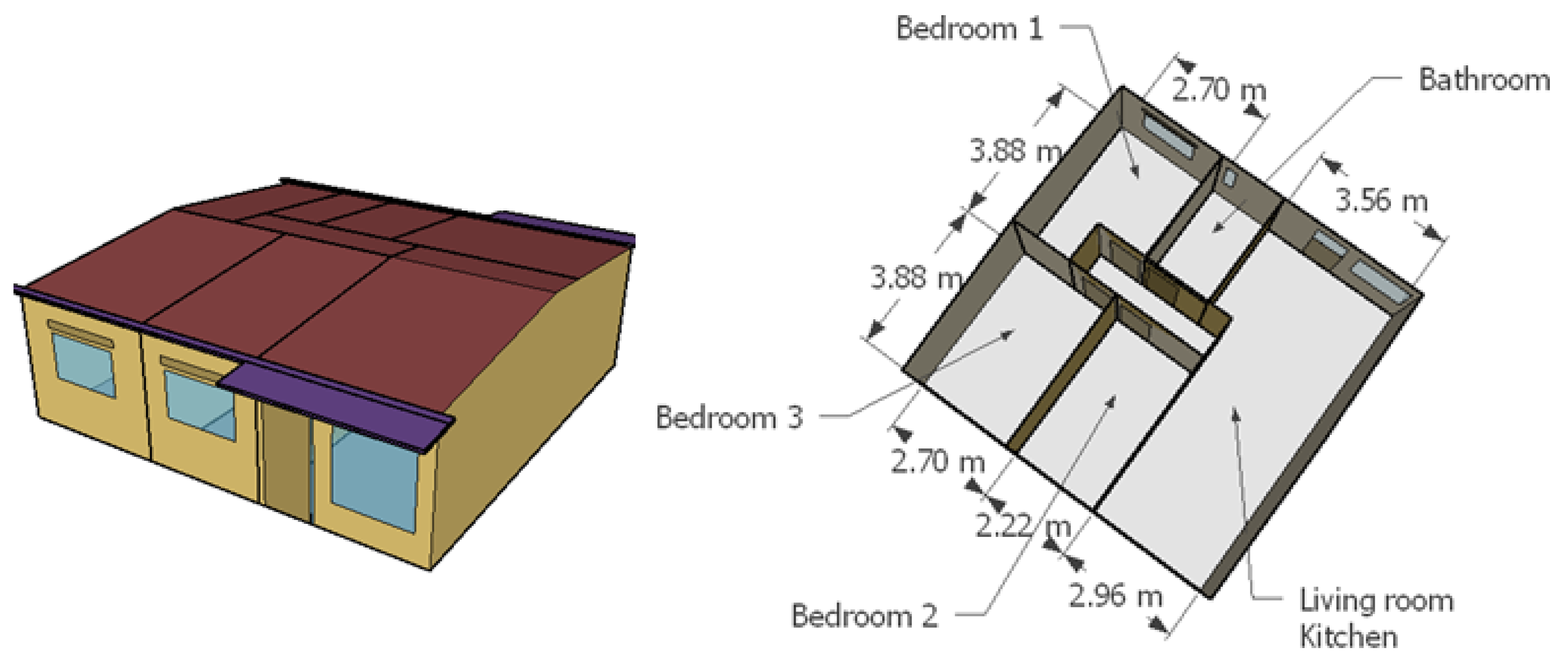
- A 53 m two-storey attached dwelling, hereafter referred to as the "two-storey".
- A 117 m single-storey detached dwelling, hereafter referred to as the "ranch".
- A 66 m single-storey detached dwelling, hereafter referred to as the "bungalow".
The case studies are illustrated in Figure 1 to Figure 4. EnergyPlus models of these four typologies are employed for the SA and the weather file used for the simulations is the Typical Meteorological Year (TMY) of Montevideo in Uruguay, a city with a temperate climate. In the models, the thermal zones of the dwellings remain consistent with their original definitions in Curto-Risso et al. [29], Pena et al. [30] and Favre et al. [33]. The inside and outside convection coefficients are calculated using the defaults TARP and DOE-2 models. Solar distribution is modelled as full exterior and a simulation timestep of 10 minutes is utilized. The HVAC systems are modelled with the ideal load air system and are only considered in the occupied zones. Ventilation and infiltration loads are solved using the airflow network model.
The occupancy criteria are as follows: the main living room (denoted living room 1 when there is more than one living room) is occupied by 50% of the dwelling occupants from 14 to 18 hs and by 100% from 18 to 22 hs. The bedrooms are occupied from 22 to 8 hs, with 2 occupants using the largest bedroom (denoted bedroom 1), and the remaining occupants are distributed among the other bedrooms. For example, in a case with 3 people and 2 bedrooms, 2 people occupy the largest bedroom and one person occupies the other. In a case with 3 people and 3 bedrooms, 2 people occupy the largest bedroom, one person occupies the second largest, and the third bedroom remains unoccupied. No occupation is considered for living rooms other than living room 1 and bathrooms. The occupancy schedules are crucial because the HVAC system is only available when the zone is occupied, thus an empty bedroom does not consume energy from the HVAC system, at least directly.
Figure 3.
Ranch.
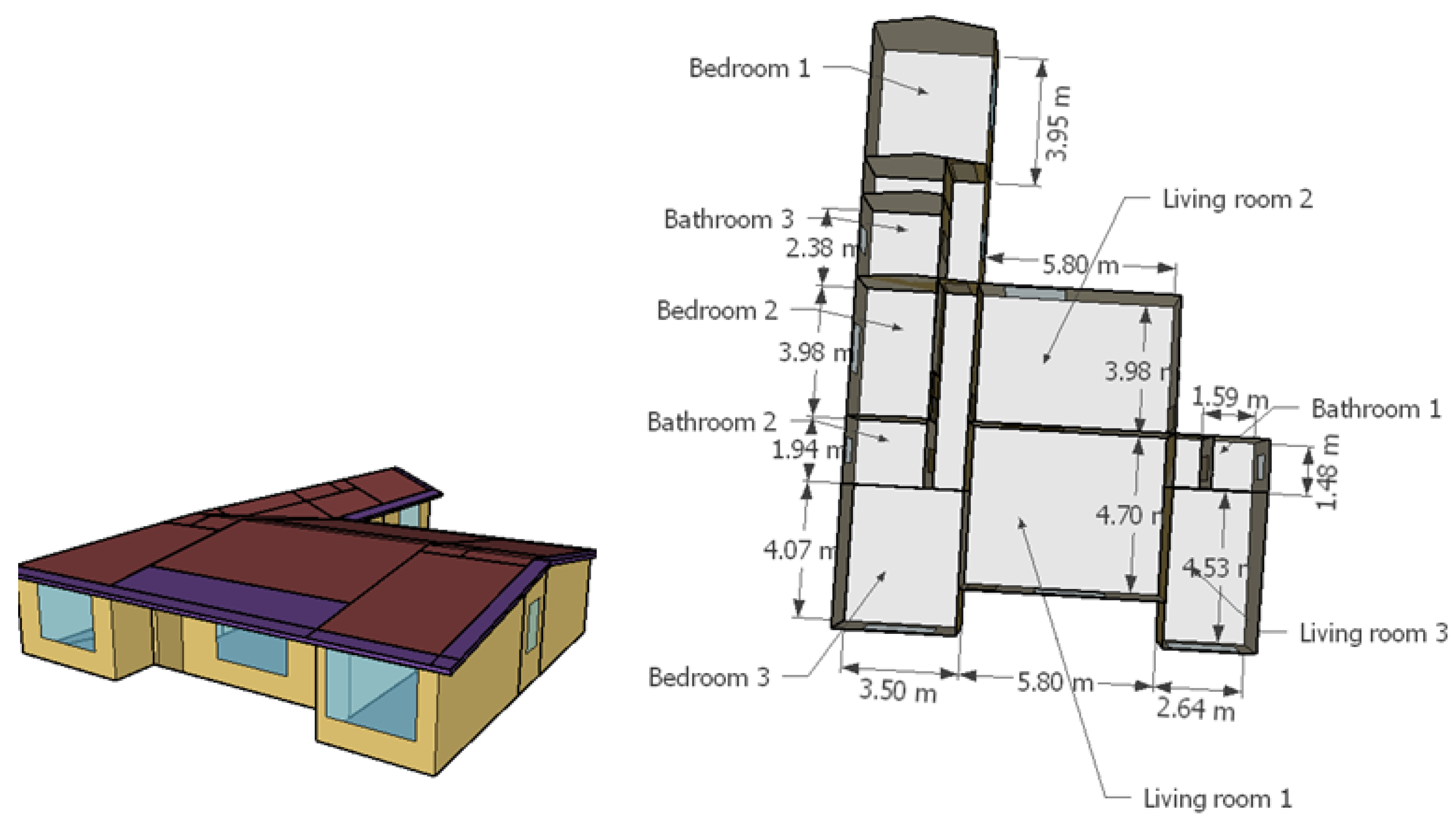
Figure 4.
Bungalow.
The construction materials for floors, interior walls, ceilings and doors remain consistent with their original definitions in Curto-Risso et al. [29] and Pena et al. [30]. However, for the exterior walls, roofs and windows, new fictional materials are defined. These materials are adjusted in terms of conductivity, density and solar absorptivity to meet the required conductances, thermal capacitances and solar absorptivities. Additionally, for the windows, the air mass flow coefficient when the opening is closed is adjusted according to the value of the air permeability parameter.
All exterior windows are equipped with blinds. In occupied zones, the blinds are activated when cooling is on and solar irradiation exceeds the specified threshold defined by the blinds activation criteria parameter. In unoccupied zones, the blinds are activated when zone temperature exceeds 23ºC and solar irradiation exceeds the specified threshold parameter.
3. Results and Discussion
Considering the assessment by Petersen et al. [12] regarding the importance of analysing the impact of the selected values for p and r in the SA results, four levels are evaluated (, 8, 12 and 16) in a total of trajectories. In this study, the classification of parameters by order of importance is based on the value of , as elaborated later. Thus, to analyse the number of trajectories required, the resulting for each parameter is assessed in steps of to visually analyse its convergence. On the other hand, the impact of p is studied qualitatively by observing the resulting ranking of the parameters for the different values of p considered.
For the four studied typologies, up to there are important variations in the results (see Figure 5 and Figure 6 with the results for cooling and heating requirements, respectively). From results seem to have converged. Ranking changes that occur for larger values of r are between parameters with very similar final values, which should therefore be considered as equally relevant.
Regarding the impact of the defined number of levels (p), the findings reveal that changes in the obtained ranking occur up to (see Figure 7 and Figure 8). However, the most substantial variations are observed up to . Changes between results for and primarily involve parameters with very similar values, indicating their roughly equal relevance.
For and the cooling, heating and total thermal loads in the four typologies fall within the ranges presented in Table 2. The considerable variability in the results for different combinations of the input parameters underscores the significant impact of the selected parameters on the thermal loads; at least for the wide ranges of variation considered.
The results from the Morris method are presented by plotting the and of the EE for the parameters under study for cooling, heating and total thermal loads. Low values of both and indicate a non-influential parameter and the greater the distance from (0,0) the more relevant the parameter (circles centered at (0,0) are plotted for reference). The , 0.5 and 1 are plotted to delimit the linear, monotonic, almost monotonic and non-monotonic or with high interactions with other factors zones.
The EE analysis for the house-studio (see Figure 9) shows that roof solar absorptivity, cooling setpoint, walls solar absorptivity, orientation and roof conductance are the parameters with the highest impact on cooling loads. The first three are all in the monotonic region () whereas the orientation and the roof conductance are either non-monotonic or involved in interactions with other factors (). For heating loads, the heating setpoint, roof solar absorptivity, roof conductance, walls solar absorptivity and walls conductance are the most influential parameters; all in the monotonic or almost-monotonic regions (). Finally, when considering total thermal loads (cooling + heating), roof solar absorptivity, cooling setpoint, roof conductance, heating setpoint and orientation are the most relevant parameters. The first four in the monotonic or almost-monotonic regions () while the orientation is either non-monotonic or involved in interactions with other factors ().
For the two-storey typology (see Figure 10), the orientation, cooling setpoint, occupancy, roof solar absorptivity and window-to-wall ratio have the highest impact on cooling loads; all in the monotonic region () except for the orientation which is either non-monotonic or involved in interactions with other factors (). Heating setpoint, orientation, roof conductance, roof solar absorptivity and occupancy are the key parameters affecting heating loads; the orientation and occupancy are non-monotonic or involved in interactions with other factors () whereas the other three are monotonic or almost monotonic (). For total thermal loads, the orientation, occupancy, cooling setpoint, roof solar absorptivity and heating setpoint are the most influential parameters; all in the monotonic or almost monotonic regions (), except for the orientation.
Results for the ranch typology (see Figure 11) show that roof solar absorptivity, cooling setpoint, occupancy and roof conductance are the key parameters for cooling loads; the first three are in the monotonic region whereas the roof conductance is non-monotonic or involved in interactions with other factors (). Heating setpoint, roof solar absorptivity, roof conductance and occupancy have the highest influence on heating loads, all in the monotonic or almost monotonic regions (). Considering total thermal loads, roof solar absorptivity, cooling setpoint, roof conductance, occupancy and heating setpoint are the most relevant parameters all in the monotonic or almost monotonic regions ().
Results for the bungalow EE analysis (see Figure 12) show that roof solar absorptivity, cooling setpoint, orientation, occupancy and roof conductance are the key parameters for cooling loads. The orientation and the roof conductance in the non monotonic or with relevant interactions region () and the others in the monotonic or almost monotonic regions (). Heating setpoint, roof solar absorptivity, occupancy and roof conductance have the most influence on heating loads all in the monotonic or almost monotonic regions (), except for the occupancy which is either non monotonic or involved in interactions with other parameters (). For total thermal loads, the key parameters are roof solar absorptivity, occupancy, orientation, cooling setpoint and roof conductance all in the monotonic or almost monotonic regions (), except for the orientation which is either non monotonic or involved in interactions with other parameters ().
Analysing the EE results for all four case studies, both for cooling and heating loads, roof solar absorptivity, setpoint temperatures, orientation and roof conductance are among the parameters with greatest impact independently of the typology. On the other hand, windows conductance, walls thermal capacity and windows air permeability have the lowest impact on cooling, heating and total thermal loads for all four case studies.
The occupancy has high impact on cooling, heating and total thermal loads for all typologies with exception of the house-studio. This is reasonable given that in the house-studio, the occupancy takes values in a narrower range than in the other typologies (see Table 1) and also that there is only one area for thermal conditioning; while in the other three typologies conditioned area changes with changes in the amount of occupants (depending on the number of occupied bedrooms), in the house-studio it does not.
The orientation parameter appears to have a more significant impact on the two-storey and bungalow typologies. This can be attributed to the fact that these typologies only feature windows on the front and rear facades, whereas the other typologies have windows facing all four directions. Additionally, the two-storey model is attached on both sides, further emphasizing the relevance of orientation.
Walls and roof conductances are more relevant for heating than for cooling loads; whereas the opposite is true for WWR and blinds activation criteria. Conductances being more relevant for heating loads might be because temperature difference between inside and outside is grater in winter than in summer, making heat transferred through walls and roof higher for a given U-value. WWR has higher impact on cooling loads given that there are more energy gains through windows in summer than in winter, especially in east, south and west facing windows which have rather small (zero for south) solar gains during winter. It is also reasonable for blinds activaction criteria to be more relevant for cooling loads as the blinds are activated if cooling is on or if there is high temperature in an unoccupied zone.
As a syntethis, the Morris resulting top 5 most influential parameters for cooling and heating loads across the four typologies are presented in Table 3. Roof solar absorptivity, setpoint temperatures, orientation and roof conductance consistently rank among the most influential parameters in all the four studied typologies. Occupancy in also in the top 5 most relevant parameters for all typologies, except for the house-studio.
Neale et al. [4], for an Irish residential typology similar to the bungalow of this study, also found that heating setpoint, occupancy and roof transmittance are among the most relevant parameters affecting heating loads. However, and contrarily to the results obtained in this study, the authors found windows transmittance to be quite relevant and not the roof solar absorptivity. These differences might be due to the different climatic characteristics, as in Irish winter there is less solar irradiation and lower exterior temperatures than in Uruguayan winter.
Petersen et al. [12], for a Danish one-storey attached office, found that orientation is one of the most influential parameters both in heating and cooling loads. These findings align with the results obtained in this study, where orientation emerged as the most significant factor in the attached typology. Heating and cooling setpoints were also identified as relevant parameters, and roof insulation is among the key parameters for heating loads, also coherent with the results obtained in this study for roof conductance. The authors did not include solar absorptivities in their analysis.
Neale et al. [4] and Petersen et al. [12] found ventilation rates, equipment loads and solar heat gains coefficient of the windows to be relevant parameters, which were not subject of this study. Ventilation rates were not considered as input parameters because in Uruguayan dwellings, ventilation is typically managed by occupants through window operation rather than central systems. Therefore, characterizing ventilation rates for a specific typology is not reasonable, as they depend on occupant behaviour. On the other hand, equipment loads were not included in this study, as it was assumed that there is not much variation of this parameter among Uruguayan dwellings. This assumption differs from Neale et al. [4], who considered a wide range of equipment loads in a single-family dwelling. Lastly, this study did not examine the solar heat gain coefficient of windows, as the use of treated window panes to manage solar gains is not widespread in Uruguayan dwellings.
In the study by Garcia Sanchez et al. [3], which focused on a residential apartment building, the authors concluded that temperature setpoint and number of occupants are some of the key parameters affecting heating loads. This aligns with the findings of this study and of the reviewed studies in general. Additionally, Garcia Sanchez et al. [3] identified insulation thickness in walls as one of the most relevant inputs. This is a reasonable outcome for a seven-storey building, where the role of walls in terms of heat transfer becomes more critical compared to the roof.
Menberg et al. [6] similarly identified temperature setpoint as the key parameter affecting heating loads. However, they also found that infiltration rate is among the most relevant factors, which differs from the results obtained in this study, where air permeability of windows did not have a significant impact.
In the study by De Wit and Augenbroe [20], the focus was on environmental factors, which were not considered in this study. Therefore, their findings might not directly align with the results presented here.
4. Conclusions
The Morris method was applied in this study to conduct SA on four typologies representative of the Uruguayan housing stock, modeled using EnergyPlus. The main goal was to determine which parameters require detailed characterization for the development of accurate energy models. The study examined 14 parameters, with a majority related to building construction properties (walls and roof conductances, solar absorptivities and thermal capacitances, WWR, orientation and window permeability). Additionally, parameters related to building operation, such as setpoint temperatures, number of occupants and window blinds operation criteria, were considered. Uniform distributions with wide ranges were used for all these parameters.
The SA contemplated the use of four different levels (, 8, 12 and 16) and a higher number of trajectories than typically used in Morris method SA (). This was done to assess the influence of the user-defined values of p and r. The results indicate that for , convergence was achieved after 200 trajectories and for practically the same rankings were obtained for and , but not for the lower values of p.
It is important to note that for , a number of trajectories frequently employed in SA using the Morris method, convergence of results was not achieved in this study. This observation raises a significant concern regarding the computational cost of the Morris method. While this method is often commended for its computational efficiency, the findings of this study suggest that achieving convergence and reliable results may require a substantially higher number of trajectories, such as . Nevertheless, it is noteworthy that the number of simulations typically required for the Morris method with remains significantly lower than the number of simulations typically required by other methods. For instance, studies employing the Sobol method for SA in BEM have demanded between 10,000 and 250,000 simulations per model [4,6,12,34].
The results of the EE analysis reveal that certain parameters consistently rank among the most relevant in all four studied typologies, aligning with findings in previous research. Conversely, some parameters identified as significant in this study were not important or were not even examined in the reviewed studies, and vice versa.
This study identified setpoint temperatures, roof solar absorptivity, roof conductance and orientation among the most relevant parameters across all four case studies. Occupancy emerged as a critical parameter for all typologies except the house-studio, where the maximum number of occupants is low, and the conditioned area remains constant regardless of the number of occupants. Additionally, in the context of heating loads, walls solar absorptivity was found to be a significant input, along with walls conductance.
Differences in the results obtained with other studies might be explained, in some cases, by different climatic conditions and/or building characteristics. In other cases, there are important differences in the set of parameters selected for the analysis and their ranges of possible variations. These definitions depend on the objective of the analysis as well as on the expertise and knowledge of the local reality of the person doing it. This shows that the SA results are difficult to extrapolate to different countries thus proving the importance of performing local studies.
In summary, the main results of this study are as follows:
- Achieving convergence and reliable results using the Morris method for SA may require a higher number of trajectories and levels than typically employed, such as r = 200 and p=12. Yet, the number of simulations required is still lower than those required by other methods (e.g., Sobol method).
- Key parameters identified across all case studies include: setpoint temperatures, roof solar absorptivity, roof conductance and orientation.
- Occupancy was a critical parameter for all typologies except the house-studio.
- Solar absorptivity and conductance of walls were significant for heating loads.
- SA results are difficult to extrapolate to different countries due to different climatic conditions, different characteristics of buildings and thermal conditioning systems and cultural aspects related to housing use. This highlights the importance of local studies.
Data Availability Statement
The input files for the study are available here. Further details are available from the corresponding author, Sofà a Gervaz, upon reasonable request.
List of abbreviations
| BEM | Building Energy Model |
| EE | Elementary Effect |
| GSA | Global Sensitivity Analysis |
| HVAC | Heating Ventilation & Air Conditioning |
| LSA | Local Sensitivity Analysis |
| SA | Sensitivity Analysis |
| TMY | Typical Meteorological Year |
List of symbols
| C | Thermal capacitance |
| Air mass flow coefficient when de opening is closed per unit length at 1Pa | |
| CSP | Cooling setpoint temperature |
| Morris method ith input elementary effect | |
| Finite distribution of EE_i | |
| HSP | Heating setpoint temperature |
| k | Number of parameters under study in Morris method |
| p | Morris method levels |
| r | Morris method trajectories |
| U | Transmittance |
| Conductance; the inverse of the sum of conduction resistances | |
| WWR | Wintow-to-wall ratio |
| Morris method ith input | |
| Y | Morris method output |
| Solar absorptivity | |
| Morris method increment | |
| Mean | |
| Absolute mean | |
| Morris method k-dimensional input space | |
| Standard deviation |
References
- Corrado, V.; Mechri, H.E. Uncertainty and sensitivity analysis for building energy rating. Journal of Building Physics 2009, 33, 125–156.
- Fabrizio, E.; Monetti, V. Methodologies and advancements in the calibration of building energy models. Energies 2015, 8, 2548–2574.
- Garcia Sanchez, D.; Lacarrière, B.; Musy, M.; Bourges, B. Application of sensitivity analysis in building energy simulations: Combining first- and second-order elementary effects methods. Energy and Buildings 2014, 68, 741–750.
- Neale, J.; Haris, M.; Mangina, E.; Finn, D.; O’ Donnell, J. Accurate identification of influential building parameters through an integration of global sensitivity and feature selection techniques. Applied Energy 2022, 315, 118956.
- Heo, Y.; Choudhary, R.; Augenbroe, G.A. Calibration of building energy models for retrofit analysis under uncertainty. Energy and Buildings 2012, 47, 550–560.
- Menberg, K.; Heo, Y.; Choudhary, R. Analysis of uncertainty in building design evaluations and its implications. Energy and Buildings 2002, 34, 951–958.
- Li, S.; Deng, K.; Zhou, M. Sensitivity Analysis for Building Energy Simulation Model Calibration via Algorithmic Differentiation. IEEE Transactions on Automation Science and Engineering 2017, 14, 905–914.
- Coakley, D.; Raftery, P.; Keane, M. A review of methods to match building energy simulation models to measured data. Renewable and Sustainable Energy Reviews 2014, 37, 123–141.
- Reddy, T.; Maor, I.; Panjapornpon, C. Calibrating Detailed Building Energy Simulation Programs with Measured Data - Part I: General Methodology (RP-1051). HVAC and R Research 2007, 13, 221–241.
- Heiselberg, P.; Brohus, H.; Hesselholt, A.; Rasmussen, H.; Seinre, E.; Thomas, S. Application of sensitivity analysis in design of sustainable buildings. Renewable Energy 2009, 34, 2030–2036.
- Wei, T. A review of sensitivity analysis methods in building energy analysis. Renewable and Sustainable Energy Reviews 2013, 20, 411–419.
- Petersen, S.; Kristensen, M.H.; Knudsen, M.D. Prerequisites for reliable sensitivity analysis of a high fidelity building energy model. Energy and Buildings 2018, 183, 1–16.
- Firth, S.K.; Lomas, K.J.; Wright, A.J. Targeting household energy-efficiency measures using sensitivity analysis. Building Research and Information 2010, 38, 25–41.
- Kavgic, M.; Mumovic, D.; Summerfield, A.; Stevanovic, Z.; Ecim-Djuric, O. Uncertainty and modeling energy consumption: Sensitivity analysis for a city-scale domestic energy model. Energy and Buildings 2013, 60, 1–11.
- Lam, J.; Wan, K.; Yang, L. Sensitivity analysis and energy conservation measures implications. Energy Conversion and Management 2008, 49, 3170–3177.
- Demir Dilsiz, A.; Ng, K.; Kämpf, J.; Nagy, Z. Ranking parameters in urban energy models for various building forms and climates using sensitivity analysis. Building Simulation 2023, 16, 1587–1600.
- Zhu, C.; Tian, W.; Yin, B.; Li, Z.; Shi, J. Uncertainty calibration of building energy models by combining approximate Bayesian computation and machine learning algorithms. Applied Energy 2020, 268, 115025.
- Wang, C.; Peng, M.; Xia, G. Sensitivity analysis based on Morris method of passive system performance under ocean conditions. Annals of Nuclear Energy 2020, 137, 107067.
- Morris, M.D. Factorial sampling plans for preliminary computational experiments. Technometrics 1991, 33, 161–174.
- De Wit, S.; Augenbroe, G. Analysis of uncertainty in building design evaluations and its implications. Energy and Buildings 2002, 34, 951–958.
- Wang, C.K.; Tindemans, S.; Miller, C.; Agugiaro, G.; Stoter, J. Bayesian calibration at the urban scale: a case study on a large residential heating demand application in Amsterdam. Journal of Building Performance Simulation 2020, 13, 347–361.
- King, D.; Perera, B. Morris method of sensitivity analysis applied to assess the importance of input variables on urban water supply yield â A case study. Journal of Hydrology 2013, 477, 17–32.
- Janse van Rensburg, A.; van Schoor, G.; van Vuuren, P. Stepwise Global Sensitivity Analysis of a Physics-Based Battery Model using the Morris Method and Monte Carlo Experiments. Journal of Energy Storage 2019, 25, 100875.
- Reuge, N.; Bignonnet, F.; Bonnet, S. Sensitivity analysis of a physicochemical model of chloride ingress into real concrete structures subjected to long-term exposure to tidal cycles. Applied Ocean Research 2023, 138, 103622.
- Ben Touhami, H.; Lardy, R.; Barra, V.; Bellocchi, G. Screening parameters in the Pasture Simulation model using the Morris method. Ecological Modelling 2013, 266, 42–57.
- Han, T.; Feng, Q.; Yu, T. Parameter sensitivity analysis for a biochemically-based photosynthesis model. Research in Cold and Arid Regions 2023, 15, 73–84.
- Ujjwal, K.; Aryal, J.; Garg, S.; Hilton, J. Global sensitivity analysis for uncertainty quantification in fire spread models. Environmental Modelling and Software 2021, 143, 105110.
- Aumond, P.; Can, A.; Mallet, V.; Gauvreau, B.; Guillaume, G. Global sensitivity analysis for road traffic noise modelling. Applied Acoustics 2021, 176, 107899.
- Curto-Risso, P.; Favre Samarra, F.; Gervaz Canessa, S.; Galione Klot, P.; Romero Barea, J.; Picción Sánchez, A.; López Salgado, M.; Pereira Ruchansky, L.; Camacho Roberts, M.; Rodríguez Muñoz, J.; Berges, I. Eficiencia energética en el sector residencial: situación actual y evaluación de estrategias de mejoramiento para distintas condiciones climáticas en el Uruguay. Technical report, Universidad de la República, 2021.
- Pena, G.; Favre, F.; Galione, P.; Gervaz, S.; Romero, J.; López, M.; Pereira, L.; Camacho, M.; Picción, A.; Scavino, S.; Wilkins, A.; Rodrà guez, J.; Gil, G. Evaluación de desempeño térmico y energético de viviendas MEVIR. Análisis comparativo de la tipologà a âCardalâ en dos sistemas constructivos. Technical report, MIEM-MEVIR-UDELAR, 2023.
- Campolongo, F.; Cariboni, J.; Saltelli, A. An effective screening design for sensitivity analysis of large models. Environmental Modelling and Software 2007, 22, 1509–1518.
- MauÄec, D.; Premrov, M.; Žegarac Leskovar, V. Use of sensitivity analysis for a determination of dominant design parameters affecting energy efficiency of timber buildings in different climates. Energy for Sustainable Development 2021, 63, 86–102.
- Favre, F.; Pena, G.; Galione, P.; López, M.; Pereira, L.; Rodríguez, J. Análisis energético de una tipología de vivienda de interés social en dos soluciones constructivas. XXXIX Congreso Argentino de Mecánica Computacional - I Congreso Argentino Uruguayo de Mecánica Computacional. 6 -9 de noviembre de 2023., 2023, p. 11 p.
- Mosteiro-Romero, M.; Fonseca, J.A.; Schlueter, A. Seasonal effects of input parameters in urban-scale building energy simulation. Energy Procedia 2017, 122, 433–438.
Figure 1.
House-studio
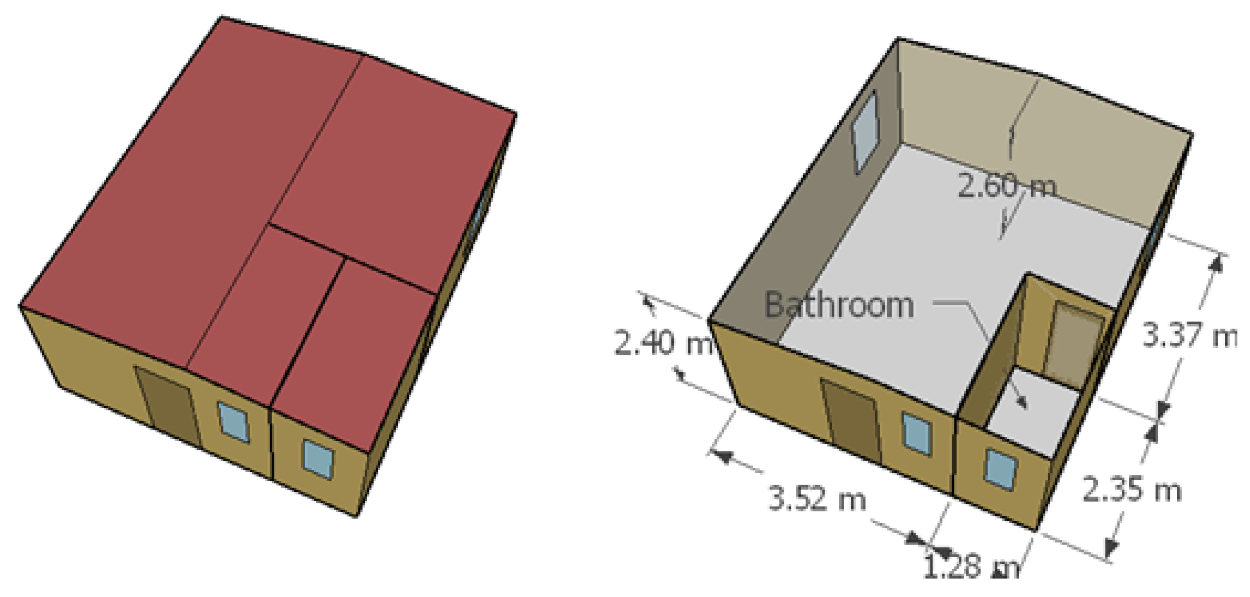
Figure 2.
Two-storey
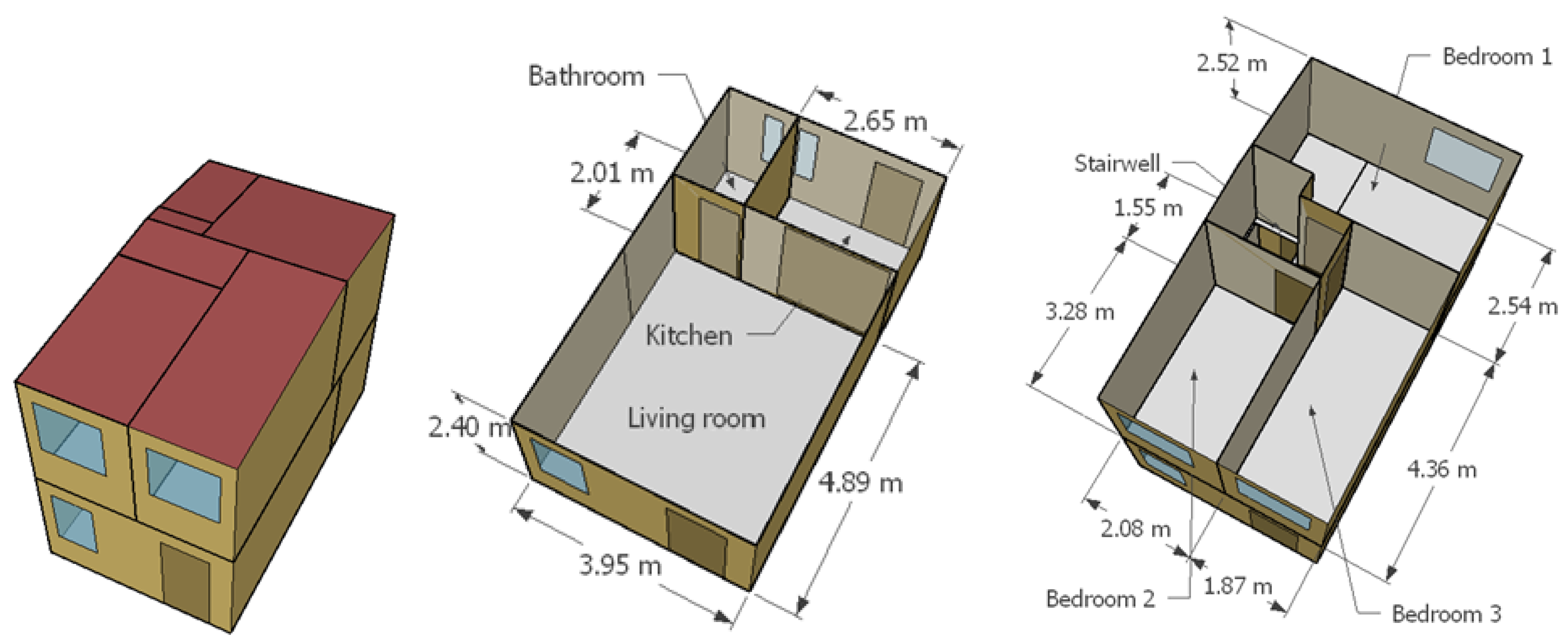
Figure 5.
convergence with r for cooling loads across the four typologies.
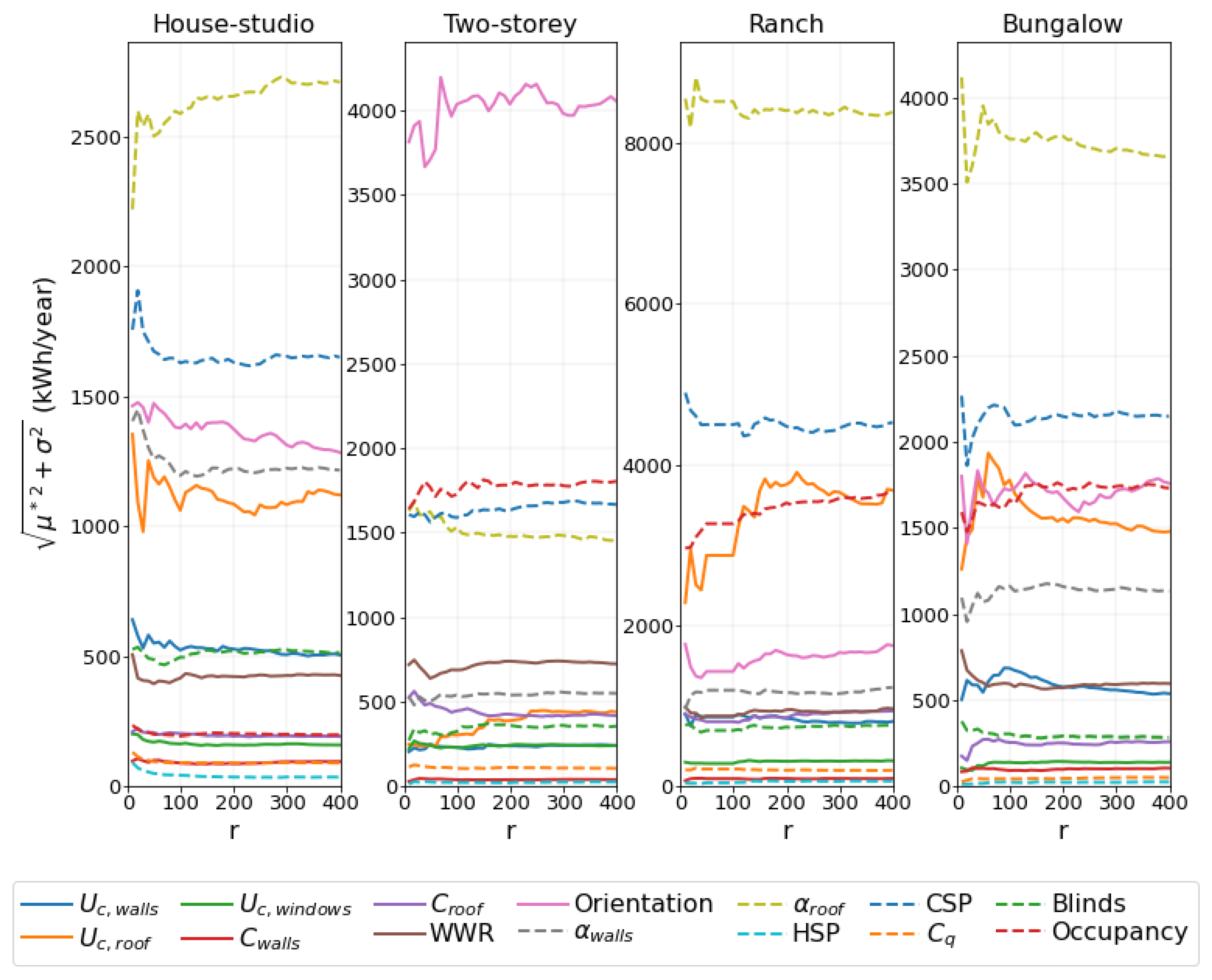
Figure 6.
convergence with r for heating loads across the four typologies.
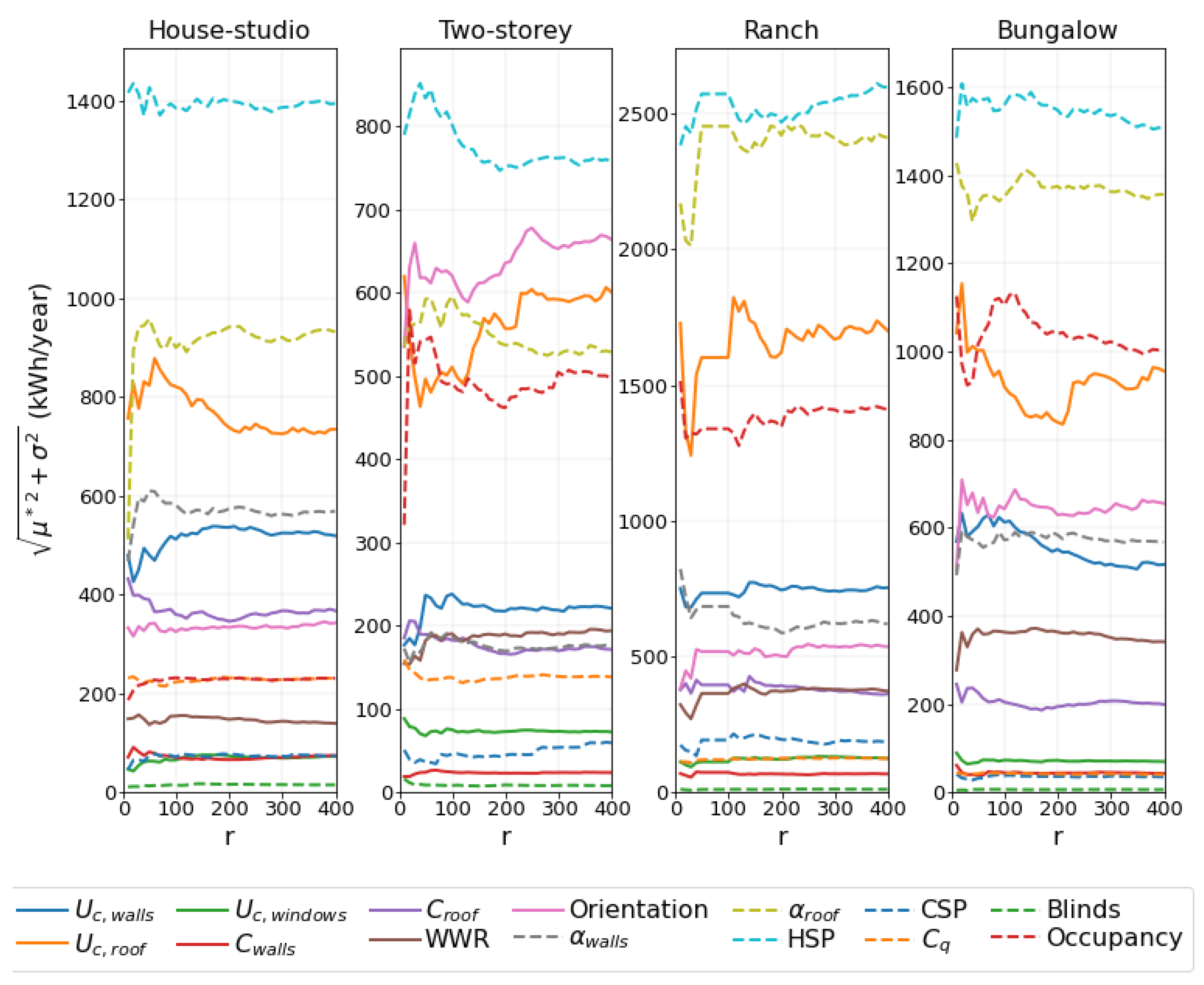
Figure 7.
Relative ranking of the 14 parameters according to their value with respect to the cooling loads after for all investigated p across the four typologies.
Figure 7.
Relative ranking of the 14 parameters according to their value with respect to the cooling loads after for all investigated p across the four typologies.
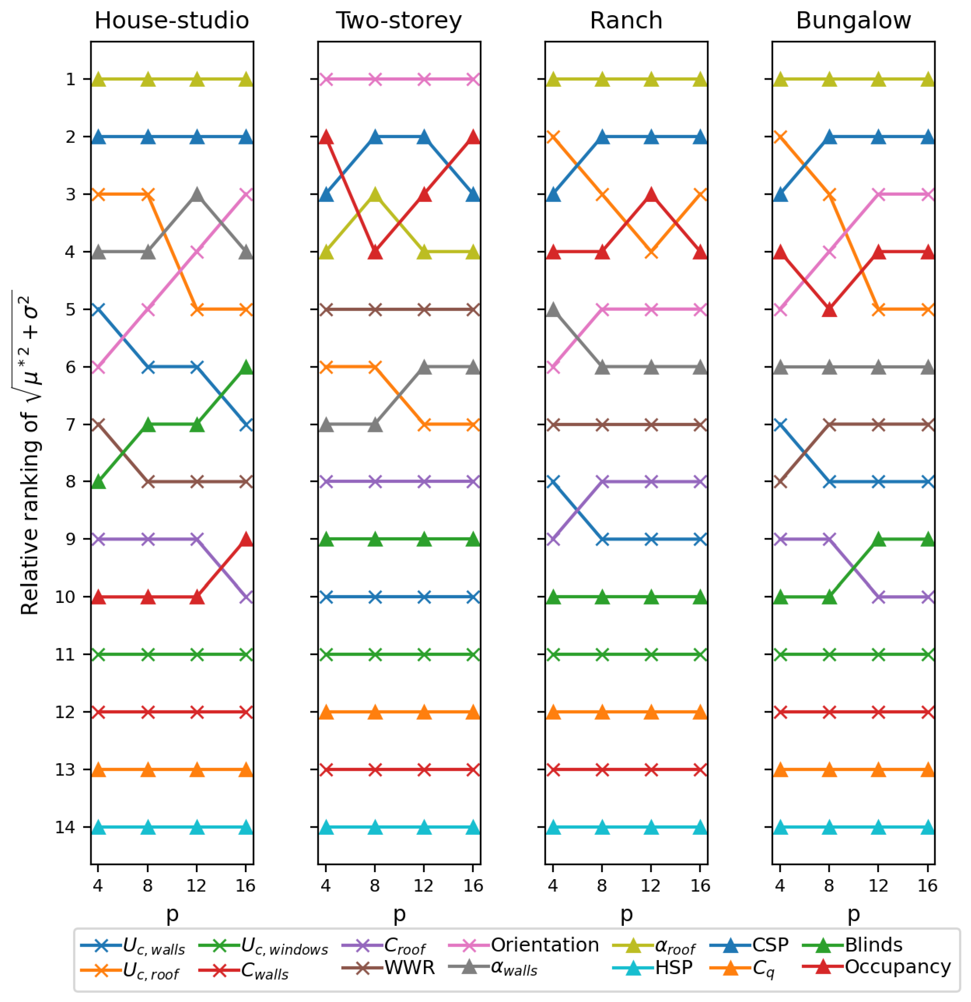
Figure 8.
Relative ranking of the 14 parameters according to their value with respect to the heating loads after for all investigated p across the four typologies.
Figure 8.
Relative ranking of the 14 parameters according to their value with respect to the heating loads after for all investigated p across the four typologies.
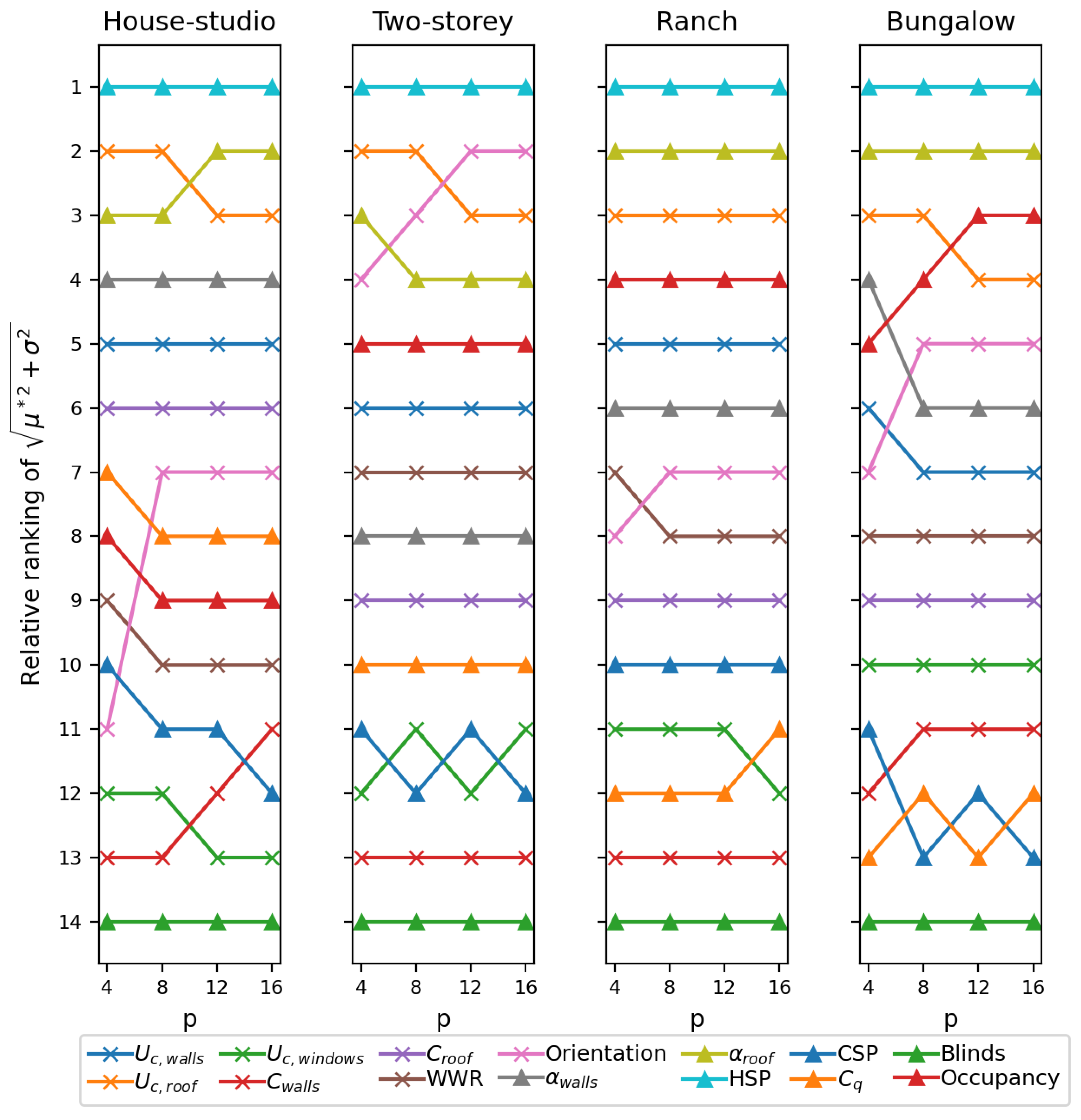
Figure 9.
Morris method resulting and for cooling, heating and total thermal loads for the house-studio typology with and .
Figure 9.
Morris method resulting and for cooling, heating and total thermal loads for the house-studio typology with and .
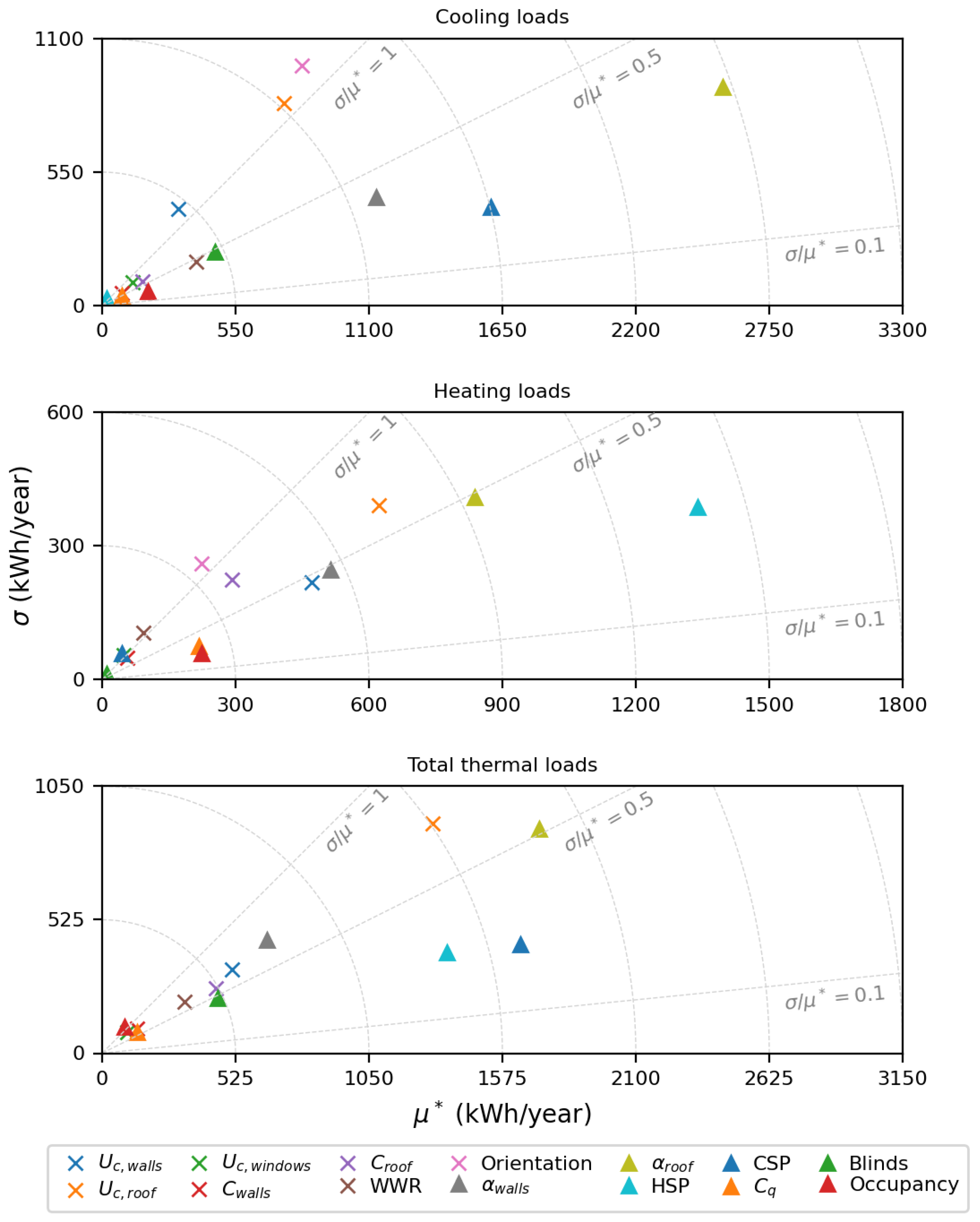
Figure 10.
Morris method resulting and for cooling, heating and total thermal loads for the two-storey typology with and .
Figure 10.
Morris method resulting and for cooling, heating and total thermal loads for the two-storey typology with and .
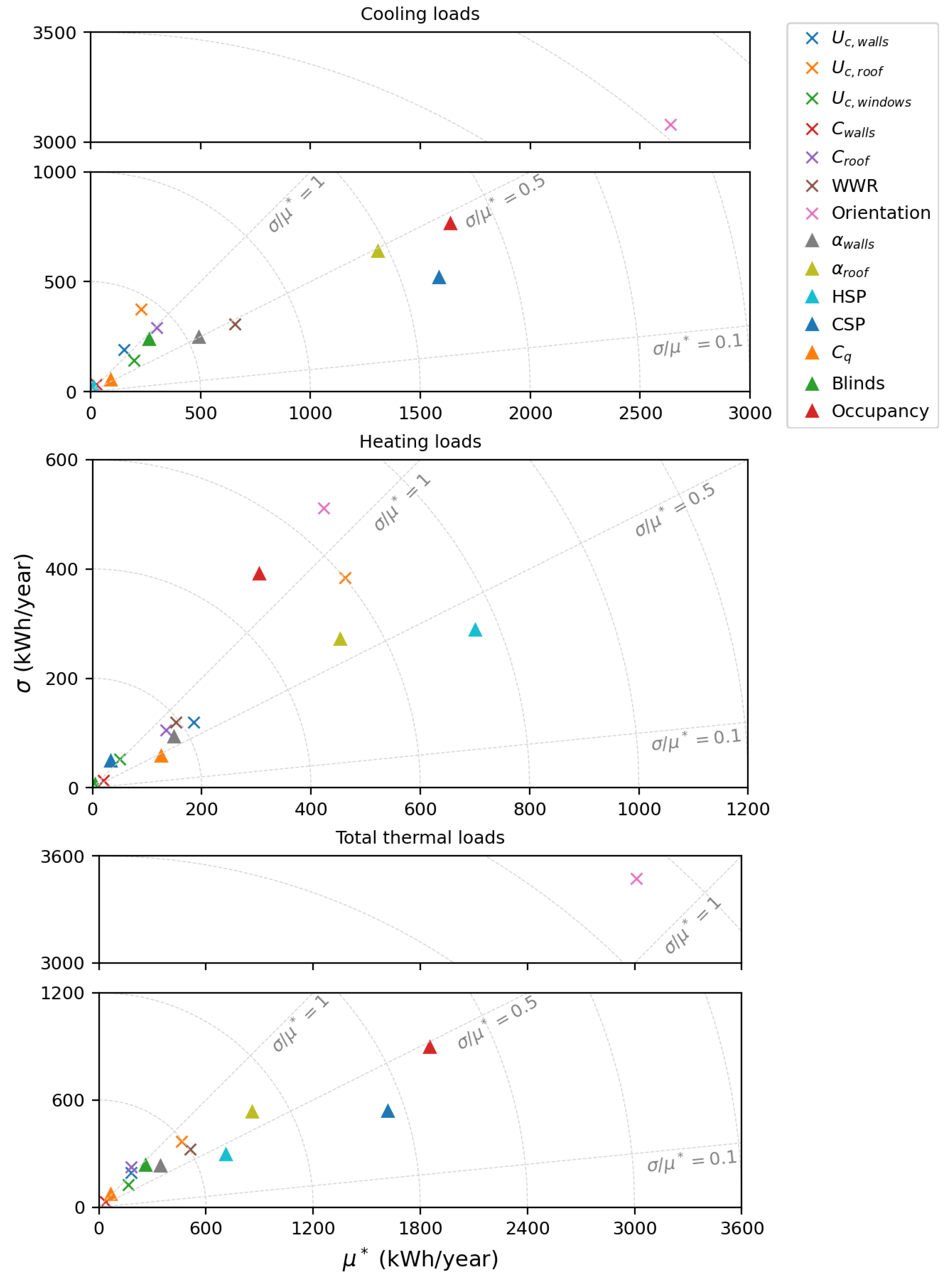
Figure 11.
Morris method resulting and for cooling, heating and total thermal loads for the ranch typology with and .
Figure 11.
Morris method resulting and for cooling, heating and total thermal loads for the ranch typology with and .
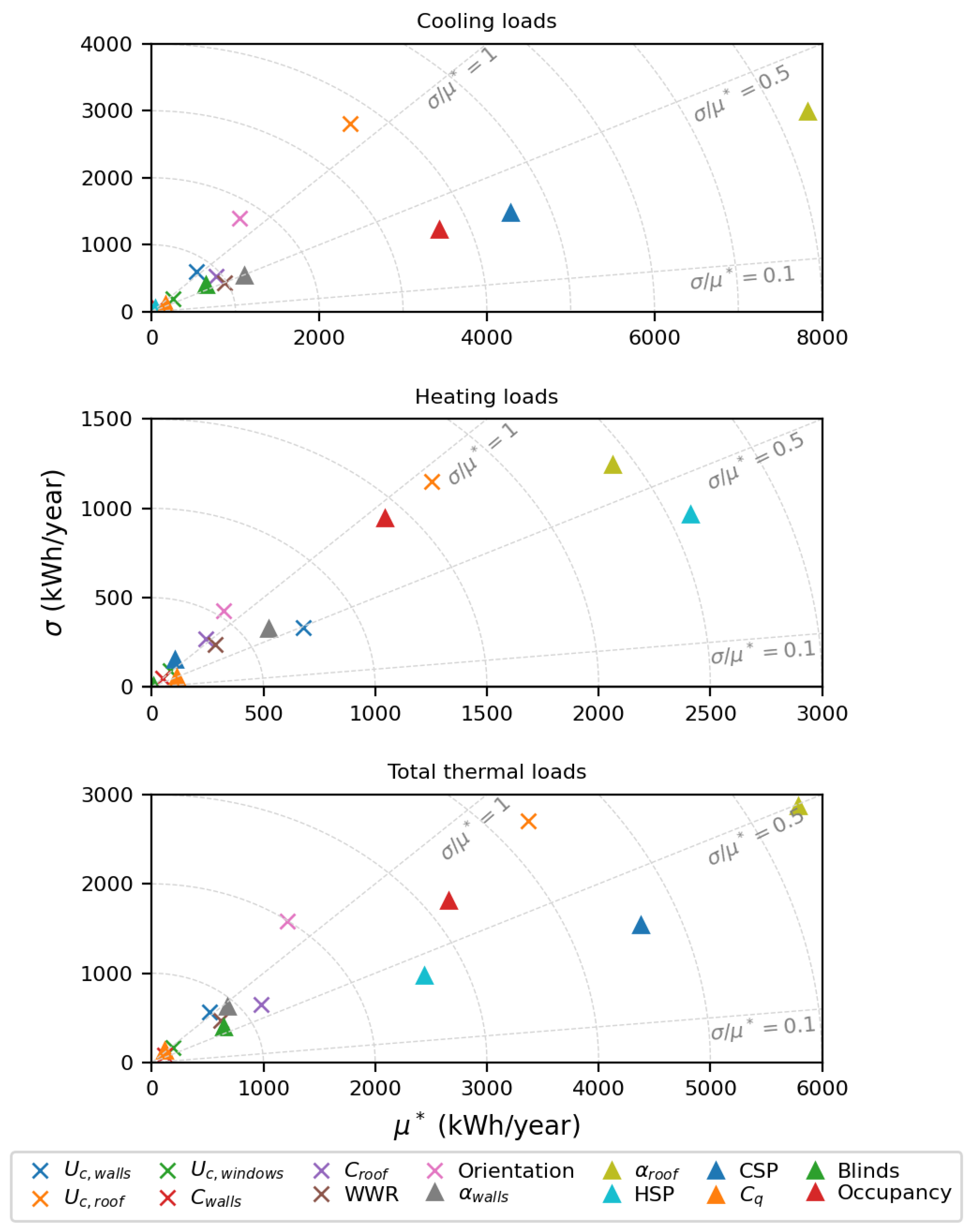
Figure 12.
Morris method resulting and for cooling, heating and total thermal loads for the bungalow typology with and .
Figure 12.
Morris method resulting and for cooling, heating and total thermal loads for the bungalow typology with and .
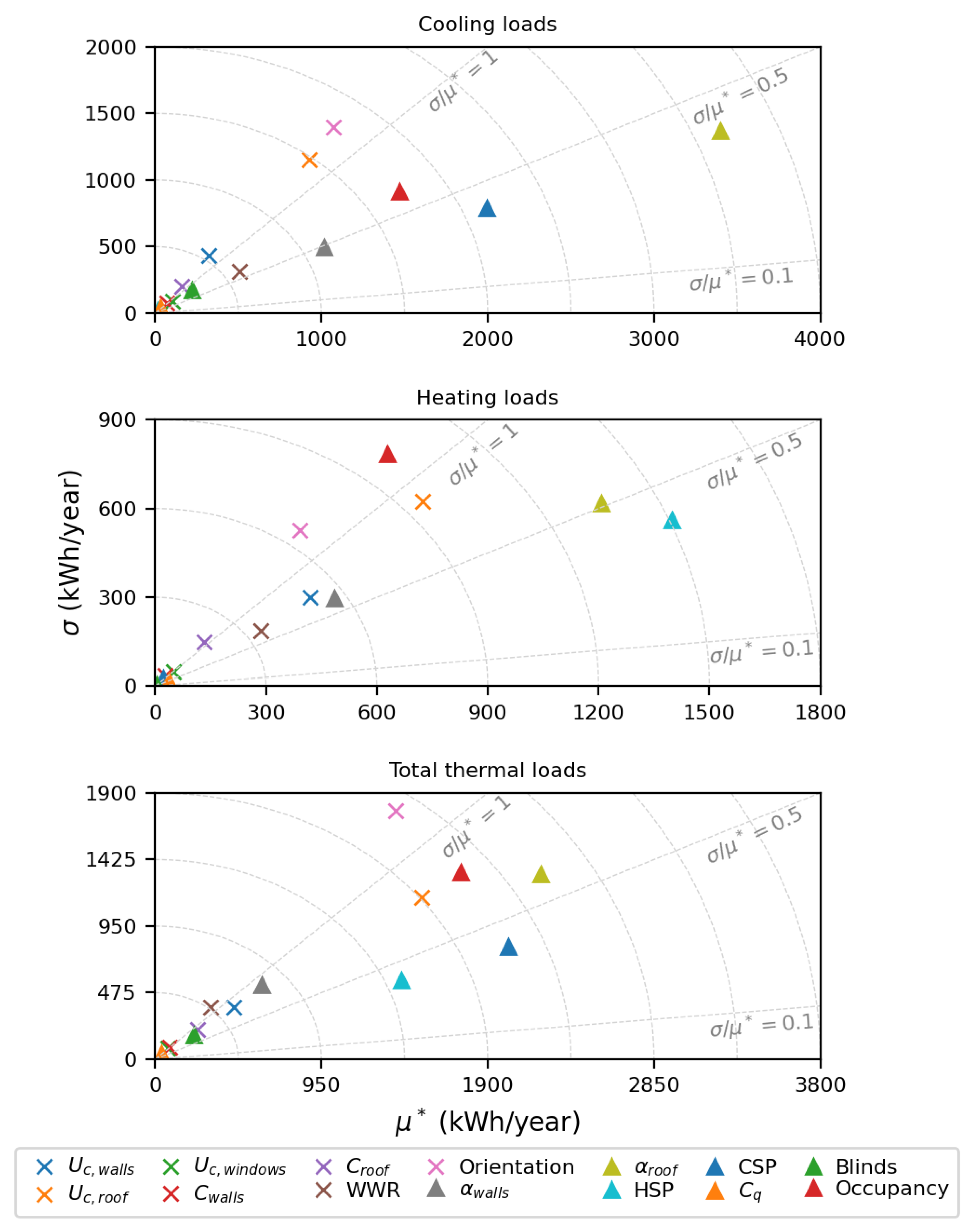

Table 1.
Parameters subject to SA and their ranges.
| Parameter | Acronym | Unit | Min | Max |
|---|---|---|---|---|
| Exterior walls conductance | W/mK | 0.5 | 6.0 | |
| Roof conductance | W/mK | 0.5 | 25.0 | |
| Windows conductance | W/mK | 6.0 | 350.0 | |
| Walls thermal capacitance | kJ/mK | 200 | 400 | |
| Roof thermal capacitance | kJ/mK | 100 | 580 | |
| Window-to-wall ratio | WWR | % | 10 | 30 |
| 15 | 50 | |||
| 10 | 30 | |||
| 5 | 25 | |||
| Front facade orientation | Orientation | º | 0 | 360(p-1)/p |
| Walls solar absorptivity | - | 0.1 | 1.0 | |
| Roof solar absorptivity | - | 0.1 | 1.0 | |
| Heating setpoint | HSP | ºC | 18 | 22 |
| Cooling setpoint | CSP | ºC | 23 | 27 |
| Windows air permeability | g/sm | 0.096 | 0.898 | |
| Windows blinds activation criteria |
Blinds | W/m | 0 | 1000 |
| Occupancy | Occupancy | number of people |
1 | 3 |
| 1 | 7 | |||
| 1 | 15 | |||
| 1 | 8 |
Table 2.
Simulation results ranges for the Morris method samples across the four typologies.
| Cooling (kWh/year) |
Heating (kWh/year) |
Total (kWh/year) |
||
|---|---|---|---|---|
| mean | 2104 | 1282 | 3385 | |
| House-studio | min | 79 | 48 | 815 |
| max | 6201 | 4176 | 7634 | |
| mean | 1876 | 592 | 2468 | |
| Two-storey | min | 175 | 0 | 515 |
| max | 5501 | 2742 | 6174 | |
| mean | 5305 | 1926 | 7231 | |
| Ranch | min | 115 | 21 | 1082 |
| max | 17748 | 8068 | 18746 | |
| mean | 2510 | 1192 | 3701 | |
| Bungalow | min | 36 | 38 | 513 |
| max | 8899 | 4533 | 9363 |
Table 3.
Morris top 5 most relevant parameters for cooling and heating loads across the four typologies.
Table 3.
Morris top 5 most relevant parameters for cooling and heating loads across the four typologies.
| House-Studio | Two-Storey | Ranch | Bungalow | |
|---|---|---|---|---|
| Cooling | Orientation | |||
| CSP | CSP | CSP | CSP | |
| Occupancy | Occupancy | Orientation | ||
| Orientation | Occupancy | |||
| WWR | Orientation | |||
| Heating | HSP | HSP | HSP | HSP |
| Orientation | ||||
| Occupancy | ||||
| Occupancy | ||||
| Occupancy | Orientation |
Disclaimer/Publisher’s Note: The statements, opinions and data contained in all publications are solely those of the individual author(s) and contributor(s) and not of MDPI and/or the editor(s). MDPI and/or the editor(s) disclaim responsibility for any injury to people or property resulting from any ideas, methods, instructions or products referred to in the content. |
© 2024 by the authors. Licensee MDPI, Basel, Switzerland. This article is an open access article distributed under the terms and conditions of the Creative Commons Attribution (CC BY) license (http://creativecommons.org/licenses/by/4.0/).
Copyright: This open access article is published under a Creative Commons CC BY 4.0 license, which permit the free download, distribution, and reuse, provided that the author and preprint are cited in any reuse.


