Submitted:
09 August 2024
Posted:
09 August 2024
You are already at the latest version
Abstract
This paper investigates the energy dissipation level of a nonlinear vehicle suspension system. The suspension system is modelled as a mass-spring-damper system, which is designed using the output frequency response function (OFRF) method. This method enables the derivation of an explicit relationship, between the system output spectrum (or Performance metric) and the system nonlinear parameters of interest. The OFRF polynomial, of the energy dissipation level, was derived in terms of the nonlinear parameters of interest. The results obtained show that the OFRF model, of the energy dissipation level, could be used to estimate the amount of heat dissipated, for a set of design parameters. This has potentials of providing some insights, in the design of vibration-based energy harvesters, as some of the wasted heat energy could be converted to electrical energy.
Keywords:
vibration isolation system
; nonlinear suspension system
; OFRF
; nonlinear systems
; energy dissipation
; nonlinear damping
1. Introduction
To meet the growing needs of modern society, innovative modes of transportation are being developed to improve ride quality, safety and comfort. These improvements are also expected to boost proficiency and ensure cost-effectiveness for all modes of transportation. All ground vehicles experience different levels of vibration, due to irregularities of the road surface. These vibrations are transmitted to the body of the vehicle (including the passengers), through the tyres of the vehicle and the suspension systems (shock absorbers) of the vehicle. Such vibrations can significantly reduce ride comfort, quality and also affect ride stability [1,2,3,4]. In [2], the control of roll and vertical vibrations, of a seat suspension (a two-layer multi-DOF active seat suspension), triggered by the irregular road levels, underneath both sides of the tyres, was investigated. Two controllers, a non-singular terminal sliding mode controller, and an H∞ controller, were employed. The effectiveness of both the seat suspension system and the control techniques employed, were validated using both simulation and experimental analyses. The authors in [3], investigated the impact of asymmetrical damping and geometrical nonlinearities, in the suspension system of a vehicle model, towards ride comfort. It was demonstrated, both numerically and experimentally, that a combination of asymmetric and geometric nonlinearities, improved the ride comfort of passengers, as well as the performance of the suspension system. In [4], an in-wheel vibration absorber, comprising a spring, an annular rubber bushing, and an adjustable damper, whose parameters were determined using an improved particle swarm optimisation (IPSO) algorithm, was proposed for attenuating vibrations generated by the motor. Two control algorithms, a linear quadratic regulator (LQR) and a fuzzy proportional-integral-derivative (PID) approach, were employed to facilitate the control of the suspension damper and the in-wheel damper, respectively. Both methods displayed excellent performance.
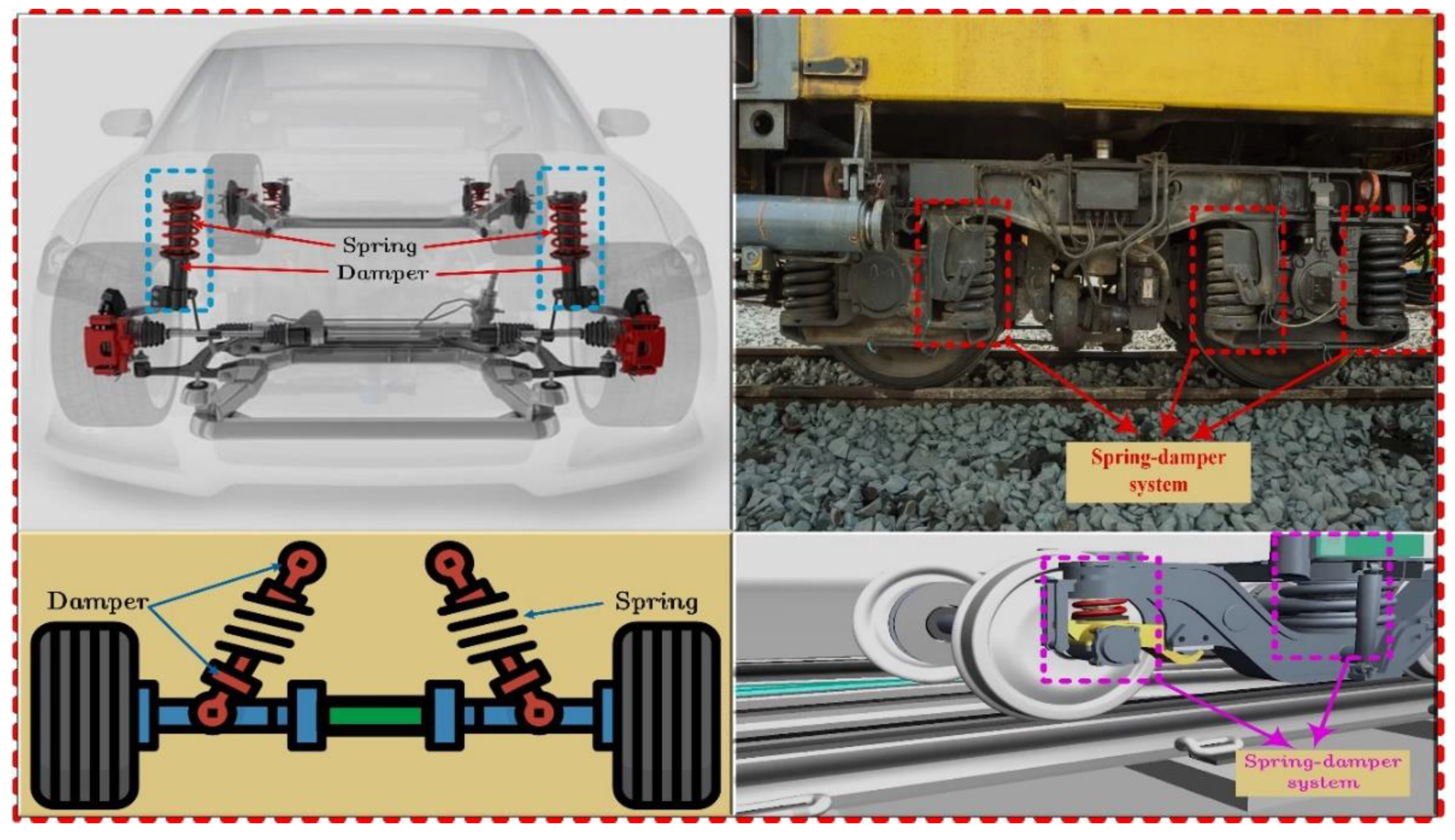
Vehicle suspension systems are designed to curb the effect of adverse ground vibrations and typically comprises a spring, damper and frames/linkages [5]. However, the mass constitutes the body of the vehicle and passengers [5]. A major significance of an isolation spring is its ability to absorb and store energy, from motion bumps and acceleration, with ease. However, isolation springs such as rubber, coil and leaf springs are not capable of dissipating the absorbed energy easily. This can result in unacceptable spring performance before eventual failure, which makes the need for an adequately designed damping system paramount [6]. The damper plays a vital role in the isolation of vibrations from the vehicle’s mass, as it damps out vertical motions by dissipating the transmitted vibration energy as heat energy [6,7]. This ensures the life cycle of the spring is extended and the structural integrity of the system of interest is maintained. The design of a good isolation system is important in vehicle suspension systems to ensure a decent ride comfort [7,8,9]. Lu and his co-authors, in [10], classified nonlinear dampers into three groups namely- nonlinear stiffness dampers, nonlinear-stiffness nonlinear-damping dampers, and nonlinear damping dampers. Based on this classification, the authors reviewed three dampers that are commonly employed in real-world engineering - nonlinear energy sink (NES), particle impact damper (PID), and nonlinear viscous damper (NVD), respectively [10].
Figure 1.
Applications of the suspension system.
Due to the inherent nonlinearity present in all physical shock and vibration isolation systems, more interests have been shown in nonlinear vibration isolation systems. This has led to nonlinear isolation designs of engine mounts being widely reported in literature [11,12,13,14,15].
The authors in [11] compared two models of ride comfort for a multibody dynamic system, based on different damping characteristics - nonlinear damping and its equivalent linear damping. The responses from the driver’s seat were compared using these models and it was revealed that the model based on the nonlinear damping provided a more accurate result compared to that provided by the equivalent damping system. However, in [12], the authors developed a novel nonlinear quasi-zero-stiffness (QZS) vibration isolator, whereby the suspension system was made nonlinear from the geometric arrangement of the inclined springs. The QZS isolator is characterised by a high-static and low-dynamic stiffness. Results obtained showed that the QZS vibration isolator, with its active controller, demonstrated a good isolation performance for large amplitude excitations. The authors in [13] conducted a computational study on a similar model as in [12], which is the QZS isolator. However, for their study, they considered various road profiles as per ISO 8608. The study revealed that the proposed system, reduced about 92% and 88% of external excitations, on an average, in road class B-D and E-H, respectively. The impact of the velocity of a vehicle, with a nonlinear suspension system, on the dynamic behaviour of a Bernoulli-Euler bridge, was investigated in [14]. It was established that the speed of the vehicle, as well as its suspension stiffness and damping characteristics, are the only significant parameters that can influence the dynamic behaviour of a bridge subjected to a moving vehicle. In [15], the influence of asymmetrical damping and geometrical nonlinearities, in the performance of a vehicle’s suspension system, was explored. Numerical and experimental results verified that geometrical nonlinearity significantly impacts the behaviour of the damping and stiffness characteristics of a suspension system, thus, facilitating its ability to minimise vibrations.
Several analytical methods exist for the study of nonlinear suspension systems, such as the harmonic balance methods [16,17], averaging methods [18,19] and describing function methods [20,21]. However, these methods do not clearly reveal the relationship between the vehicle suspension performance metrics and the system’s nonlinear parameters. The frequency-based method, the Output Frequency Response Function (OFRF) method [22,23,24,26], is a systematic frequency domain approach that enables the derivation of the system’s output spectrum, in terms of the nonlinear parameters of interest. This method is employed in the present study, as it facilitates the analysis and design of nonlinear systems, in the frequency domain.
A model for a single degree of freedom (SDOF) passive vibration isolation system, with cubic stiffness and damping characteristics, was studied in [25]. The method of averaging perturbation was used, to observe the effects of nonlinearities, on the dynamic behaviour of the system. The same nonlinear passive mount was also considered by Peng and Lang in [26]. However, the OFRF method was employed in the theoretical analysis of the output frequency response behaviour, with respect to the system nonlinearities and subsequently verified by simulation studies. A similar system was investigated in [27], where the effects of the system nonlinear parameters, on the relative and absolute displacement transmissibility, were explored.
In this study, the vehicle suspension system, shown in Figure 2, and similar to that in the articles [25,26,27], is investigated. However, an analysis and design of the suspension system is conducted, using the OFRF method. Optimal values of the design parameters are obtained for a desired design specification, and the designed parameters are validated using numerical simulations. Furthermore, for the first time, the energy dissipation performance, of a vehicle suspension system, is investigated using the OFRF method. The effects of the nonlinearities of the designed suspension system, on the energy dissipated by the isolation system, is explored. An investigation is then performed using the OFRF method, where the nonlinear system parameters are designed, for a desired energy dissipation level, of the suspension system.
The rest of the paper are organised as follows: Section 2 provides the model formulation of the suspension system to be investigated; Section 3 introduces the OFRF method, while Section 4 describes the determination of the OFRF representation, for the system output spectra; Section 5 presents the system design and optimisation process for a desired design specification, while Section 6 demonstrates, with numerical simulations, the effects of the system parameters; Section 7 analyses the energy dissipation level of the designed suspension system, as well as the effects of system nonlinearities on the dissipation level; Conclusions are reached in Section 8.
2. Model Formulation
A schematic diagram of the nonlinear Single degree of freedom (SDOF) suspension system, considered in this study, is shown in Figure 2. This includes a suspended oscillating sprung mass, , representing the quarter mass of a vehicle body, with an absolute displacement of , due to a base motion of y(t). The suspension system has two
nonlinear isolation components comprising nonlinear damping (c1, c2) and nonlinear stiffness elements.
Figure 2.
Schematic of the nonlinear suspension system under a base excitation.
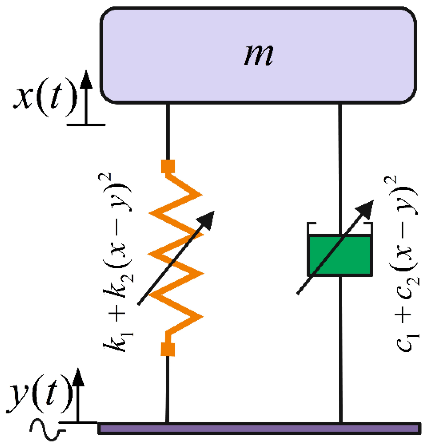
The equation of motion for the suspension system is given by
where is the relative displacement between the base and the sprung mass, while and are the damping and stiffness functions, respectively. However, the damping and stiffness functions are described as
Assuming the base excitation is harmonic, that is
then system (1) becomes
where and are the excitation frequency and amplitude of the base displacement, respectively, while is the force transmitted through the vibration isolation system (a parallel combination of the spring and damper elements).
To ensure ride comfort, the minimisation of the transmitted force is required. The transmitted force output spectrum is maximum at the resonant frequency,. Consequently, becomes the frequency of interest and the objective will be to minimise , at the resonant frequency. The procedure outlined by Zhu and Lang in [28], for the analysis and design of a SIMO system, using the OFRF method, will be employed here.
In the next section, the OFRF method will be introduced, considering a general Volterra system, described by a nonlinear differential equation.
3. The Output Frequency Response Function (OFRF)
The differential equation presented in Equation (5) is used to describe a class of Volterra systems
where, is the maximum degree of nonlinearity, with respect to the input and output parameters of the system, and is the order of the derivative. Conforming to the OFRF method [22,23,24,26], the output frequency response, of the system described in Equation (5), can be characterised by a polynomial function, in terms of the system nonlinear parameters as
where, are the maximum order of , for , in the output spectrum , of the system described by the polynomial in Equation (6). The system of symbols, are frequency functions, which are also referred to as the OFRF coefficients. These functions are complex values and are dependent on the system’s input and linear characteristic parameters, where and . Furthermore, is a set of monomials and also known as the OFRF structure. They are derived in terms of the nonlinear characteristic parameters of the system. It should be noted that represents the coefficients of , with the same dimension, and needs to be evaluated in order to obtain the OFRF representation of system (5). However, the monomials need to be determined, first, using a recursive algorithm proposed in Peng et al. [26]. For a Single-Input-Multiple-Output (SIMO) system, an elaborate procedure has been described by Zhu and Lang in [28]. Let the set of monomials, in the OFRF representation of the nth-order output spectrum, be denoted as and the frequency function vector, be denoted as , then the OFRF can be described as
Where
Here, the monomials, can be determined using [26]
Where
The symbol ‘’ is the Kronecker product.
Then the set of monomials can be obtained as
In Section 4, the OFRF method will be used to derive an analytical relationship, between the output spectra of system (4) and its nonlinear parameters of interest. Thereafter, a system analysis and design will be conducted, in order to obtain the optimal nonlinear parameters for the desired performance metrics, based on design specifications. The effects of the nonlinear parameters, and, on the system output spectra, are also explored using numerical simulations.
4. Determination of the OFRF Representation
In this section, the OFRF representation of the output spectra of system (4) is obtained in terms of the nonlinear parameters of interest, and. As indicated in Equation (6), the OFRF of the nonlinear system (5), is a polynomial function of the nonlinear characteristic parameters of the system. The coefficients of the OFRF are the functions of the output frequency of the system, determined by the specific structure of Equation (5), the system input spectrum, and the linear characteristic parameters of the system. To enable the use of the OFRF representation of system (4), for system analysis and design, its coefficients and monomials have to be determined first. The following analyses have been performed, using the system parameters presented in Table 1.
It can be inferred that the system in Equation (4), is the instance of system (5), with , , , , , , else .
4.1. Determination of the OFRF Monomials
To determine the OFRF representation, the algorithm described in [26], as well as in [28], for SIMO systems, is employed. The recursive algorithm therein, is applied to system (4), to determine the set of monomials, , up to the N = 7th order, which yields
It should be noted, that the same set of monomials is obtained for both outputs of system (4). This implies that the OFRF of the outputs of system (4), can be expressed as
where and are the OFRF coefficients of the output spectra of system (4), and respectively. Next, the OFRF coefficients are determined.
4.2. Determination of the OFRF Coefficients
To determine the coefficients of the OFRFs for the system outputs, and , the steps outlined in [22,23,24,26,28] are followed. The least square approach is used to determine and as
where,
and
and represents the output spectra of system (4), when and , for , where for a varied set of N.s.m−3 and N.m−3. Therefore, considering N=7, the OFRF representations of the output spectra of system (4) can be expressed as
Given the output spectra, in terms of the nonlinear parameters of interest, as in Equation (15), parameter optimisation can be easily conducted. For example, for the resonant frequency, which is the frequency of interest, and given as , the OFRF representations of the system output spectra, at the frequency of interest, are determined as
and
respectively.
In this case, the magnitude of the output spectra, and , of system (4), are plotted for a varied set of N.s.m−3 while keeping fixed, as presented in Figure 3.
The results, as presented in Figure 3, are obtained using the OFRF models, of the output spectra, as given in Equations (16) and (17) respectively, and compared with results obtained from numerical simulations. Note that some of these results have been achieved for parameters beyond those used to determine the OFRF representations. The outcome shows a good match, between the OFRF-based results and results obtained from numerical simulations.
This indicates the usefulness of the OFRF method and, as revealed, it also shows that it provides a good representation of the actual system output spectra. The implication of this is that the OFRF representations, of the output spectra of system (4), can be used for the analysis and design of the system output spectra. This is because, in using the OFRF, an explicit association of the system performance metrics, with the system design parameters, can be established.
It should be noted that a poor OFRF representation of the actual system output spectra, will provide poor analytical results. Such poor representations can be as a result of large numerical errors generated during the determination of the OFRF coefficients. This typically occurs when the parameters are chosen to be large values, with large numerical difference among them, and also when the set of parameters selected, cover a wide range. This will cause the values of the elements in the matrix , to be extremely large. Computational errors may result when the inverse of matrix is computed in MATLAB. Such a problem can be solved by following the steps described in [23,28].
5. System Optimisation
The objective now is to minimise the unwanted force transmitted at the resonant frequency, through the isolation elements (spring-damper system), to an acceptable limit. Let be the acceptable threshold of the force transmitted through the vibration isolator, then the optimisation problem can be formulated as
Using the OFRF of Equation (17), the relationship between the design parameters, and , and the output spectrum, , is established and provided in Figure 4 and Figure 5. Looking at Figure 5, it is apparent that the contour map can be used as a design guide. The results of two design specifications are presented in Table 2. To determine the actual output response, , the designed parameters are substituted into the system model (4), and simulated, numerically, using the MATLAB Runge-Kutta 4 algorithm.
It should be noted that the second design specification was achieved, for parameter values beyond the range of parameters used to determine the OFRF, i.e., N.s.m−3 and N.m−3. In Table 2, it is observed that the actual output responses, obtained using the designed parameters, and , clearly matches the specified output responses, with insignificant percentage errors. This reaffirms the effectiveness of the OFRF-based optimal design.
Looking at the time histories of the force transmitted at the resonant frequency in Figure 6, it is obvious that the designed nonlinear vibration isolation system, performs better compared to its corresponding linear counterpart (where the nonlinear characteristic parameters, ). Moreover, a close observation of the time-history of the transmitted force, due to the designed nonlinear isolation system, reveals that the desired transmitted force, at the resonant frequency, is achieved. It should be noted that minimising the force transmitted along the isolation elements, to an acceptable threshold, , results in a decrease in the system output spectrum, .
Furthermore, though the system design has been performed at the resonant frequency, it is imperative to verify that the designed nonlinear optimal parameters, maintain the same performance on the system output spectrum, across the entire frequency range. This is verified in Figure 7 which compares the performance of the nonlinear design, to its corresponding linear counterpart (i.e., when ), on the system output spectrum. It is apparent that not only do the designed optimal parameters achieve a specified output spectrum, at the resonant frequency, they are also adequate at suppressing the vibration levels over other frequencies.
The above system analysis and design have been performed using the OFRF method. It is evident that this method facilitates a systematic analysis and design of nonlinear Volterra systems, compared to other methods. The next section shows the individual effect of the system parameters, on the output spectra of the system, considered in this study. Each parameter is varied while fixing others. These have been performed using numerical simulations.
6. Numerical Studies
To demonstrate the effects of , , and , on the output spectra of system (4), numerical studies were performed, and the corresponding results are presented in Figure 8, Figure 9 and Figure 10, respectively. Figure 8 shows the well-known influence of linear damping characteristic parameter, on the output spectra of system (4), where a good isolation performance is witnessed over the resonant region. However, its detrimental effect, over the region where isolation is required (), when high damping level is employed, suggests the need for the integration of a nonlinear damping element. In Figure 9, the effect of is evident around the resonant region. It is apparent that as increases, the resonant frequency, , is increased beyond the natural frequency; however, its harmful effect (instability) is controlled by an increased damping characteristic. Besides, the effect of increasing the nonlinear viscous damping characteristic parameter, , is observed in Figure 10, to suppress the vibration at the resonant region. Meanwhile, the vibration response, at the non-resonant regions (i.e., at low and high frequency ranges), remain unaffected.
7. Energy Dissipation Analysis
For the SDOF system described in Figure 2, the vibration isolation elements (spring and damper), experience energy loss due to their dissipative characteristics. The power dissipated at any instant is , and the energy lost over one complete cycle, , is given as
Let the relative displacement, , then . Equation (19) becomes
which yields
where and It is observed, from Equation (21), that the energy dissipated by the suspension system is, mainly, due to its damping characteristics. However, it should be recalled, as seen in Equation (16), that is a function of both nonlinear damping, and nonlinear stiffness, . The OFRF of the energy lost by the suspension system, over one complete cycle, can be derived by substituting Equation (15a) into Equation (21), which yields
Equation (22) indicates is a function of , , , and the design parameters, and . This indicates that the OFRF, of the energy dissipated, can be derived in terms of the design parameters.
Just as the OFRF representation of the output spectrum, , of system (4), was determined and presented in Equation (15a), the OFRFs of the squared and quartic magnitudes of , are also derived as
where N = 7, while and are functions of frequency, and represent the OFRF coefficients of and , respectively. Substituting Equation (23) into Equation (22) yields
Equation (24) indicates that an estimate of the energy dissipated, per cycle, by the suspension system, can be determined for a set of design parameters. The relationship between the energy dissipation and the design parameters, at the resonant frequency, , is provided in Figure 11. It is seen, in Figure 12, that a large amount of energy is dissipated when a linear vibration isolator is used (when ). However, the energy dissipated reduces with the integration of nonlinear damping and stiffness characteristics. This behaviour is due to the impact of the nonlinear components, on the relative displacement of the suspension system. The relative displacement decreases as the nonlinearities increase, which, consequently, reduces the force transmitted and energy dissipated, by the suspension system. It is also evident that the energy dissipation level is very sensitive to the nonlinear damping characteristic, and less sensitive to the nonlinear hardening stiffness characteristic. Surface plots between the energy dissipated by the suspension system and the design parameters, beyond the resonant region, that is, at and , are presented in Figure 13 and Figure 14, respectively.
Besides, Equation (24), which is the OFRF of the energy dissipation of the suspension system, can be used to estimate the energy dissipated, for a set of optimal design parameters, and . An estimation guide can be developed using an OFRF-generated contour map which can facilitate the selection of design parameters for a specified energy dissipation level, as illustrated in Figure 15.
Choosing N.m−3, along the contour line of 20J, gives a corresponding nonlinear damping value of N.s.m−3. Substituting and into system (4) and solving for the energy dissipation level, numerically, yields a value of 21.08J, which matches the design requirement well, with a percentage error of -5.1%.
The results from numerical studies, to show the individual effects of the system parameters, , and , on the energy dissipation level of the suspension system, over the entire spectrum, are presented in Figure 16, Figure 17 and Figure 18, respectively. This was done by varying either one of the parameters, , or , while keeping the other two fixed. In Figure 16, the unwanted impact of linear damping, over the high frequency region, experienced by the output spectra of system (4), is also apparent for the energy dissipation spectra. It is seen that while an increase in linear damping reduces the energy dissipation, over the resonant region, it increases the energy dissipation, significantly, across the non-resonant regions. Likewise, increasing the nonlinear damping, minimises the energy dissipation, at the resonant region. However, unlike the linear damping, the corresponding increase in the energy dissipation, in the non-resonant regions, is far less significant, as illustrated in Figure 17.
The influence of hardening stiffness, as shown in Figure 18, is similar to the effect it has on the output spectra of system (4). In this case, as nonlinear stiffness is increased, the resonant peak of the energy dissipation level, is reduced at . This is due to the resonant-shift effect of , on the resonant energy, beyond the natural frequency.
Using the OFRF representations derived, the variations of both the energy dissipated and force transmitted by the suspension system, as a function of the nonlinear stiffness parameter, , are shown in Figure 19. It is observed that while the force transmitted by the suspension system, is less sensitive to , the sensitivity of the energy dissipated, to , is insignificant. This reaffirms the deduction made from Figure 12. This deduction is largely because the spring element stores potential energy when compressed/stretched, and dissipates insignificant amounts of energy. It is also seen that for a fixed , increasing , causes an insignificant decrease in the energy dissipated per cycle. However, the vibration force transmitted is increased. Similarly, the results illustrated in Figure 20, are the variations of both the energy dissipated and force transmitted, by the suspension system, as a function of the nonlinear damping parameter, . In this case, it is apparent that both performance metrics are significantly sensitive to . Both performance metrics also, progressively, decrease as increases. This is because the relative displacement of the vehicle suspension system, decreases as increases, and this causes a decrease in both the force transmitted, and energy dissipated, by the suspension system.
Illustrated in Figure 21, is the variation of the suspension damper force, , and the energy dissipated by the suspension system, , with increase in excitation frequency. It is observed that both quantities attain maximum values at the resonant frequency . This is expected as a high damping force is required at resonance (i.e., region of maximum displacement), which corresponds to a high energy dissipation level, by the suspension system. However, the energy dissipation, beyond resonance, is significantly low, with respect to the level of damping force, compared to other frequency regions. This is due to the low relative displacement experienced at high frequencies.
Four hysteretic curves (A, B, C, and D), are presented in Figure 22, from different combinations of the designed nonlinear parameters of system (4). For a vibration isolation system, the area of the Force-displacement curve (), gives an indication of the energy dissipated per cycle, by the isolation system, at any frequency of interest (typically the resonant frequency). It is observed that the hysteretic curves C and D, show a smaller displacement span, compared to A and B. This is evidently due to the contribution of the nonlinear damping characteristic, integrated in the suspension systems of C and D. Those of A and B possess a linear damping characteristic only. Nonlinear dampers exhibit a superior vibration isolation performance compared to the corresponding linear case (when ). The presence of a nonlinear damping characteristics, results in the decrease in the magnitude of the relative displacement, .
It should be noted that, compared to linear dampers, nonlinear dampers dissipate, significantly, more amount of heat energy, for an equal amount of excitation [29]. However, such a comparison has not been considered here. Furthermore, while for a linear suspension system configuration, the hysteretic curve assumes an elliptic shape, this is not the case for a nonlinear suspension system.
As observed in Figure 23, the effect of , on curves C and D, with intercept , on the vertical axis, is apparent, compared to the curves A and B (with intercept, ), without the effect of . This is seen to be as a result of the influence of , on the system output response, , which is a function of the nonlinear damping characteristics,.
8. Conclusions
In this study, the vibration isolation performance, of a nonlinear vehicle suspension system, modelled as a SDOF vibration isolation system, was investigated. The Output Frequency Response Function (OFRF) method was the analytical tool employed, for the analysis and design of the suspension system, based on the design criteria. This method was used because of its ability to explicitly express the system performance metrics, in terms of the design parameters of interest. The results obtained, from the analytical and simulation studies, demonstrate the effectiveness of this method, in the analysis and design of vibration isolation systems. To demonstrate the extensive effects of the designed nonlinear system parameters, a comparative study was conducted, between the nonlinear system model and the corresponding linear system (where the nonlinear components are fixed to zero). The outcome reveals the influence of the system nonlinearities, especially at the resonant region, as the resonant peak is largely reduced without a detrimental effect at higher frequencies. This demonstrates the superior vibration isolation capability, of nonlinear vibration isolation systems, compared to their linear equivalent.
Furthermore, the energy dissipated per cycle, by the designed suspension system, was also investigated, using the OFRF method. By employing the OFRF method, a relationship between the Energy dissipation level, of the nonlinear suspension system, and the design parameters, was derived. This polynomial relationship facilitated the estimation of an energy dissipation level, for a set of system nonlinear parameters. The results obtained confirmed the advantage of nonlinear suspension systems, over its linear counterparts. Numerical studies were conducted to demonstrate the effects of nonlinear system parameters, on the energy dissipation level of the suspension system.
Finally, the energy dissipation level of the suspension system, was investigated, using hysteretic curves. The effect of the system nonlinear parameters, on the shape of the hysteresis loop, was explored. The sensitivity of the energy dissipation level, to the nonlinear damping characteristic, compared to the nonlinear stiffness characteristic, was evident. The results in this study reaffirm the vibration suppression advantage of nonlinear suspension systems, over the corresponding linear counterpart.
Author Contributions
Conceptualization, U.D.; methodology, U.D., R.G., Y.Z.; software, U.D; formal analysis, U.D.; investigation, U.D.; writing—original draft preparation, U.D.; writing—review and editing, Y.Z., R.G.; visualization, U.D.; project administration, U.D. All authors have read and agreed to the published version of the manuscript.
Funding
This research received no external funding.
Data Availability Statement
Not applicable.
Conflicts of Interest
The authors declare no conflict of interest.
References
- Cai, L. W. (2016). Fundamentals of mechanical vibrations. John Wiley & Sons.
- Borowiec, M., Sen, A. K., Litak, G., Hunicz, J., Koszałka, G., & Niewczas, A. (2010). Vibrations of a vehicle excited by real road profiles. Forschung im Ingenieurwesen, 74(2), 99-109.
- Soliman, J. I., & Ismailzadeh, E. (1974). Optimization of unidirectional viscous damped vibration isolation system. Journal of sound and vibration, 36(4), 527-539. [CrossRef]
- Liu, M., Gu, F., & Zhang, Y. (2017). Ride comfort optimisation of in-wheel-motor electric vehicles with in-wheel vibration absorbers. Energies, 10(10), 1647. [CrossRef]
- Arana, C., Evangelou, S. A., & Dini, D. (2014). Series active variable geometry suspension for road vehicles. IEEE/ASME transactions on mechatronics, 20(1), 361-372. [CrossRef]
- Alleyne, Andrew, and J. Karl Hedrick. “Nonlinear adaptive control of active suspensions.” IEEE transactions on control systems technology 3, no. 1 (1995): 94-101. [CrossRef]
- Deringöl, A. H., & Güneyisi, E. M. (2021, December). Influence of nonlinear fluid viscous dampers in controlling the seismic response of the base-isolated buildings. In Structures (Vol. 34, pp. 1923-1941). Elsevier. [CrossRef]
- Kumar, S., Medhavi, A., & Kumar, R. (2021). Optimization of nonlinear passive suspension system to minimize road damage for heavy goods vehicle. Int. J. Acoust. Vib, 26(1), 56-63. https://link.gale.com/apps/doc/A659376667/AONE?u=anon~b7686b90&sid=googleScholar&xid=fdd7cfc4.
- Tiwari, V., Sharma, S. C., & Harsha, S. P. (2022). Ride comfort analysis of high-speed rail vehicle using laminated rubber isolator based secondary suspension. Vehicle System Dynamics, 1-27. [CrossRef]
- Lu, Z., Wang, Z., Zhou, Y., & Lu, X. (2018). Nonlinear dissipative devices in structural vibration control: A review. Journal of Sound and Vibration, 423, 18-49. [CrossRef]
- He, S., Chen, K., Xu, E., Wang, W., & Jiang, Z. (2019). Commercial vehicle ride comfort optimization based on intelligent algorithms and nonlinear damping. Shock and Vibration, 2019. [CrossRef]
- Wei, C. (2023). Design and Analysis of a Novel Vehicle-Mounted Active QZS Vibration Isolator. Iranian Journal of Science and Technology, Transactions of Mechanical Engineering, 1-11. [CrossRef]
- Suman, S., Balaji, P. S., Selvakumar, K., & Kumaraswamidhas, L. A. (2021). Nonlinear vibration control device for a vehicle suspension using negative stiffness mechanism. Journal of Vibration Engineering & Technologies, 1-10. [CrossRef]
- Shafiei, B. (2021). Investigating the impact of the velocity of a vehicle with a nonlinear suspension system on the dynamic behavior of a Bernoulli–Euler bridge. SN Applied Sciences, 3(3), 293. [CrossRef]
- Fernandes, J. C. M., Gonçalves, P. J. P., & Silveira, M. (2020). Interaction between asymmetrical damping and geometrical nonlinearity in vehicle suspension systems improves comfort. Nonlinear Dynamics, 99(2), 1561-1576. [CrossRef]
- Borowiec, M., Litak, G., & Friswell, M. I. (2006). Nonlinear response of an oscillator with a magneto-rheological damper subjected to external forcing. Applied Mechanics and Materials, 5, 277-284. [CrossRef]
- Jones, J. P. (2003). Automatic computation of polyharmonic balance equations for nonlinear differential systems. International Journal of Control, 76(4), 355-365. [CrossRef]
- Elliott, A. M., Bernstein, M. A., Ward, H. A., Lane, J., & Witte, R. J. (2007). Nonlinear averaging reconstruction method for phase-cycle SSFP. Magnetic resonance imaging, 25(3), 359-364. [CrossRef]
- Stanzhitskii, A. N., & Dobrodzii, T. V. (2011). Study of optimal control problems on the half-line by the averaging method. Differential Equations, 47, 264-277. [CrossRef]
- Xing, X. N., & Zhang, D. M. (2010). Realization of Nonlinear Describing Function Method Virtual Experiment System Based on LabVIEW. In International Conference of China Communication (ICCC2010). https://file.scirp.org/pdf/31-3.38.pdf.
- Attari, M., Haeri, M., & Tavazoei, M. S. (2010). Analysis of a fractional order Van der Pol-like oscillator via describing function method. Nonlinear Dynamics, 61, 265-274. [CrossRef]
- Lang, Z. Q., Billings, S. A., Yue, R., & Li, J. (2007). Output frequency response function of nonlinear Volterra systems. Automatica, 43(5), 805-816. [CrossRef]
- Jing, X. J., Lang, Z. Q., & Billings, S. A. (2008). Output frequency response function-based analysis for nonlinear Volterra systems. Mechanical systems and signal processing, 22(1), 102-120. [CrossRef]
- Jing, X. J., Lang, Z. Q., Billings, S. A., & Tomlinson, G. R. (2006). The parametric characteristic of frequency response functions for nonlinear systems. International Journal of Control, 79(12), 1552-1564. [CrossRef]
- Jazar, G. N., Houim, R., Narimani, A., & Golnaraghi, M. F. (2006). Frequency response and jump avoidance in a nonlinear passive engine mount. Journal of Vibration and Control, 12(11), 1205-1237. [CrossRef]
- Peng, Z. K., & Lang, Z. Q. (2008). The effects of nonlinearity on the output frequency response of a passive engine mount. Journal of Sound and Vibration, 318(1-2), 313-328. [CrossRef]
- Milovanovic, Z., Kovacic, I., & Brennan, M. J. (2009). On the displacement transmissibility of a base excited viscously damped nonlinear vibration isolator. Journal of Vibration and Acoustics, 131 (5). [CrossRef]
- Zhu, Y., & Lang, Z. Q. (2017). Design of nonlinear systems in the frequency domain: an output frequency response function-based approach. IEEE Transactions on Control Systems Technology, 26(4), 1358-1371. [CrossRef]
- Denoël, V., & Degée, H. (2002). Analysis of linear structures with nonlinear dampers. In Proceeding of the Eurodyn Conference 2002. https://orbi.uliege.be/handle/2268/13026.
Figure 3.
Comparison between the OFRF and numerical simulation results, for (a) and (b) , output spectra of system (4), respectively. .
Figure 3.
Comparison between the OFRF and numerical simulation results, for (a) and (b) , output spectra of system (4), respectively. .
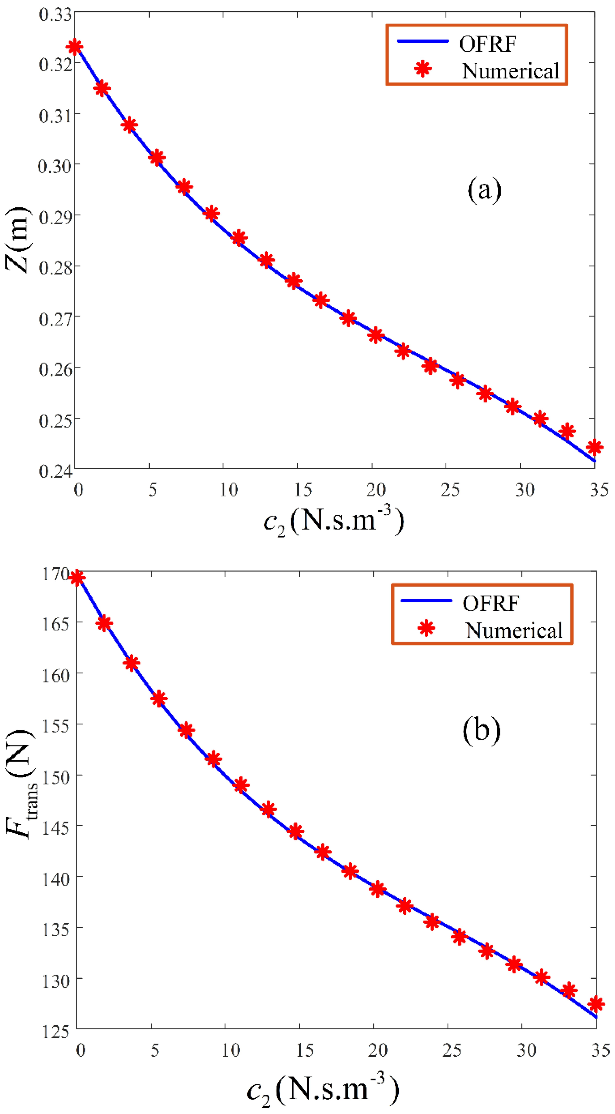
Figure 4.
Output spectrum of the transmitted force, .
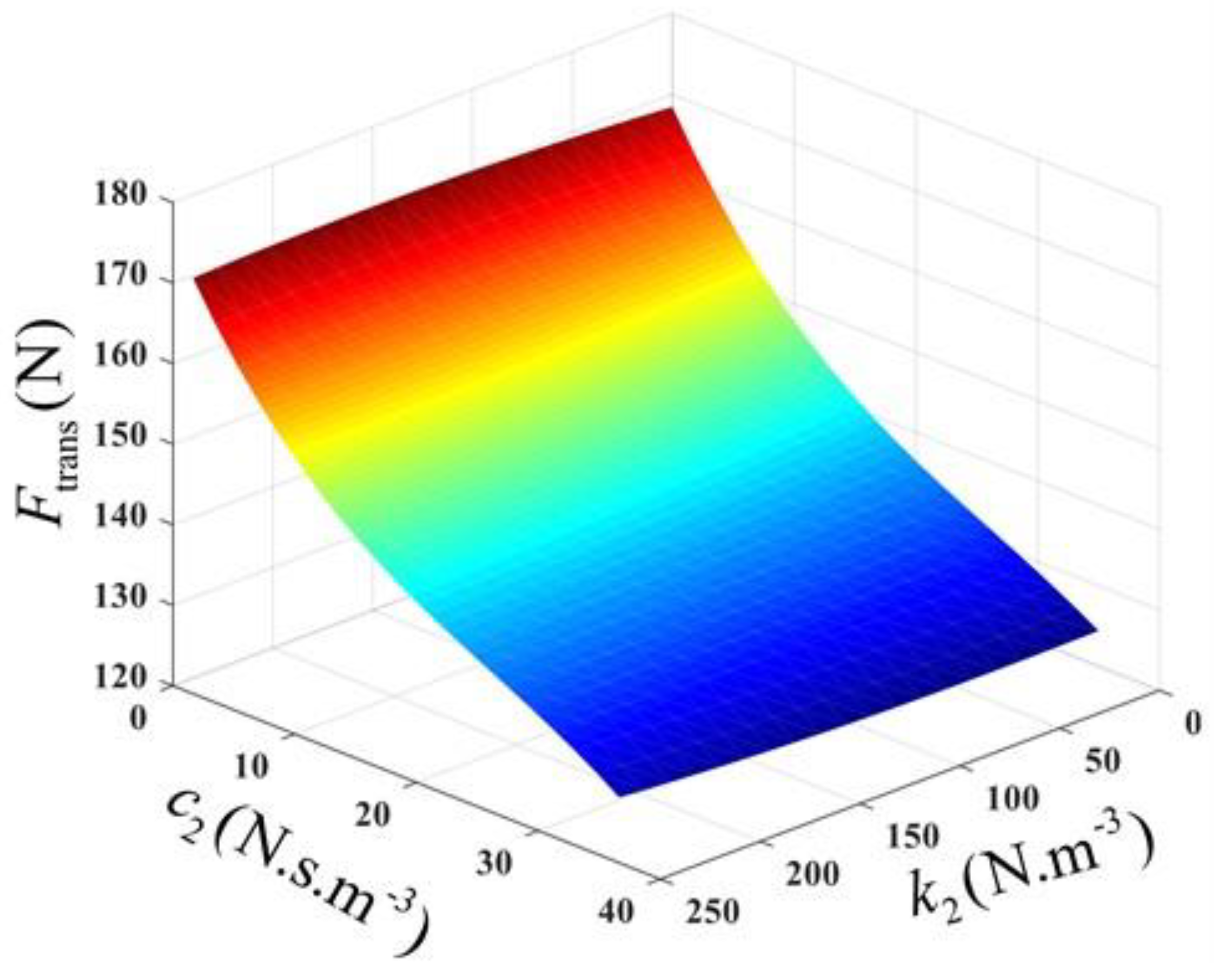
Figure 5.
Contour map of the Output spectrum of the transmitted force,.
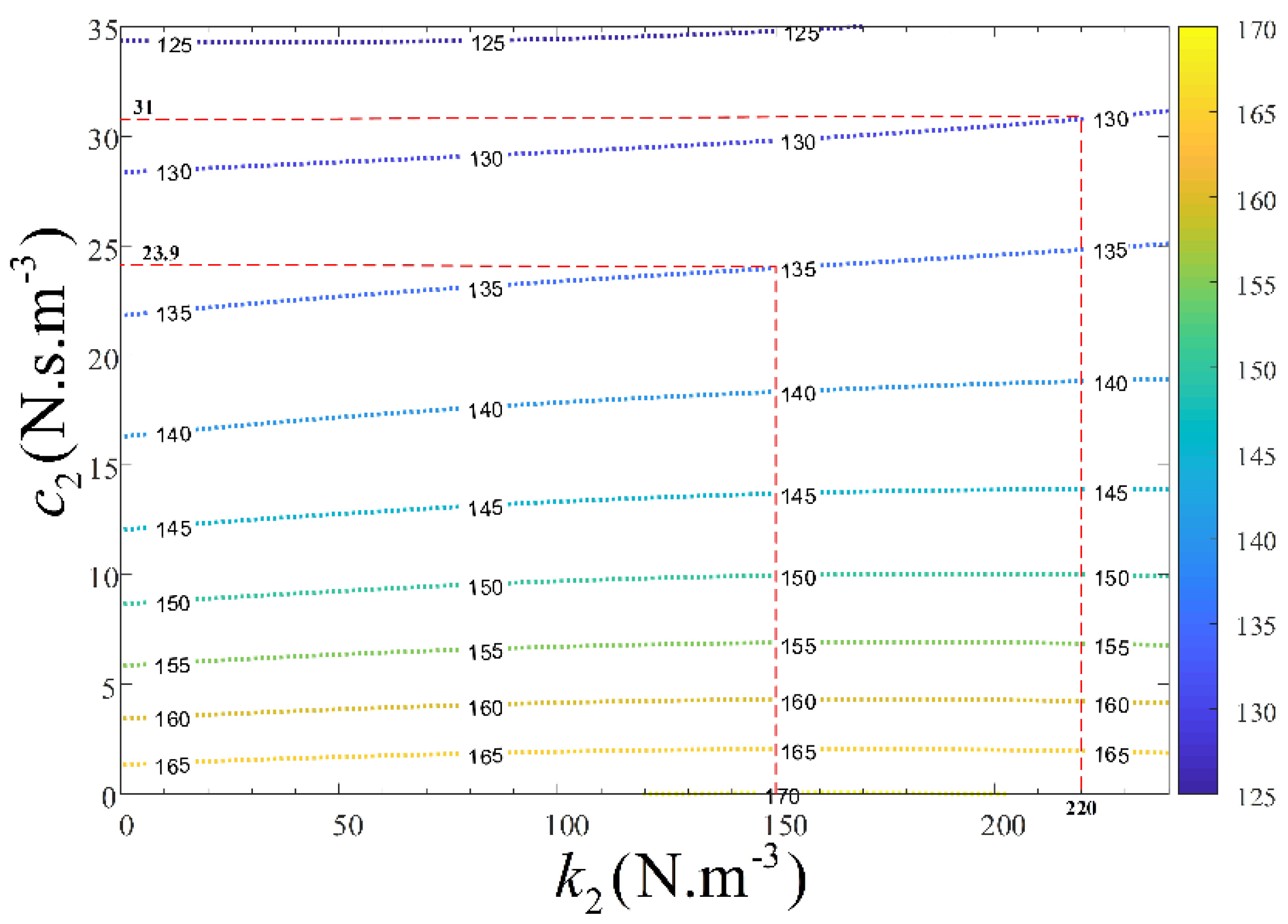
Figure 6.
Comparison of the system output response, at resonance, under linear and nonlinear conditions.
Figure 6.
Comparison of the system output response, at resonance, under linear and nonlinear conditions.
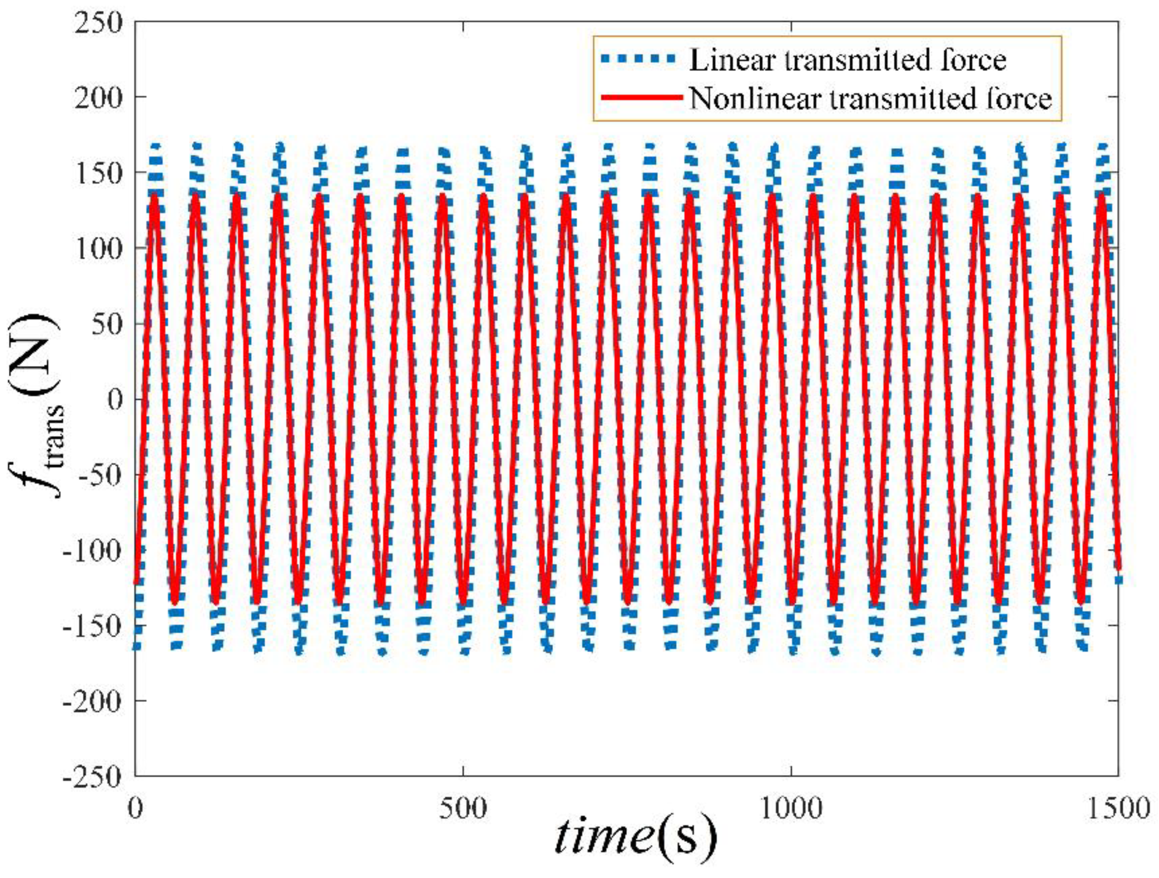
Figure 7.
Comparison of the system output spectrum, under linear and nonlinear conditions, across the entire frequency range.
Figure 7.
Comparison of the system output spectrum, under linear and nonlinear conditions, across the entire frequency range.
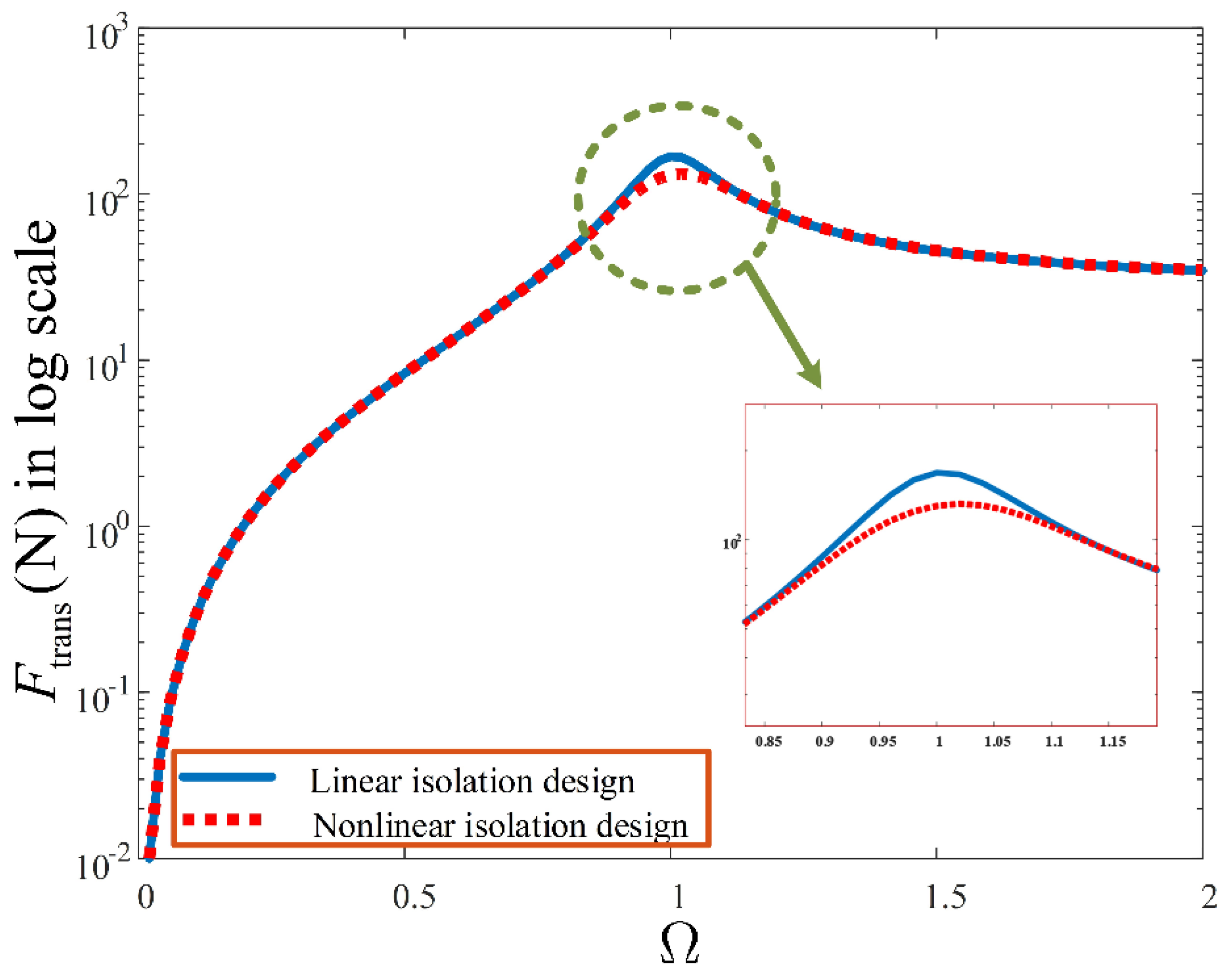
Figure 8.
Effect of linear damping characteristic parameter, on the system output spectra, across the entire frequency range, with N.s.m−3 and N.m−3.
Figure 8.
Effect of linear damping characteristic parameter, on the system output spectra, across the entire frequency range, with N.s.m−3 and N.m−3.
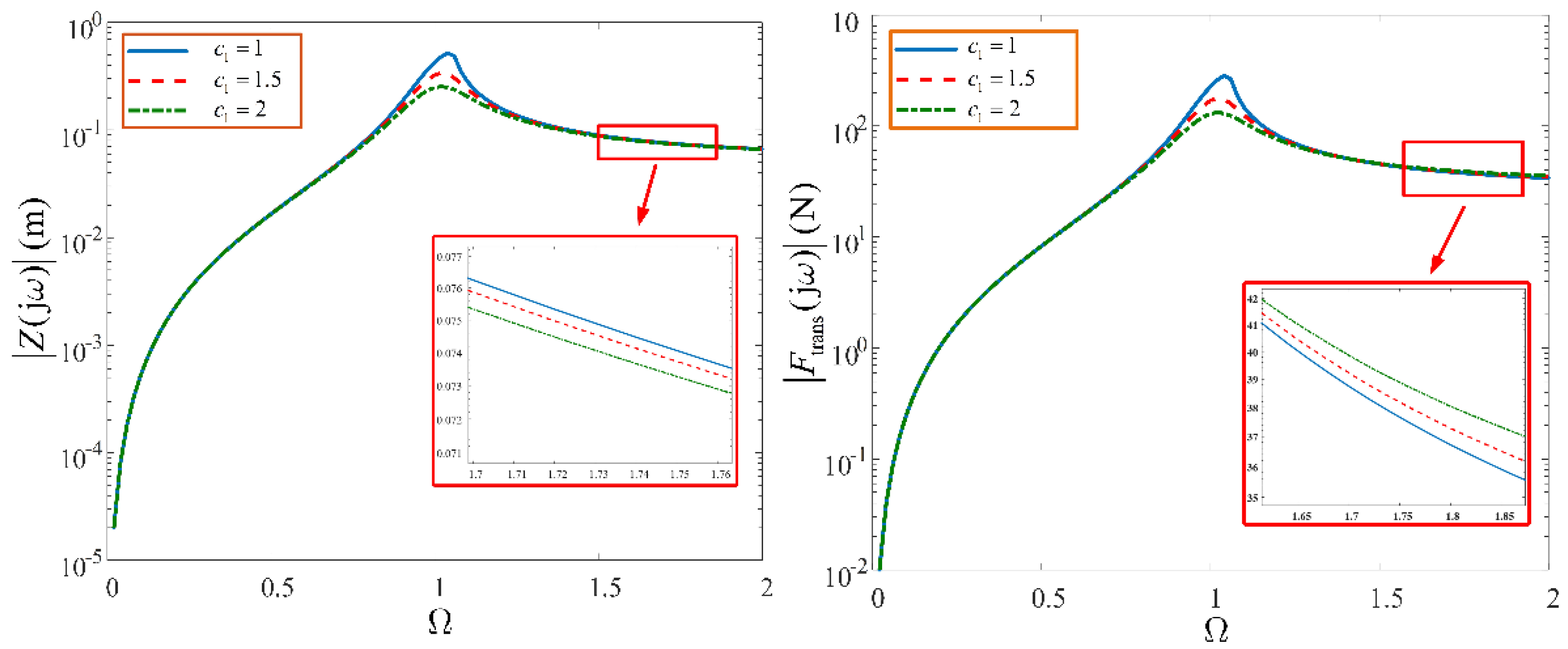
Figure 9.
Effect of nonlinear stiffness characteristic parameter, on the system output spectra, across the entire frequency range, with N.s.m−1 and N.s.m−3.
Figure 9.
Effect of nonlinear stiffness characteristic parameter, on the system output spectra, across the entire frequency range, with N.s.m−1 and N.s.m−3.
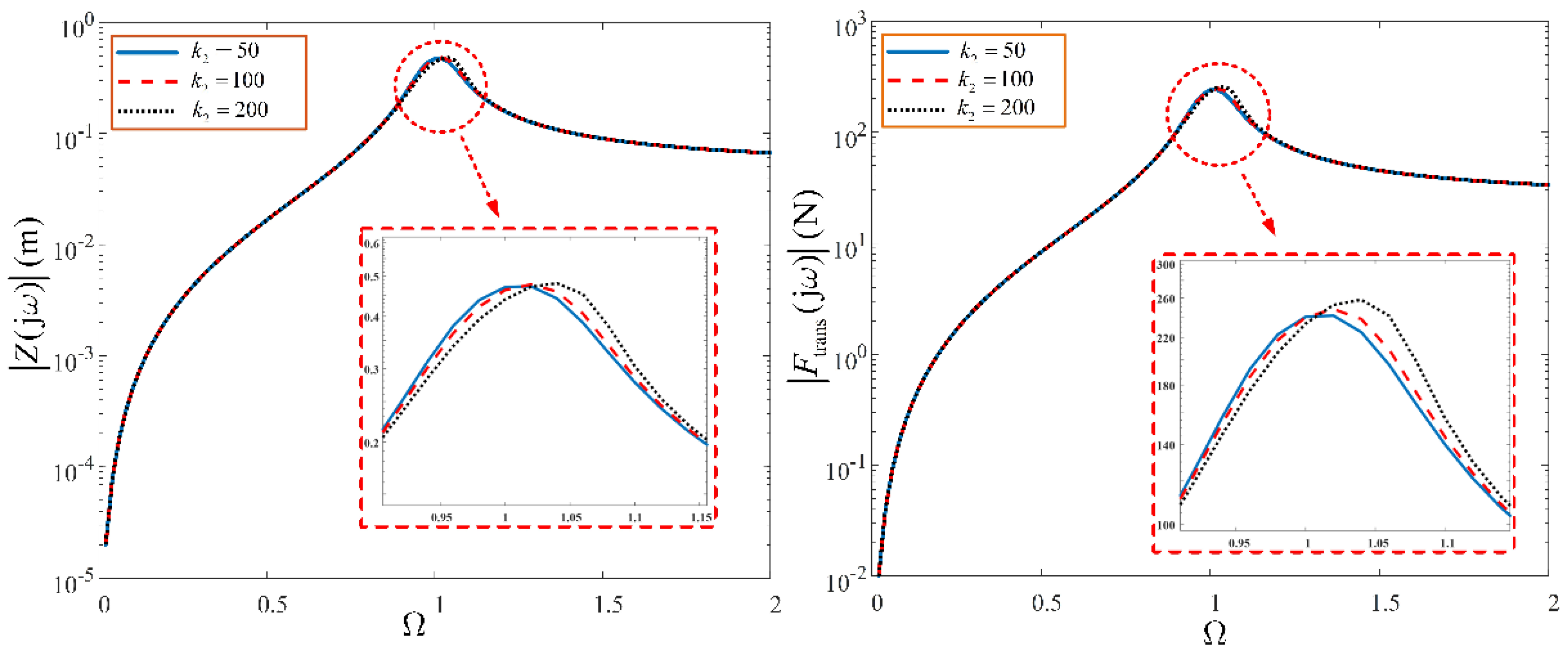
Figure 10.
Effect of nonlinear damping characteristic parameter, on the system output spectra, across the entire frequency range, with N.s.m−1 and N.m−3.
Figure 10.
Effect of nonlinear damping characteristic parameter, on the system output spectra, across the entire frequency range, with N.s.m−1 and N.m−3.
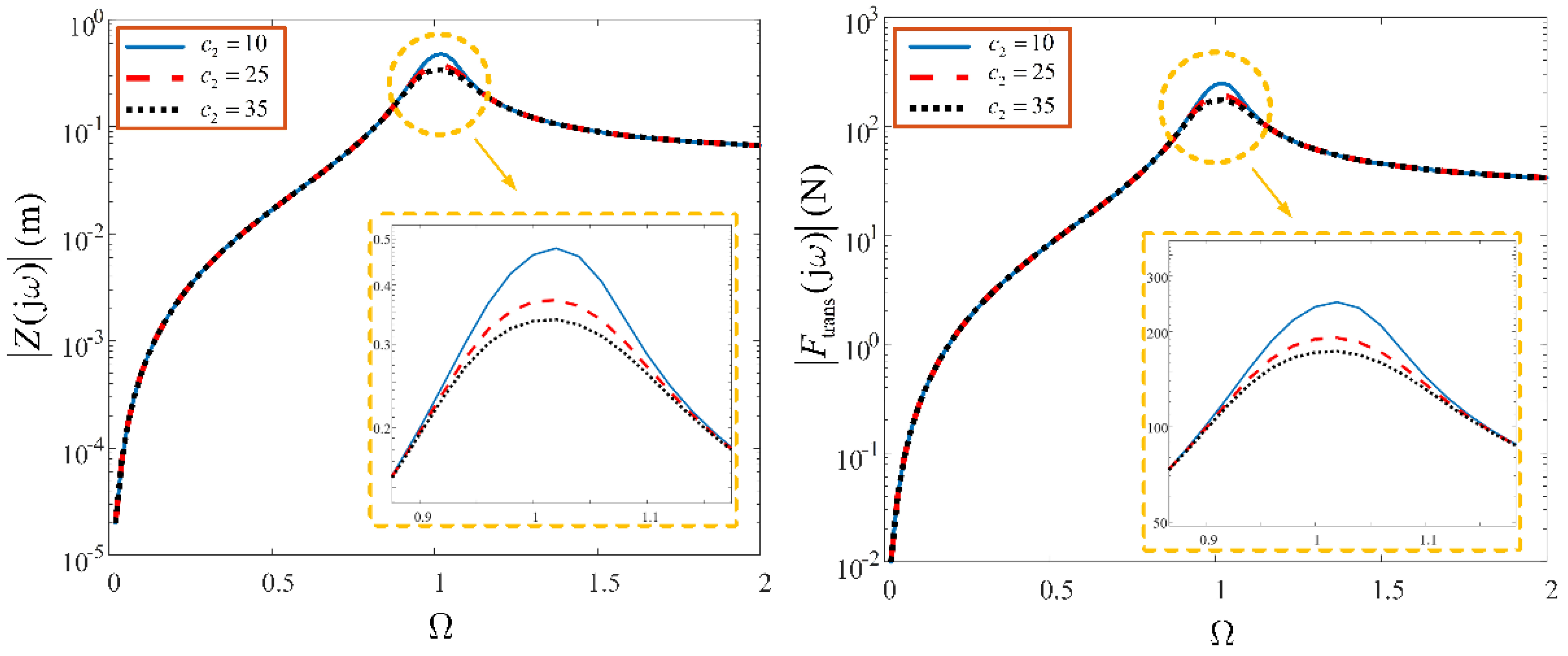
Figure 11.
Relationship between the Energy dissipation and design parameters, at .
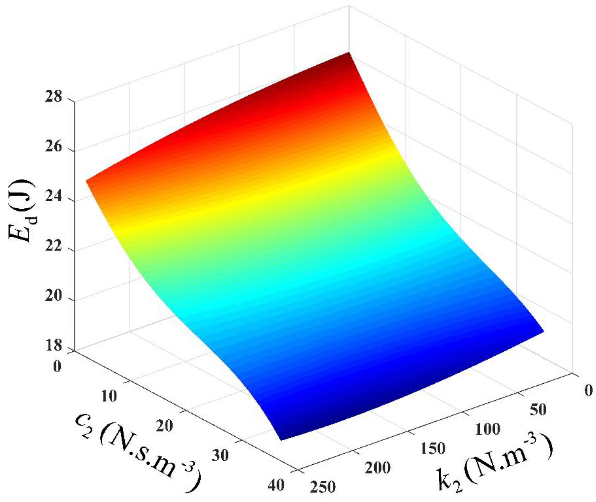
Figure 12.
Energy dissipation plot for sets of design parameters, at .
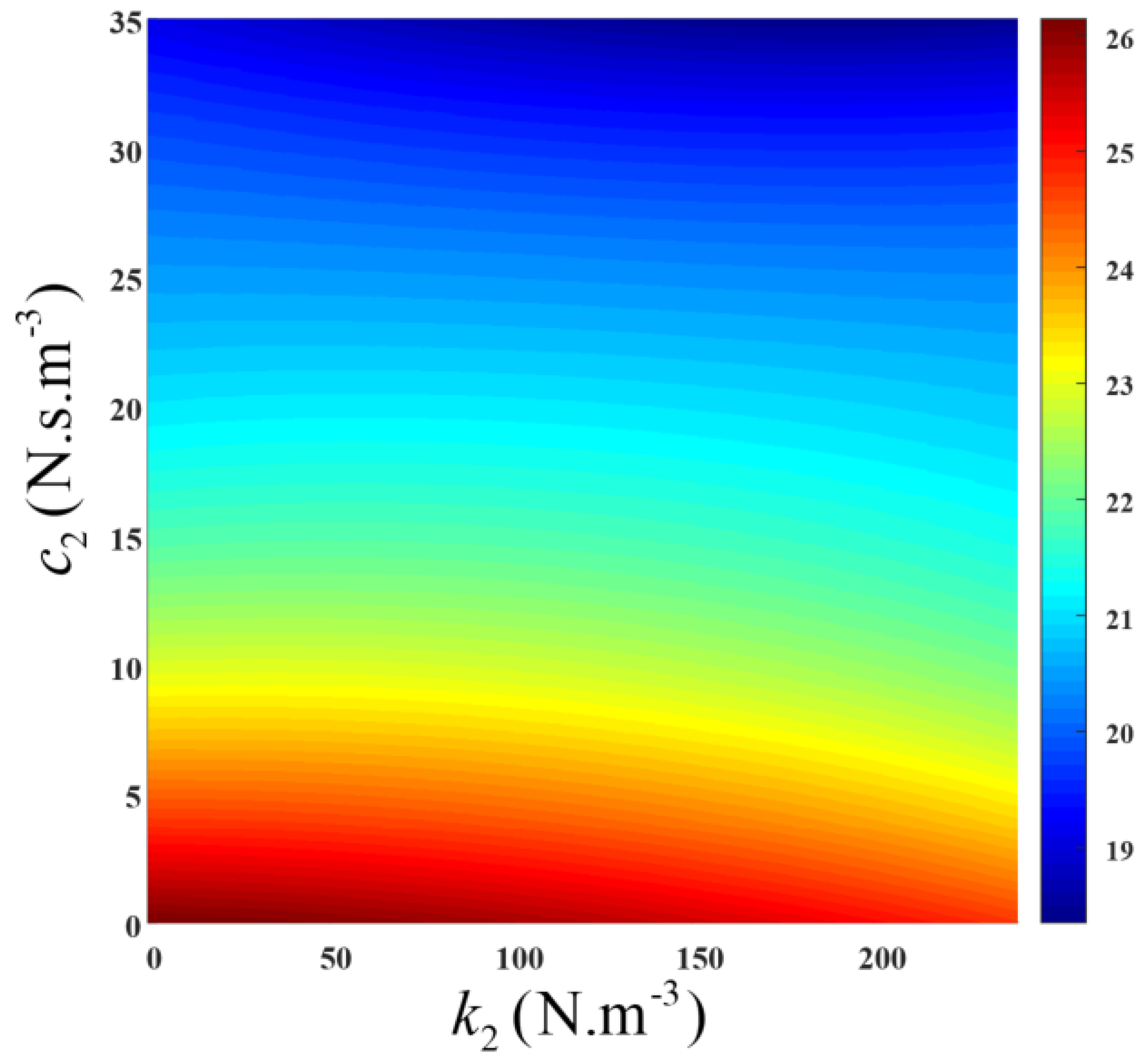
Figure 13.
Energy dissipation levels for different combinations of design parameters, at .

Figure 14.
Energy dissipation levels for different combinations of design parameters, at .
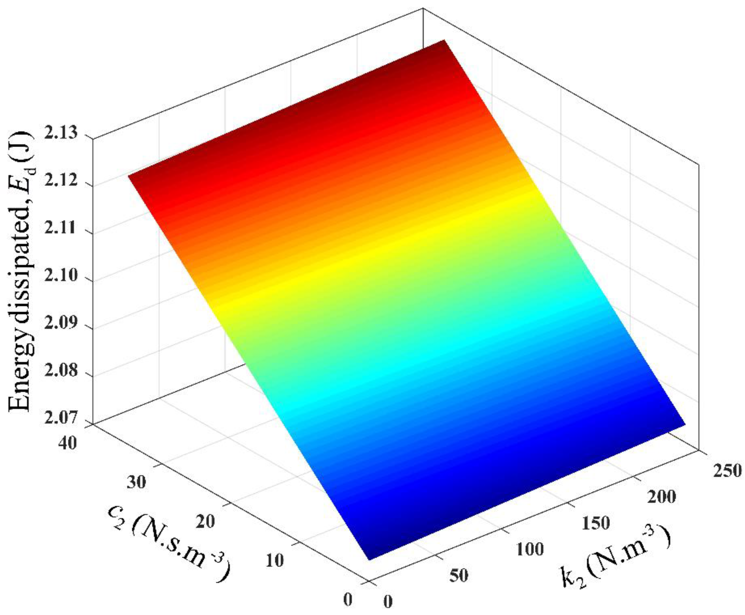
Figure 15.
Contours of energy dissipation levels, for sets of design parameters, at .
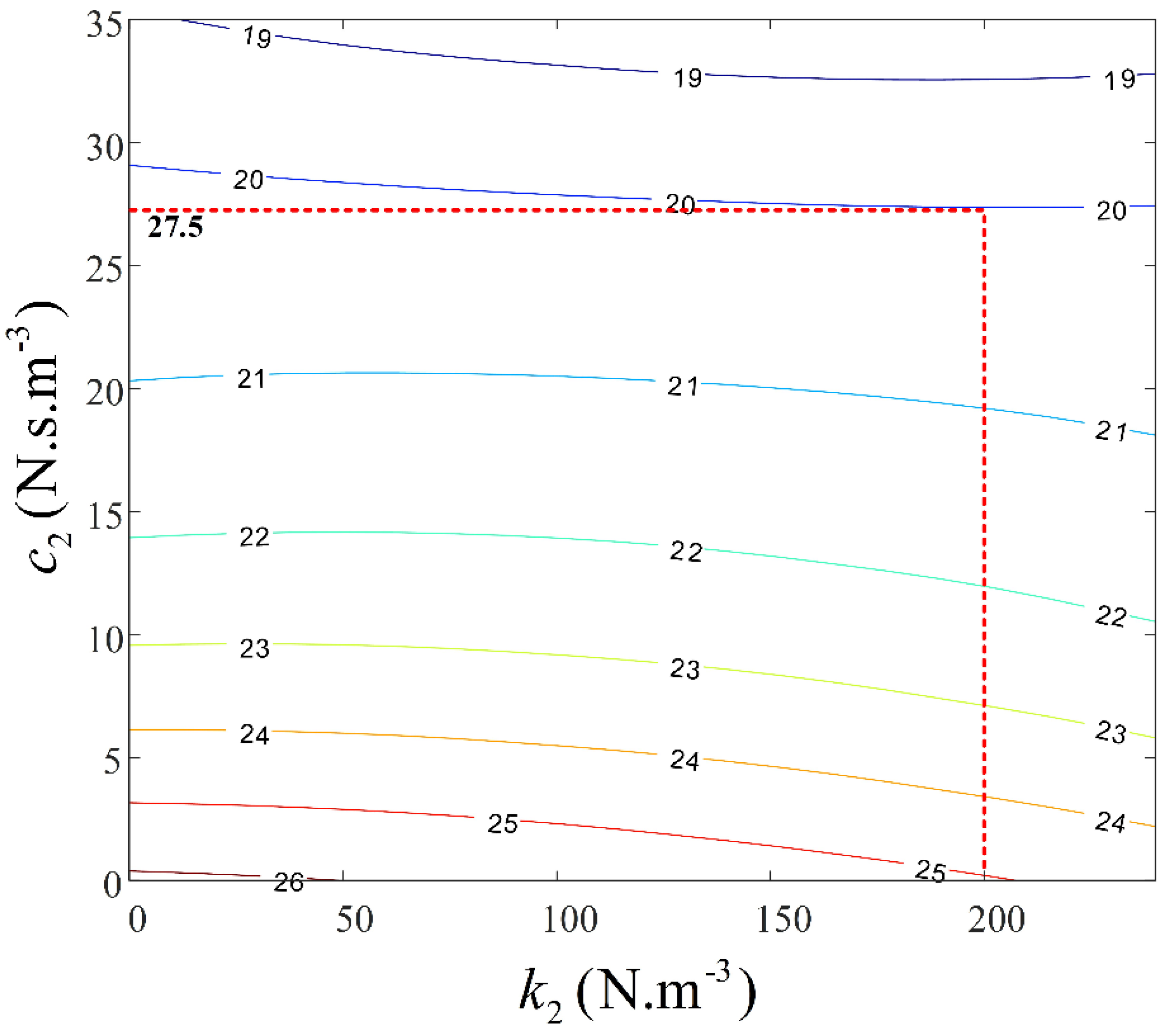
Figure 16.
Effect of the linear damping characteristic parameter, on the energy dissipation level, across all frequency range, with N.s.m−3 and N.m−3.
Figure 16.
Effect of the linear damping characteristic parameter, on the energy dissipation level, across all frequency range, with N.s.m−3 and N.m−3.

Figure 17.
Effect of the nonlinear damping characteristic parameter, on the energy dissipation level, across all frequency range, with N.s.m−1 and N.m−3.
Figure 17.
Effect of the nonlinear damping characteristic parameter, on the energy dissipation level, across all frequency range, with N.s.m−1 and N.m−3.
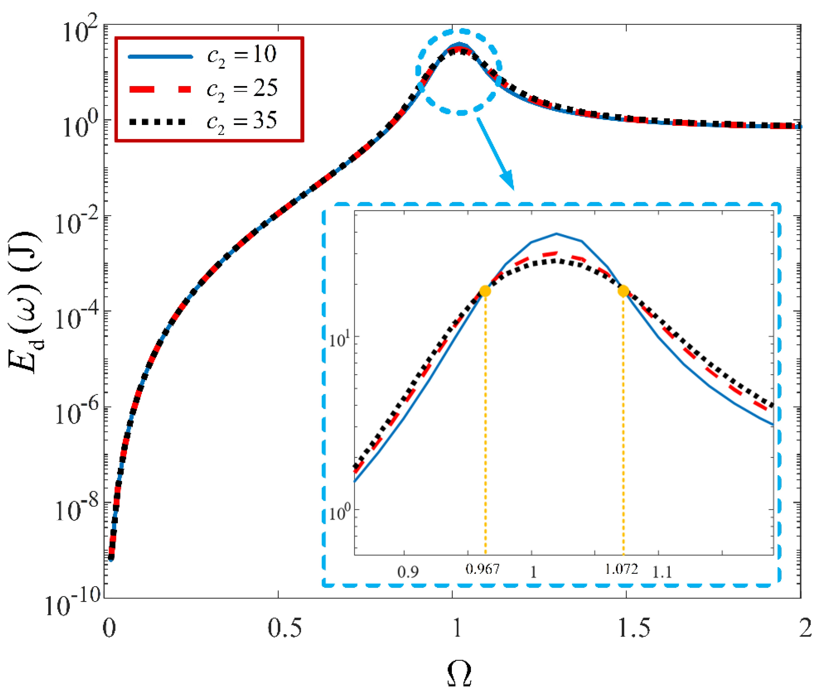
Figure 18.
Effect of the nonlinear stiffness characteristic parameter, on the energy dissipation level, across all frequency range, with N.s.m−1 and N.s.m−3.
Figure 18.
Effect of the nonlinear stiffness characteristic parameter, on the energy dissipation level, across all frequency range, with N.s.m−1 and N.s.m−3.

Figure 19.
Variation of energy dissipated and force transmitted by the suspension system, with respect to at N.s.m−1 and N.s.m−3.
Figure 19.
Variation of energy dissipated and force transmitted by the suspension system, with respect to at N.s.m−1 and N.s.m−3.
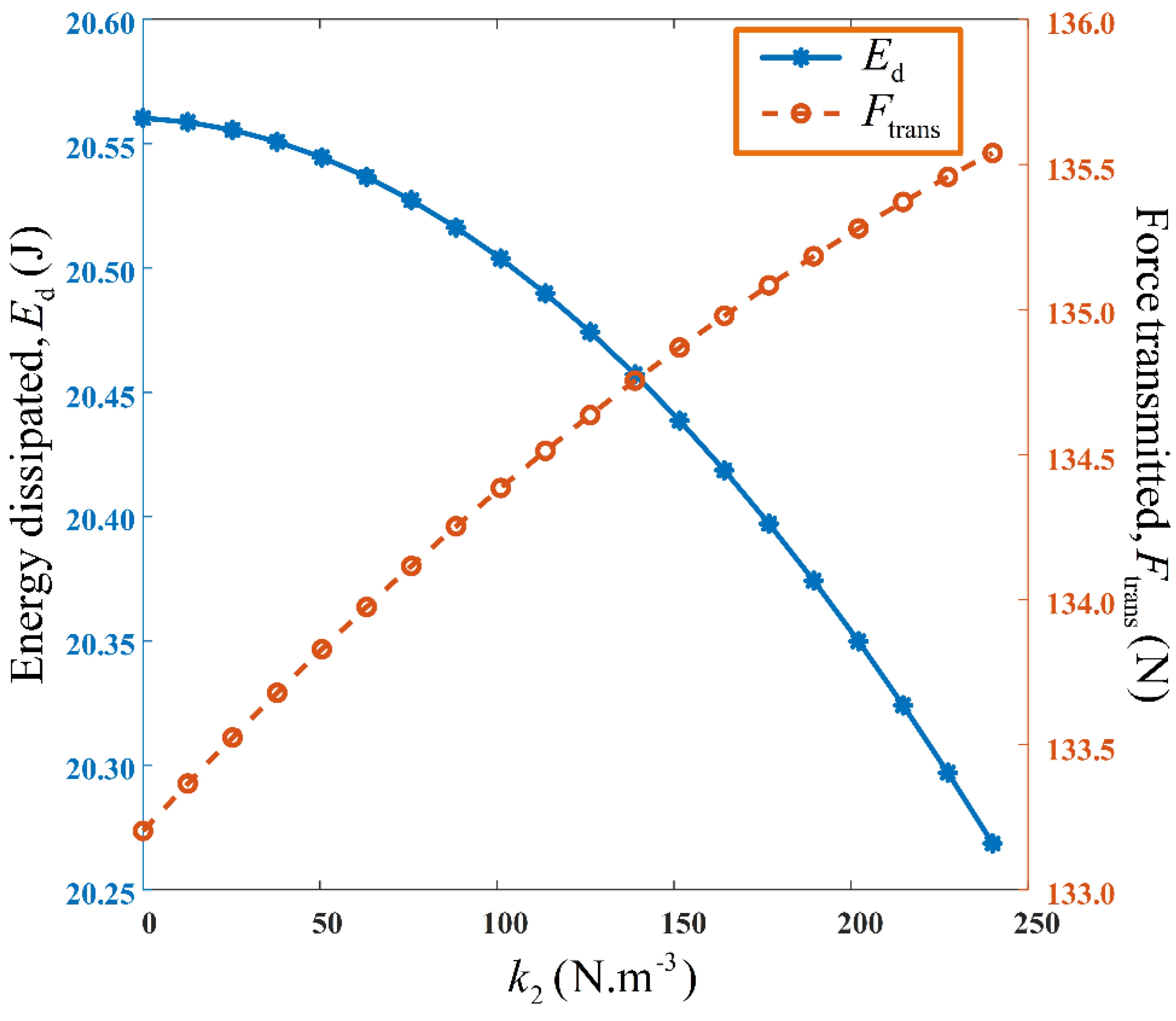
Figure 20.
Variation of energy dissipated and force transmitted by the suspension system, with respect to at N.s.m−1 and N.m−3.
Figure 20.
Variation of energy dissipated and force transmitted by the suspension system, with respect to at N.s.m−1 and N.m−3.
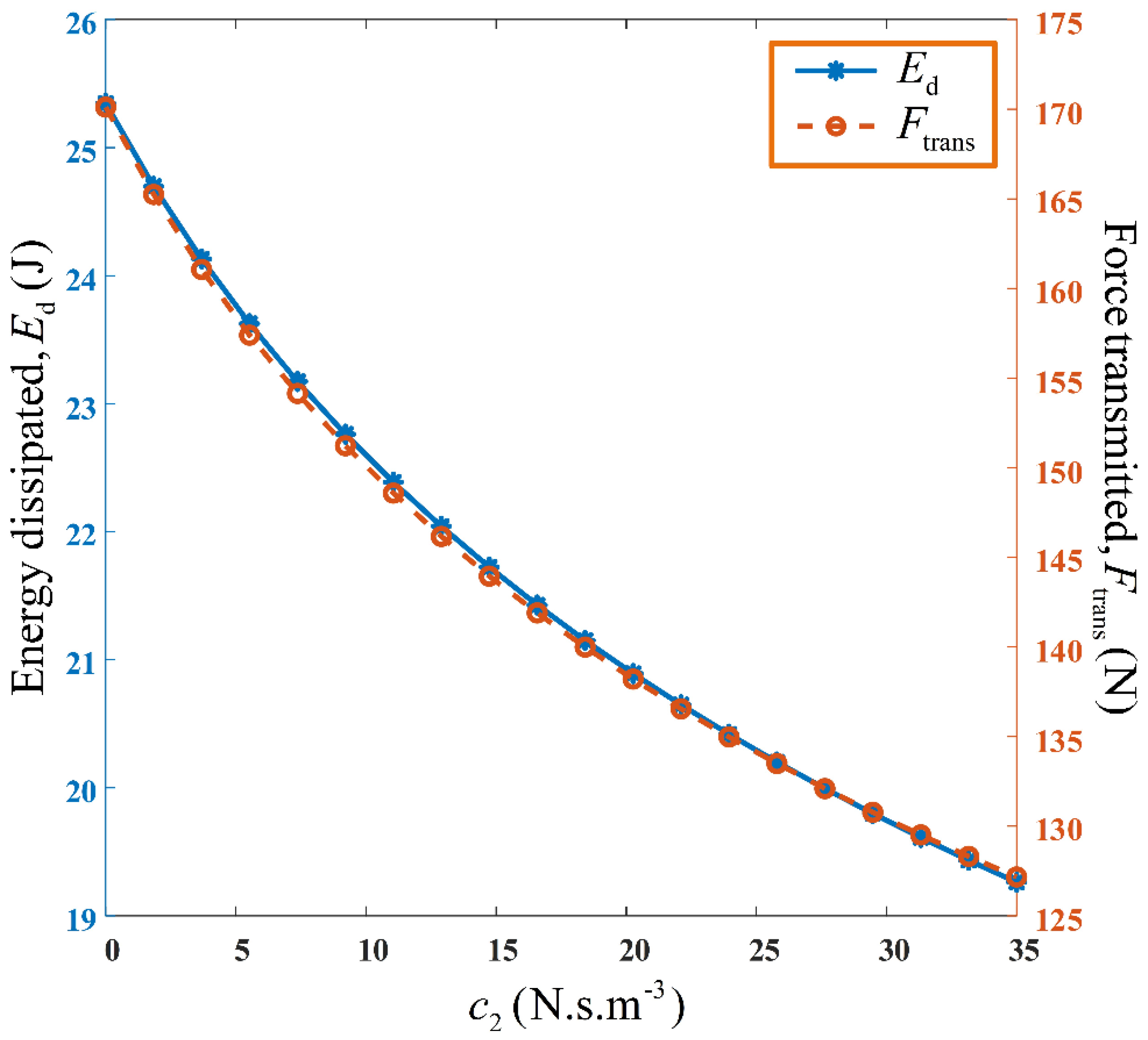
Figure 21.
Variation of the suspension damper force, and energy dissipated by the suspension system, with frequency at N.s.m−1 and N.s.m−3.
Figure 21.
Variation of the suspension damper force, and energy dissipated by the suspension system, with frequency at N.s.m−1 and N.s.m−3.
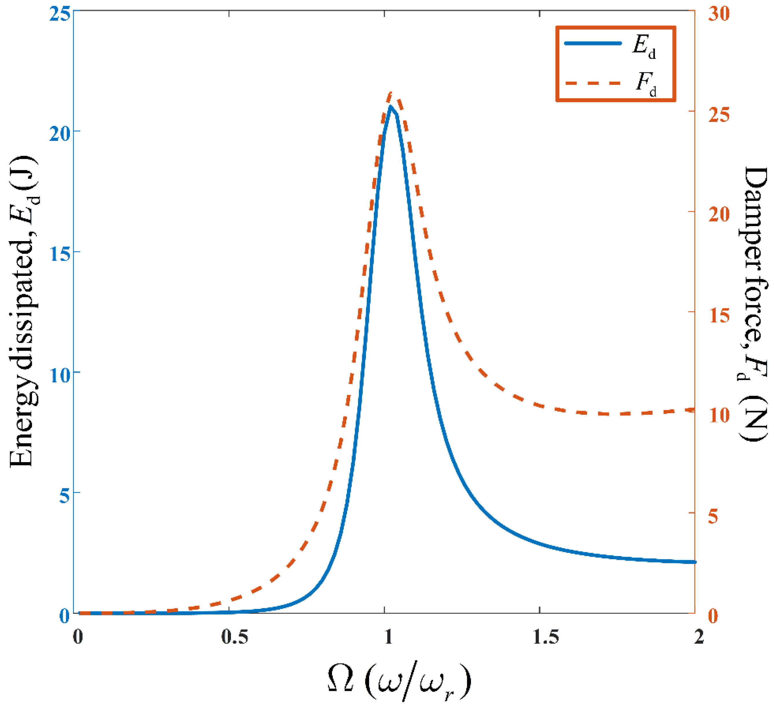
Figure 22.
Comparison of the Hysteretic curves for the vibration isolation system, having different combinations of nonlinear parameters, at resonance. (b) is shown in Figure 23.
Figure 22.
Comparison of the Hysteretic curves for the vibration isolation system, having different combinations of nonlinear parameters, at resonance. (b) is shown in Figure 23.
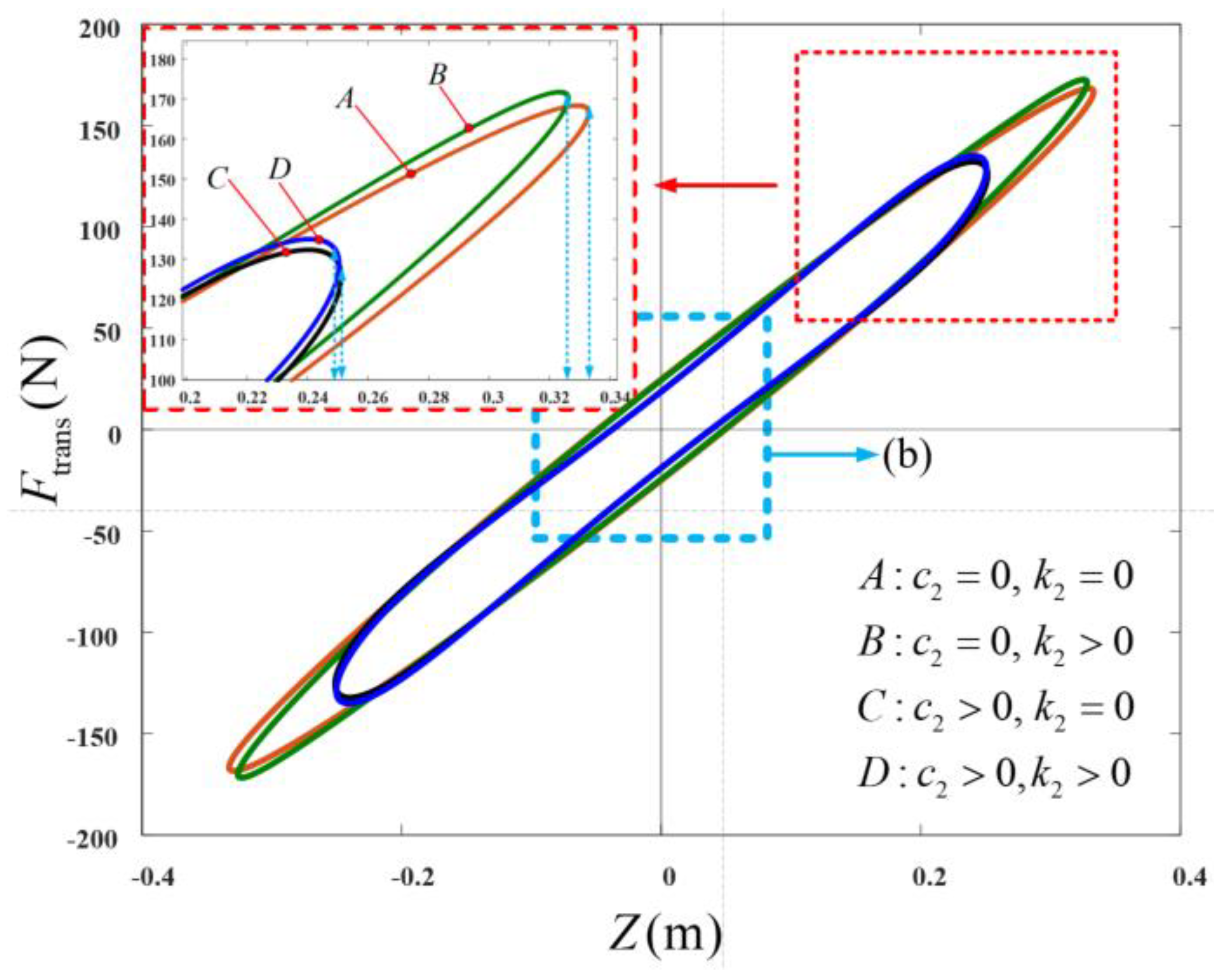
Figure 23.
Enlarged origin of the hysteresis curves in Figure 22.
Figure 23.
Enlarged origin of the hysteresis curves in Figure 22.
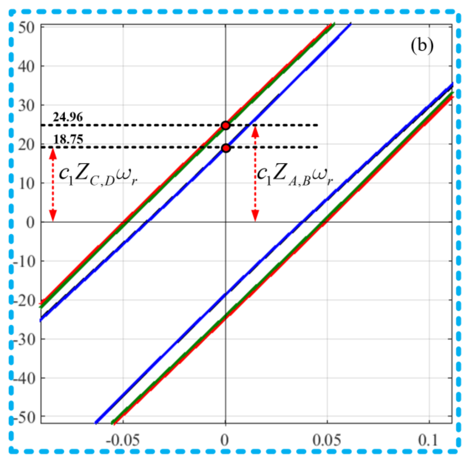

Table 1.
System parameters.
| Parameter | Value | Unit |
|---|---|---|
| 0.2 | kg | |
| 1.5 | N.s.m−1 | |
| 0.05 | m |
Table 2.
Results from the optimisation problem.
|
Desired output response, |
Actual output response |
|||
|---|---|---|---|---|
| 135 | 150 | 23.9 | 134.8924 | 7.9767 × 10⁻² |
| 130 | 220 | 31 | 130.1583 | -1.2162 × 10⁻¹ |
Disclaimer/Publisher’s Note: The statements, opinions and data contained in all publications are solely those of the individual author(s) and contributor(s) and not of MDPI and/or the editor(s). MDPI and/or the editor(s) disclaim responsibility for any injury to people or property resulting from any ideas, methods, instructions or products referred to in the content. |
© 2024 by the authors. Licensee MDPI, Basel, Switzerland. This article is an open access article distributed under the terms and conditions of the Creative Commons Attribution (CC BY) license (http://creativecommons.org/licenses/by/4.0/).
Copyright: This open access article is published under a Creative Commons CC BY 4.0 license, which permit the free download, distribution, and reuse, provided that the author and preprint are cited in any reuse.


