Submitted:
02 August 2024
Posted:
06 August 2024
You are already at the latest version
Abstract
Balandra, one of the most popular beaches in La Paz, Baja California Sur, was declared a flora and fauna protection area in 2012 and, in 2021, was declared the best beach in Mexico. More recently, it was included among the ten most beautiful beaches in the world. Currently, this beach faces overcrowding. Formulating effective management policies depends, to a certain extent, on the knowledge of their recreational value and visitor characteristics. Recreational value allows us to know the benefits of the tradeoffs among the ecosystem services and society and exhibit the value of possible damages to marine ecosystems. Like the one caused in 2022 by the fire of a tourist boat inside Balandra. Using the individual travel cost method and applying 159 questionnaires to site visitors, four models were estimated to calculate the individual willingness to pay for accessing Balandra, which ranges between 3.86 and 10.38 US$/day/visitor. Recreational economic value (REV) for Balandra was estimated using two essential criteria. One, total of visitors registered in 2021. Two, daily maximum carrying capacity. We also calculated the REV as a proxy of the welfare loss derived from the site's closure. Finally, possible environmental and economic policy instruments that could be implemented are discussed.
Keywords:
coastal tourism
; marine protected area
; Gulf of California
; count models
; truncated Poisson
; negative binomial model
1. Introduction
Marine protected areas (MPAs) are a recurrent mechanism to safeguard marine ecosystems and biodiversity [1]. MPAs provided benefits derived from their conservation, such as recreational benefits provided to beach swimmers in coastal zones. To ensure that these benefits are considered and endured, MPA management requires continuous surveillance and monitoring. These latter are not free, and because of that, managers set access fees. In several countries, the coastal and beach tourism industry is a source of significant economic benefits.
Natural diversity contributes to a massive demand for touristic services, mainly in MPAs, since using mega-diversity for recreational purposes has generated significant income levels in coastal communities. Nevertheless, there has been an accelerated increase in tourism and the demand for ecosystem services in coastal communities, even small ones, which depend on tourism as a primary or complementary means of livelihood [2].
These zones are highly linked to marine resources and attractions, such as crystal waters and environments suitable for practicing touristic sports and activities. Because of this, coastal zones are relatively relevant due to their social, ecological, cultural, and economic value. Emerging economies seek to exploit their tourism potential to catapult economic development without affecting them [3].
Coastal and marine environments attract hundreds of millions of tourists annually; tourism is a pillar of local economies in some regions [4]. Nature tourism contributes almost 7% of world tourism expenditure, and wildlife tourism contributes 343 billion US$ globally [5]. Many tourism activities focus on “Sun & Sea,” based on marine resources. Tourism depends on the integrity of coastal resources, i.e., beaches and water. Despite the economic importance of tourism, coastal resources have become scarcer and threatened by it. Several beach destinations have taken measures to deal with them, like long seashore structures or dredging. Such measures regularly bring non-accepted consequences, locally or elsewhere [6]. External pressures on coastal zones linked to tourism, such as land transformation and construction of industrial developments, water pollution, mangroves depletion, invasive species introduction, and exhaustive use of resources (for example, marine species used as meals and souvenirs), plus climate change; affects tourism viability and tourism coastal destinations [4]
The need to keep attractive beaches for tourists has frequently led local managers to clean these [7]. A good perception and attitude to the recreational site is essential for tourist demand [8,9,10]. However, such cleaning actions usually generate environmental externalities or damages in coastal ecosystems, like coastal line disruption, marine and coastal biodiversity reduction, and marine and coastal waste disposal (mainly algae, birds, and dead biota) [11]. However, beach cleaning is often needed to maintain tourism affluence and activity [12,13,14]. Nevertheless, environmental issues could be accumulative.
Tourism also generates social externalities, such as access loss to public or beach facilities, pollution, beach crowding, infrastructure construction, and artificial covers in sandy beaches, dunes and mangroves, waterfront and coastal line modifications, loss of cultural and religious values [15]. In these two situations, coastal ecosystem management prevails; a wide gradient of management instruments/tools is available, which could help management be more efficient considering the associated costs [16]. These tools must seek to minimize or eliminate externalities. MPAs’ popularity is increasing, but management and conservation strategies to secure a sustainable anthropogenic use inside them are still under debate [15,16].
Externalities could be minimized by applying environmental valuation (EV) and its specific techniques [17,18]. Among them are the stated preference methods (contingent valuation) and the revealed preference methods (travel cost and hedonic prices). EV contribute to the design of economic instruments for environmental policy (EIEP), which are oriented to modified consumption or production patterns and strengthen environmental planning instruments or compensatory (or regulatory) instruments for conservation [19]. EIEP could also contribute to MPA’s sustainable financing by using market mechanisms as compensatory instruments, voluntary markets, shared schemes, concessions, payments for environmental services, revenues, fees, charges, and commercial operations of MPAs [20].
Economic research contributes to the debate on MPAs as a management option assessing the cost and benefits for society (Table 1). This research could show how coastal zone value is modified, including beaches, with or without MPAs. Some costs are often accessible to estimate; however, some benefits, like recreational, conservation (future use), and ecosystem functions, are rarely incorporated [7].
1.1. Balandra Flora and Fauna Protection Area
Baja California Sur (BCS) is positioned as Mexico’s fifth tourism destination and the third destination that received the most tourists by air and sea [28]. BCS’s central natural heritage is constituted by high biodiversity (ecosystems and species), landscapes, and beaches, on which it is possible to perform different social and economic recreational activities [2]. La Paz’s beaches stand out for their low slope and soft white sand; beaches like Balandra, El Tesoro, Coromuel, El Caimancito, and Pichilingue are some of the favorite beach destinations of national and international tourists [29]. Balandra became a natural protected area due to its high marine and terrestrial biodiversity.
Balandra was declared a natural protected area (BNPA) in 2012 [30]. It is located east of La Paz Bay (Figure 1) and incorporates the largest wetland in the bay of La Paz, Balandra and El Merito wetlands refuge of species of red, white, and black mangrove; it houses 13 species of macroalgae (seagrasses), 56 fish species and 30 of birds, fin whale, humpback whales, orcas and dolphins have been sighted. San Rafaelito protects a colony of California seals. The area of seagrasses and mangroves functions as a nursery habitat for fish and invertebrates of commercial interest. It highlights eight bays with white beaches and a mushroom-shaped rock formation [31].
Tourism is the main activity in BNPA, but there are also small-scale and recreational fisheries [30,31]. Tourism has increased since the federal government declared it the best beach in Mexico [32,33]. Because of its unique and barely unmodified landscapes and clean beaches, it is one of the most visited beaches in BCS [34].
A sudden tourism demand increase has generated some issues in BNPA; one, a severe over-crowding; BNPA carrying capacity (CC) is 350 persons/day in the main beach (Balandra A), and the full CC for the area is 984 persons/day [44]. Due to overcrowding, current visitor management strategies consist of two daily visiting shifts, with a maximum of 400 people on Balandra’s main beach [35,36,37]. This strategy tries to accomplish 800 visitors/day in BNPA main beach, exceeding its CC by 2.28 times.
On August 21st, 2022, BNPA faced a maritime accident inside the marine zone; a tourist boat caught fire when passing by this zone, which is restricted to naval navigation. Carrying out marine and coastal pollution by the fuel and oil spill in the influence area where it took place, besides the boat physically burned waste was left on the beaches. Because of this accident, BNPA remained closed for over two months that year [38,39].
These issues lead to two questions: Can overcrowding be controlled by setting higher access fees? Two, what is the economic impact on on-site recreation from the damage caused by the maritime accident in the area? To answer these questions, we proposed using the individual travel cost method.
2. Materials and Methods
3.1. Sampling
Managers from BNPA reported 41 259 visitors in the 2020-2021 season. Applying proportional unrestricted random sampling for each month of the season, the sample for this research was estimated using parameter values as p=0.5, q=0.5, an estimation error (i) of 7.7% and 95% confidence; we obtained 161 questionaries to be applied face to face to visitors from April 2021 to March 2022. The response rate was 88%.
3.2. Questionnaire
Due to COVID-19 pandemic restrictions, we used a Google Forms online questionnaire. The questionnaire is divided into three sections. The first is “Travel,” where visitors are asked about the visit motivation, transportation means, travel, and discretional costs (2021 US$). The second, “Site,” includes questions about visits to BNPA and the site’s environmental conditions. Third, “Visitor characteristics,” like precedence, distance, and socioeconomic and sociodemographic aspects.
3.3. Travel Cost Method
From an economic perspective, recreational services provided by natural resources (lakes, rivers, estuaries, beaches, forests, and others) have essential attributes and characteristics. These latter are fundamental to determining the economic value of recreational services. The market system does not assign access to natural resources that offer recreational alternatives. This means that natural resources providing recreational services are public goods. A prevalent methodology to assign their economic value is the travel cost method (TC). The method was proposed to the National Park Service of the United States of North America to establish access fees [40]. During the 1980’s decade, TC applied two approaches to recreational studies: individual and zones. A decade later, when microdata was available, conjointly with a better understanding of the aggregation biases of the method, ITC was chosen over the zone method [41].
The method foundations are that a visitor must incur travel and other costs associated with visiting one specific site to enjoy its recreational services. It seeks to estimate how the demand for environmental assets varies, considering how the number of visits will change if there are also changes in the travel cost. TC has seven basic assumptions: i) trips and environmental quality of the site are complementary in the demand function, ii) individuals perceive and respond to travel cost variations in the same way that they will respond to changes in site access fees, iii) single site visit, iv) individuals do not perceive utility or disutility during the trip or during his working time [42].
TC has some issues to consider, among them are: i) the equipment maintenance costs could be high or low, depending on its specialization or season, ii) incorporation of cost for multi-site or multi-purpose travels lacks theoretical bases, iii) lodging and feeding costs have a high discretional component, should all these costs must be accounted for? iv) including substitute sites and/or activities influence on welfare estimation; besides, there is not conceptually straightforward if these substitutes must be considered, v) recreational preferences could influence traveled cost or distance, or could be considered as an exogenous variable and, vi) there is no theoretical and clear consensus about how to include the opportunity cost [43].
A general outline of TC assumes a tourist visiting a single recreational site has a determined budget and an unrevealed value with which they compare actual prices before making the visiting decision. Considering the different preferences and income levels, this allocated budget is distributed among individuals through the travel cost for visiting the site; there will be individuals whose willingness to pay (WTP) for accessing the site is high, and others whose WTP to access the site is lower. This condition originates a demand curve, which relates the different costs and expenses of traveling to the site with the number of visits an individual makes [42]. Individual travel decisions related to cost differences are modeled from choosing a certain number of trips for a certain period. Finally, the value of a particular site’s recreational service flow is represented by the area under the compensated demand curve, aggregating all site visitors [44].
ITC is characterized by its benefits in estimation efficiency for the demand function for recreational services. The general ITC outline is.
Where Xij is the individual number of visits to the recreational site in one year, Cij is the personal travel cost, Zij is a vector of socioeconomic and environmental variables related to the individual and the site, and εij is the stochastic term.
Xij=f(Cij,Zij,εij)
3.4. Poisson Models for Recreation Demand
Individuals frequently make just a few numbers of visits to a recreational site, with one or two trips as the maximum. Most ITC models are estimated using discrete distributions. Since the number of trips is a non-negative discrete variable, it is the dependent variable. Under this approach, discrete density functions such as the Poisson distribution have been decided to be used. The most relevant feature of Poisson models is that they assume equality between the distribution’s mean and variance [42,45].
Recreational demand could be estimated using ITC; the method shows the individual’s willingness to accept or behave in favor of site improvements or how the individual values potential site damage. If such changes happen, such willingness is measured through the number of trips and the associated costs to access the recreational site (and other socioenvironmental variables) [45].
The individual demand model allocates time and income constraints, providing a generic demand function for a single site. Assuming that an individual, i chose xij; where j is the number of trips/visits to the site ∀ j=1, 2,…n. Round TC is cij. The individual also consumes a set of associated goods zi, also known as weak complementarity goods. TC assumes that the visitor is subject to two constraints [46]:
Where tij is the travel time to the site, j; h is associated with the individual working hours, and T is the individual total available time. It also assumes that visiting time for every site is the same.
With explicit arguments individual demand i for site j, is given by ), where is the individual full income (; or the amount of money the person could earn if he worked his whole available time, wi, is income after paying taxes, each qi is the exogenous quality of the jth site, and is the individual adjusted income by ; where is the individual income.
Once the general demand model has been defined, estimating the associated parameters for each trip determinant is possible. The most common model in TC is the Poisson count model. The Demand curve is determined for each individual site i in a given population is given as ; where and, . Poisson models specify the demanded quantity, trips, as an integer nonnegative random number, with mean independent from exogenous regressors. The expected functional form for Poisson models is typically exponential. For single site models, as this, the general count model is written as and the probability density function is ; where and is specified as an exponential function .
However, if the assumption of equality between the Poisson model’s mean and variance is empirically invalid or if data are generated by a mechanism that structurally excludes zero counts, the regressor will probably be biased. In this case, truncated count models are recommended.
3.4.1. Truncated Models
Truncated count models must be used if at least one of the following three situations exists. One, data came from a mechanism that structurally excludes zero counts, as in this case (Figure 2); under this assumption, Poisson distribution must adjust only when data values begin at one [48,49]. Two, if on-site sampling is conducted, it ensures that questionnaires are applied to visitors. The on-site sampling allows only visitors with trips xi>0 to be interviewed. In the on-site interviewing process, there is a high probability of interviewing visitors with a high frequency of site visitation since these individuals are more likely to be selected, known as truncated error or truncated demands [45]. Third, if a population that visits a recreational site is considered and divided into strata based on the number of trips, such that the stratum i, contains individuals who make i trip, it causes endogenous stratification.
This phenomenon occurs when the systematic variation in the selected proportion depends on the characteristics of the individuals in the sample or when the proportion of individuals chosen systematically varies from the population proportion. For distributions presenting these issues, the truncated Poisson model and the model with endogenous stratification can be applied [49,50].
3.4.2. Negative Binomial Models
The estimator for the truncated model could be biased and inconsistent under the presence of over-dispersion (α), defined as the excess of conditional variance over the corresponding conditional mean of the dependent variable (when the ratio variance-mean is higher than one). In such conditions, the negative binomial distribution must be used as an extension of the Poisson distribution [45].
For the negative binomial distribution, the functional form of λ is with a gamma distribution with mean of 1 and variance α. Besides, the random independent variable is λ and its variance . The ratio mean-variance is , such as the over-dispersion degree is a function related to λ and α. If , implies no data over-dispersion, and the negative binomial distribution is reduced to a Poisson distribution on its limit. However, when using negative binomial models, if the on-site sampling problem exists, if a mechanism that structurally excludes zero counts was used to collect data, or if there is a presence of stratified bias, it is highly recommended to use negative binomial truncated models [47,48].
3. Results
3.1. Descriptive
For continuous variables, the sample behaves as follows: an average of 6.81 visits to BNPA in the last five years, 12 days of staying, and five persons traveling with the interviewee. For monetary variables, averages are in US$ 652 for monthly income, 44 for travel cost to BNPA, 65 for daily feeding expenses, 125 for daily lodging rate, and a total cost of 230. Frequencies for categorical variables are 62% male and 38% female; visitors are disaggregated as follows: 24% domestic, 27% American (USA), 21 Europe, and 28% another precedence. 42% of domestic visitors are locals (from La Paz City). A 72% manifest the current visit as the first to BNPA. 45% of visitors considered that the BNPA is in a good conservation status. Schooling disaggregates as follows: elementary 2%, high school 28%, college 68%, and postgraduate (master or Ph.D.) 2%. Lastly, 63% manifest that visiting BNPA and the mushroom-shaped stone were the main reasons.
3.2. Recreational Demand Model
Four recreational demand models for BNPA were estimated: Poisson (P), truncated Poisson (TP), negative binomial (NB), and truncated negative binomial (TNB). Trips to BNPA were used as the dependent variable, and eight independent variables were used as explicative of the dependent (Table 2).
In four estimated models, the associated coefficient to tc presents the expected sign and is statistically significant at 1%. All variables are statistically significant at the traditional confidence levels (10, 5, and 1%); only bnpa and stay in the TNB model are not statistically significant.
For global models’ significance, the pseudo-log-likelihood (Pseudo-LL) criteria indicate that models are reliable in explaining trip demand to BNPA. The recommended values for statistical significance for these measures are -15.13 and -10.83 for α=0.0001 and α=0.001, respectively. The Chi2 evaluates the null hypothesis that all coefficients are zero; its value rejects this hypothesis and is statistically significant at 1% [51].
The Pseudo R2 is not recommended to assess the goodness of fit for count models [47,52]. Several statistical R2 tests measure the count models’ goodness fit, highlighting that for this kind of model, it is more beneficial to use Pearson’s R2 or Deviation R2 [53,54,55]. In this study, the goodness of fit of the models is defined by Pearson R2, a measure that yields values above the recommended values established for cross-section data (ranging from 0.20 to 0.40). Given these measures to prove the goodness of fit and statistical significance of models, we conclude that the TNB model is preferable over the rest.
The first model, P, indicates that if tc increases by 10%, visits will rise by 5.97%. Dichotomous variables (first, usa, college, and bnpa) if the interviewee visits for the first time BNPA, then visits will be reduced by more than one. It is expected that the difference in visits will be 1.43 units above if the visitor is from usa; in the same way, it is likely that if the visitor schooling is college, visits increase by 0.7385, finally when the main reason is to visit Balandra (bnpa), visits will decrease by a magnitude of 0.8206. If the stay variable rises by 10%, then visits will decrease by 1.84%. If income increases by 10%, the dependent variable will decrease by 6.97%. If pers increase indiscriminately, this will reduce visits by 0.65%.
TP model shows that if tc raises 10%, then visits will be reduced by 5.97%. Visits will decrease by 1.1911 and 0.8234 units, respectively, if the visitor’s first visit and trip motivation (bnpa) were exclusively visiting Balandra Beach. The dependent variable will augment in 1.4975 and 0.8638 units if the visitors are from the USA and staying (stay) increases, respectively. A 10% increase in visitor’s income will reduce visits to BNPA by 6.74%. On the other hand, a decrease of 0.6741 units will occur on the dependent variable if pers increases indiscriminately.
On the other hand, the NB model proves that if tc has a 10% increase, then visits will decrease by 2.22%. Visits for those who arrived for the first time to BNPA were 0.8101 times lower than those who did not visit it for the first time and 0.2653 times less than those whose primary reason was to visit Balandra. For tourists from the USA, visits were 0.9721 times higher than other precedence. For those visitors who declared college schooling, visits were 0.9702 times higher than visitors with lower schooling levels. The dependent variable will decrease by 12.27% if the visitor’s stay increases by one day. If income raises 10%, visits will drop by 5.55%. If the pers increases indiscriminately, visits will be reduced by 0.64%. Applying the natural logarithm to α, we obtain that α≈0, meaning that there is over-dispersion in data; therefore, it is better to opt in favor of the NB rather than the P model.
Lastly, the TNB model suggests that if tc, stay, and income increase by 10%, visits will be reduced by 2.22, 0.79, and 6.78%, respectively. Coefficients for first and bnpa indicate that those who visit Balandra for the first time and those whose primary motivation is to visit Balanda will affect the dependent variable by 1.0314 and 0.2092 units less than those who do not fulfill these arguments. Meanwhile, coefficients for usa and college indicate that there will be a positive effect on visits by 1.0252 and 1.4552 units higher for those who possess these characteristics than those who do not. If pers increases indiscriminately, then visits will be reduced by 1.02%. The statistical significance of α indicates that favoring the TNB model over the TP model is better. The Psuedo-LL demonstrates that the best model will be considered if its value is the closest to zero in absolute value. Therefore, the model that fits better is the TNB.
3.3. Willingness to Pay Calculation
The demand function’s semi-logarithmic form precludes traditional estimates of WTP. Estimating WTP when the model has a semi-logarithmic form requires two steps [56]. First, the travel cost elasticity must be calculated by the following equation , where β is the travel cost associated coefficient, is the average visits to the recreational site. Two, estimate WTP using the following formula (Table 4).
Assuming three scenarios, we estimated the recreational value (RV) for Balandra Beach A -or the main beach. One, assuming beach A reaches its monthly maximum carrying capacity (RV-M). Two, if the annual maximum carrying capacity of the beach is reached (RV-A). Three, using the total of visitors in 2021 (RV-2021), results are shown in Table 4. After, we also estimated the recreational welfare loss caused by the two monthly closures of BNPA under two scenarios. First, the maximum monthly carrying capacity in the main beach (WL-2MA) is assumed. Second, assuming maximum carrying capacity for the five beaches that conform to the BNPA complex (WL-5B2M), results are shown in Table 4 and Table 5, respectively. Finally, we estimated the RV for the five beaches that integrate BNPA (Table 5), assuming their maximum annual carrying capacity (RV-5BCC).
4. Discussion
Beaches are an essential source of ecosystem services flow for tourists, coastal tourism activity, and localities promoting them. However, coastal ecosystems, including beaches, are threatened by anthropogenic actions. There is a need for information that could be used to encourage more efficient management for MPAs. An essential piece of this information is linked to its recreational economic value. Most MPAs’ management plans in Mexico lack the economic value component, or any other type of value, which is essential when negotiations about the recreational site’s economic importance arise; otherwise, in case of damages made to, or inside, the site ecosystem.
WTP estimations could be helpful for site management, such as establishing or modifying access fees. Results indicated that visitors are willing to pay around 3.86 to 10.38 US$/person/day above the current access fee. If this scheme could be implemented and, considering just registered visitors to BNPA, the total collection amount would rank from 159 430 to 428 230 US$. However, if we consider the maximum carrying capacity of BNPA, this figure could rank from 1.409 to 3.782 million US$. The value of the estimated WTP matches with several examples of fees from Latin American countries, like Costa Rica, Peru, Colombia, and Ecuador [58]. It ranges within values shown in Table 1. An approach to using these monetary schemes is to use them as a demand control mechanism for the number of visitors to reduce overcrowding and diminish anthropogenic pressure on coastal ecosystems.
North American visitors could be willing to pay a higher fee. A differentiated fee scheme is possible to implement, and based on the results obtained, MPA managers should consider this possibility to increase collection and appropriate the consumer surplus. If this scheme operates, recreational demand for BNPA will be reduced by 6.5% at maximum. It is demonstrated that tourist characteristics are determinants linked to the site’s RV. Results also exhibit that BNPA can obtain higher income through site access fee modification without increasing pressure on the coastal ecosystem so that managers can cover maintenance, surveillance, and operational costs.
The economic resources collected through a new fee scheme based on the WTP estimation in this research could strengthen the whole gradient of conservation efforts, generating a possible and viable sustainable finance scheme. This would help to settle the budget constraints that Mexican MPAs face when allocating economic resources to surveillance, monitoring, and cleaning programs. On the other hand, social benefits have been assessed by the estimated economic recreational value, demonstrating that these are positive and could be internalized to be considered in the decision-making process.
5. Conclusions
Effective MPA management brings ecosystem benefits that could promote, directly or indirectly, local economies. Tourism is the sector most benefitted by conservation effects and actions. Therefore, MPA managers must be aware of challenges and opportunities around them; this way, they could obtain and use better -and with quality- economic information to guide environmental and conservation policies in their favor. The tourism industry (hotels mainly) benefits from conserving MPAs; therefore, they should be morally committed to assisting managers in caring for these. For example, this assistance could be through a small lodging voluntary fee or mandatory tax, using the estimated WTP in this research as a baseline.
The results show that increased travel costs could lead to a contraction in the site’s trip demand, helping to reduce overcrowding. It was also demonstrated that ecological damages could be measured by revealed preference methods in environmental economics. The estimated welfare economic loss caused by the two-month closure of BNPA is, perhaps, higher than the cost of beach and coastal cleaning. This value could be considered a baseline to establish fines/charges for ecosystem-damaging anthropogenic activities or evaluate the amount of damage caused by incidents or unforeseen events generated by tourism activity capable of inciting or damaging the ecosystem inside the influence polygon of BNPA.
Nevertheless, despite the conservation efforts in Mexico’s coastal zones, most decision-makers, promoters, and tour operators believe that Sea & Sun tourism (or alternative tourism) is the panacea for development. Tourism generates local development asymmetries, and growth is hampered by economic interest and unequal power relationships. Besides, poorly planned and managed tourism activity generates long-term cumulative environmental impacts that are invisible to managers in the short term. Because of this, conservation policies must consider the economic value component to have continuity and sustainable financing.
Author Contributions
Conceptualization M.M.G., V.H.T., Methodology P.R.C.C., R.V.A, Software V.H.T.., M.M.G., Validation V.H.T., Formal analysis V.H.T., R.V.A., Investigation M.M.G., J.J.M., Resources J.J.M., P.R.C.C., Data curation M.M.M.G, V.H.T., R.V.A., Writing—original draft preparation M.M.G., V.H.T., Writing—review and editing V.H.T., Visualitation M.M.G., Supervision P.R.C.C., J.J.M., Project administration and Funding acquisition V.H.T,. All authors have read and agreed to the published version of the manuscript.
Funding
Sociedad de Historia Natural NIPARAJÁ funded this research, with a grant number associated with the Research Project INV-EX/335.
Institutional Review Board Statement
Not applicable.
Informed Consent Statement
Interviewees were informed that the collected information would be anonymous and used only for statistical and research purposes. Verbal consent was obtained from those who answered the survey.
Data Availability Statement
Data is unavailable due to privacy and ownership by the funder.
Acknowledgments
To the Environmental Economics Research Center research team comprised of undergraduate and postgraduate students, to Dulce Robles for her unconditional administrative support, and to Felipe Vázquez-Lavín for your valuable comments on improving the manuscript.
Conflicts of Interest
The authors declare no conflicts of interest. The funders had no role in the design of the study; in the collection, analyses, or interpretation of data; in the writing of the manuscript; or in the decision to publish the results.
References
- Pascoe, S.; Doshi, A.; Thébaud, O.; Thomas, C.R.; Schuttenberg, H.Z.; Heron, S.F.; Setiasih, N.; Tan, J.C.H.; True, J.; Wallmo, K.; Loper, C. Estimating the potential impact of entry fees for marine parks on dive tourism in South East Asia. Mar Pol 2014, 47, 147–152. [Google Scholar] [CrossRef]
- Ibañez-Pérez, R. Turismo y Sustentabilidad en Pequeñas Localidades Costeras de Baja California Sur (BCS). Periplo Sustentable 2014, 26, 67–101. [Google Scholar]
- Davis, K.J.; Vianna, G.M.S.; Meeuwig, J.J.; Meekan, M.G.; Pannell, D.J. Estimating the economic benefits and costs of highly-protected marine protected areas. Ecosphere 2019, 10, e02879. [Google Scholar] [CrossRef]
- Gössling, S.; Hall, C.M.; Scott, D. Chapter 40. Coastal and Ocean Tourism. In Handbook on Marine Environment Protection. Science, Impacts and Sustainable Management; Solomon, M., Markus, T., Eds.; Springer International Publishing: Cham, Switzerland, 2018; Volume 1. [Google Scholar] [CrossRef]
- World Travel and Tourism Council. Nature Positive Travel & Tourism. Travelling in harmony with nature; Convention on Biological Biodiversity: NY, USA, 2022; 64p. [Google Scholar]
- Rendle, E.; Rodwell, L. Artificial surf reefs: a preliminary assessment of the potential to enhance a coastal economy. Mar Pol 2014, 45, 349–358. [Google Scholar] [CrossRef]
- Llewellyn, P.J.; Shackley, S.E. The effects of mechanical beach cleaning on invertebrate populations. Br Wildl 1996, 7, 147–155. [Google Scholar]
- Beerli, A.; Martı, J.D. Tourists’ characteristics and the perceived image of tourist destinations: a quantitative analysis—a case study of Lanzarote, Spain. Tour. Manag. 2004, 25, 623–636. [Google Scholar] [CrossRef]
- Stabler, M.J. The image of destination regions: Theoretical and empirical aspects. In Marketing in tourism Industry: The Promotion of destination regions, 1st ed.; Brian Goodall & Gregory Ashworth, Routledge: New York, USA, 2013; pp. 133–159. [Google Scholar]
- Um, S.; Crompton, J.L. Attitude determinants in tourism destination choice. Ann Tour Res 1990, 17, 432–448. [Google Scholar] [CrossRef]
- Mann, K. Sandy Beaches. In Ecology of Coastal Waters. With implications for management, 2nd ed.; Mann, K., Ed.; John Wiley & Sons: Hoboken, NJ, USA, 2009; pp. 218–236. [Google Scholar]
- Schiel, D.R.; Taylor, D.I. 1999. Effects of trampling on a rocky intertidal assemblage in southern New Zealand. J Exp Mar Biol Ecol 1999, 235, 213–235. [Google Scholar] [CrossRef]
- Milazzo, M.; Chemello, R.; Badalementi, F. Short-term effect of human trampling on the upper infralittoral macroalgae of Ustica Island MPA (western Mediterranean, Italy). J Mar Biol Assoc U K 2002, 82, 745–748. [Google Scholar] [CrossRef]
- Pinn, E.H.; Rodgers, M. The influence of visitors on intertidal biodiversity. J Mar Biol Assoc UK 2005, 85, 263–268. [Google Scholar] [CrossRef]
- Simcock, A. Tourism. In Handbook on Marine Environment Protection. Science, Impacts and Sustainable Management; Solomon, M., Markus, T., Eds.; Springer International Publishing: Cham, Switzerland, 2018; Volume 1. [Google Scholar] [CrossRef]
- Bartolo, R.; Delamaro, M.; Bursztyn, I. . Tourism for whom? different paths to development and alternative experiments in Brazil. Lat Am Perspect. 2008, 35, 103–119. [Google Scholar] [CrossRef]
- Turner, R.K.; Pearce, D.; Bateman, I. Environmental Economics. An Elementary Introduction, 1st ed.; The John Hopkins University Press: Great Britain, 1993; p. 328. [Google Scholar]
- Pearce, D.W.; Turner, R.K. Economics of natural resources and the environment, 1st ed.; John Hopkins University Press: Baltimore, USA, 1990; p. 378. [Google Scholar]
- Vega-López, E. Valuación Económica de la Biodiversidad. In Economía Ambiental. Lecciones de América Latina, 1st ed.; Instituto Nacional de Ecología, Distrito Federal: Mexico, 1997; pp. 213–228. [Google Scholar]
- Forest Trends & The Katoomba Group. Payments for Ecosystem Services: Getting Started. A Primer, 1st ed.; Forest Trends-The Katoomba Group-UNEP: Nairobi, Kenia, 2008; p. 64. [Google Scholar]
- Zambrano-Monserrate, M.A.; Silva-Zambrano, C.A.; Ruano, M.A. The economic value of natural protected areas in Ecuador: A case of Villamil Beach National Recreation Area. Ocean Coast Manag 2018, 157, 193–202. [Google Scholar] [CrossRef]
- Zhang, F.; Wang, X.H.; Nunes, P.A.; Ma, C. The recreational value of gold coast beaches, Australia: An application of the travel cost method. Ecosyst Serv 2015, 11, 106–114. [Google Scholar] [CrossRef]
- Morales-Zarate, M.V.; Almendarez-Hernández, M.A.; Sánchez-Brito, I.; Salinas-Zavala, C.A. Valoración económica del servicio ecosistémico recreativo de playa en Los Cabos, Baja California Sur (BCS), México: Una aplicación del Método de Costo de Viaje. El Periplo Sustentable, 2019; (36), pp. 447–469. http://www.scielo.org.mx/scielo.php?script=sci_arttext&pid=S1870-90362019000100447&lng=es&tlng=.
- Enriquez-Acevedo, T.; Botero, C.M.; Cantero-Rodelo, R.D.; Pertuz, A.M. Willingness to pay for Beach Ecosystem Services: The case study of three Colombian beaches. Ocean Coast Manag. 2018, 161, 96–104. [Google Scholar] [CrossRef]
- Leggett, C.G.; Scherer, N.; Haab, T.C.; Bailey, R.; Landrum, J.P.; Domanski, A. Assessing the Economic Benefits of Reductions in Marine Debris at Southern California Beaches: A Random Utility Travel Cost Model. Mar Resour Econ 2018, 33, 133–153. [Google Scholar] [CrossRef]
- Hynes, S.; Greene, W. A Panel Travel Cost Model Accounting for Endogenous Stratification and Truncation: A Latent Class Approach. Land Econ 2013, 89, 177–192. [Google Scholar] [CrossRef]
- Voke, M.; Fairley, I.; Willis, M.; Masters, I. Economic Evaluation of the Recreational Value of the Coastal Environment in a Marine Renewables Deployment Area. Ocean Coast Manag 2013, 78, 77–87. [Google Scholar] [CrossRef]
- Secreartia de Turismo. Resultados de la Actividad Turística. Available online: https://www.datatur.sectur.gob.mx/RAT/RAT-2021-12(ES).pdf (accessed on 21 May 2023).
- Instituto Nacional para el Federalismo y el Desarrollo Municipal. Enciclopedia de los Municipios. Baja California Sur. La Paz. Available online: http://www.inafed.gob.mx/work/enciclopedia/EMM03bajacaliforniasur/municipios/03003a.html (accessed on 4 May 2022).
- Programas de Manejo de Áreas Protegidas de México. Área de protección de flora y fauna Balandra. Available online: https://www.conanp.gob.mx/que_hacemos/pdf/programas_manejo/2015/BALANDRA.pdf (accessed on 3 January 2023).
- Sistema de Información, Monitoreo y Evaluación para la Conservación. Balandra. Available online: https://simec.conanp.gob.mx/ficha.php?anp=131®=1 (accessed on 3 December 2023).
- El Independiente. Nombran a Playa Balandra como la más bonita del mundo. 2019. Available online: https://www.diarioelindependiente.mx/2019/06/nombran-a-playa-balandra-como-la-mas-bonita-del-mundo (accessed on 17 February 2022).
- Península Digital. Balandra la “Mejor Playa del País. Available online: https://peninsulardigital.com/2021/11/19/balandra-la-mejor-playa-del-pais/ (accessed on 17 September 2023).
- SEDATU. BALANDRA RECIBE RECONOCIMIENTO COMO LA MEJOR PLAYA DE MÉXICO. Available online: https://setuesbcs.gob.mx/balandra-recibe-reconocimiento-como-la-mejor-playa-de-mexico/ (accessed on 18 September 2023).
- Gobierno del Estado de Baja California Sur. Informe de Gobierno 2020-2021. Lic. Carlos Mendoza Davis, Anexo Gráfico. Gobierno del Estado de Baja California Sur, ed.; 2021; p. 370.
- Gobierno del Estado de Baja California Sur. Comunicación Social. Regularán SETUE y CONANP aforo y estancia en Balandra. Available online: https://www.bcs.gob.mx/regularan-setue-y-conanp-aforo-y-estancia-en-balandra-durante-semana-santa/ (accessed on 13 April 2023).
- Tribuna de La Paz. Concluye Conanp estudio de Balandra, sólo 450 bañistas por día. Available online: https://tribunadelapaz.com/noticias/la-paz/concluye-conanp-estudio-de-balandra-solo-450-banistas-por-dia-181 (accessed on 12 Febreuary 2022).
- El País. Internacional. México. Baja California Sur. “Un vertido “considerable” de hidrocarburos llena de mugre la playa Balandra. Un incendio en un yate ha cerrado al turismo este espacio, uno de los más bellos y protegidos de la Baja California Sur”. Available online: https://elpais.com/mexico/2022-08-24/un-vertido-considerable-de-hidrocarburos-llena-de-mugre-la-playa-balandra.html (accessed on 27 September 2022).
- PROCESO. Nacional. Baja California Sur. “Cierran playa Balandra, la más bonita de México, por derrame de combustible”. Available online: https://www.proceso.com.mx/nacional/estados/2022/8/24/cierran-playa-balandra-la-mas-bonita-de-mexico-por-derrame-de-combustible-292104.html (accessed on 14 April 2022).
- Universidad Nacional Autónoma de México. Facultad de Economía. Profesores. Benjamín López Ortiz. Carta de Hotelling de 1947. Available online: www.economia.unam.mx/profesores/blopez/valoracion-hotelling.pdf (accessed on 25 February 2023).
- Hellerstein, D. Welfare Estimation Using Aggregate and Individual-Observation Models: A Comparison Using Monte Carlo Techniques. Am J Agric Econ 1995, 77, 620–630. [Google Scholar] [CrossRef]
- Vásquez-Lavín, F.; Cerda-Urrutia, A.; Orrego-Suaza, S. Valoración Económica del Ambiente: fundamentos económicos, econométricos y aplicaciones. Thomson Learning eds, Buenos Aires, Argentina, 2007; 368 p.
- Randall, A. A difficulty with travel cost method. Land Econ 1994, 70, 88–96. [Google Scholar] [CrossRef]
- Rivera-Planter, M.; Muñoz-Piña, C. Fees for Reefs: Economic Instruments to Protect Mexico’s Marine Natural Areas. Curr Issues Tour 2005, 8, 195–213. [Google Scholar] [CrossRef]
- Haab, T.; McConnell, K.E. 2002. Valuing Environmental and Natural Resources: The Econometrics of Non-market Valuation. 1st ed.; Edward Elgar Publishing, eds.; Northampton, MA, USA, 1991; p. 352.
- Hueth, D.; Strong, E.J. A Critical Review of the Travel Cost, Hedonic Travel Cost, and Household Production Models for Measurement of Quality Changes in Recreational Experiences. J Agr Resour Econ 2017, 33, 187–198. [Google Scholar] [CrossRef]
- Hilbe, J.M. Negative Binomial Regression, 2nd ed.; Cambridge University Press: England, 2012; p. 573. [Google Scholar] [CrossRef]
- Cameron, A.C.; Trivedi, P.K. Regression analysis of count data, Econometric Society Monograph No.53, 2nd ed.; Cambridge University Press: England, 2013; p. 566. [Google Scholar]
- Grogger, J.; Carson, R. Models for truncated counts. J Appl Econ 1991, 6, 225–238. [Google Scholar] [CrossRef]
- Shaw, D. On-Site Sample’s Regression: Problems of Non-Negative Integers, Truncation and Endogenous Stratification. J Econometrics 1998, 37, 211–223. [Google Scholar] [CrossRef]
- Rayson, P.; Garside, R. Comparing corpora using frequency profiling. In Proceedings of the workshop on Comparing Corpora. In Proceedings of the 38th annual meeting of the Association for Computational Linguistics (ACL 2000), Hong Kong, Japan, 1–8 October 2000. [Google Scholar]
- Wooldrige, J.M. Econometric Analysis Cross Section and Panel Data; MIT Press: Cambridge Massachusetts, London, England, 2002; p. 777. [Google Scholar]
- Stack Exchange Network. What is an acceptable R squared range for cross-sectional data linear regressions? Available online: https://stats.stackexchange.com/questions/221329/what-is-an-acceptable-r-squared-range-for-cross-sectional-data-linear-regression (accessed on 21 May 2023).
- University of California, Los Angeles. Advanced Research Computing. Statistical Methods and Data Analytics. Available online: https://stats.oarc.ucla.edu/stata/examples/long/regression-models-for-categorical-and-limited-dependent-variableschapter-4-hypothesis-testing-and-goodness-of-fit/ (accessed on 23 January 2024).
- Martin, J.; Hall, D.B. R2 measures for zero-inflated regression models for count data with excess zeros. J Stat Comput Sim 2016, 86, 3777–3890. [Google Scholar] [CrossRef]
- Hernández-Trejo, V.; Avilés-Polanco, G.; Almendarez-Hernández, M.A. Beneficios económicos de los servicios recreativos provistos por la biodiversidad acuática del Parque Nacional Archipiélago Espíritu Santo. Estudios Sociales 2012, XX, 156–177. [Google Scholar] [CrossRef]
- Sociedad de Historia Natural Niparajá. Actualización del Estudio de Capacidad de Carga para el Uso de Playas en el Área de Protección de Flora y Fauna Balandra. Technical Report, La Paz, Baja California Sur, Mexico, 2020; noviembre, p. 35.
- Drumm, A.; Moore, A. Ecotourism Development – A manual series for conservation planners and managers; The Nature Conservancy: Arlington, VA., USA, 2002; Volume 1, p. 102. [Google Scholar]
Figure 1.
BNPA map and zoning. Source: Self elaboration using GIS.
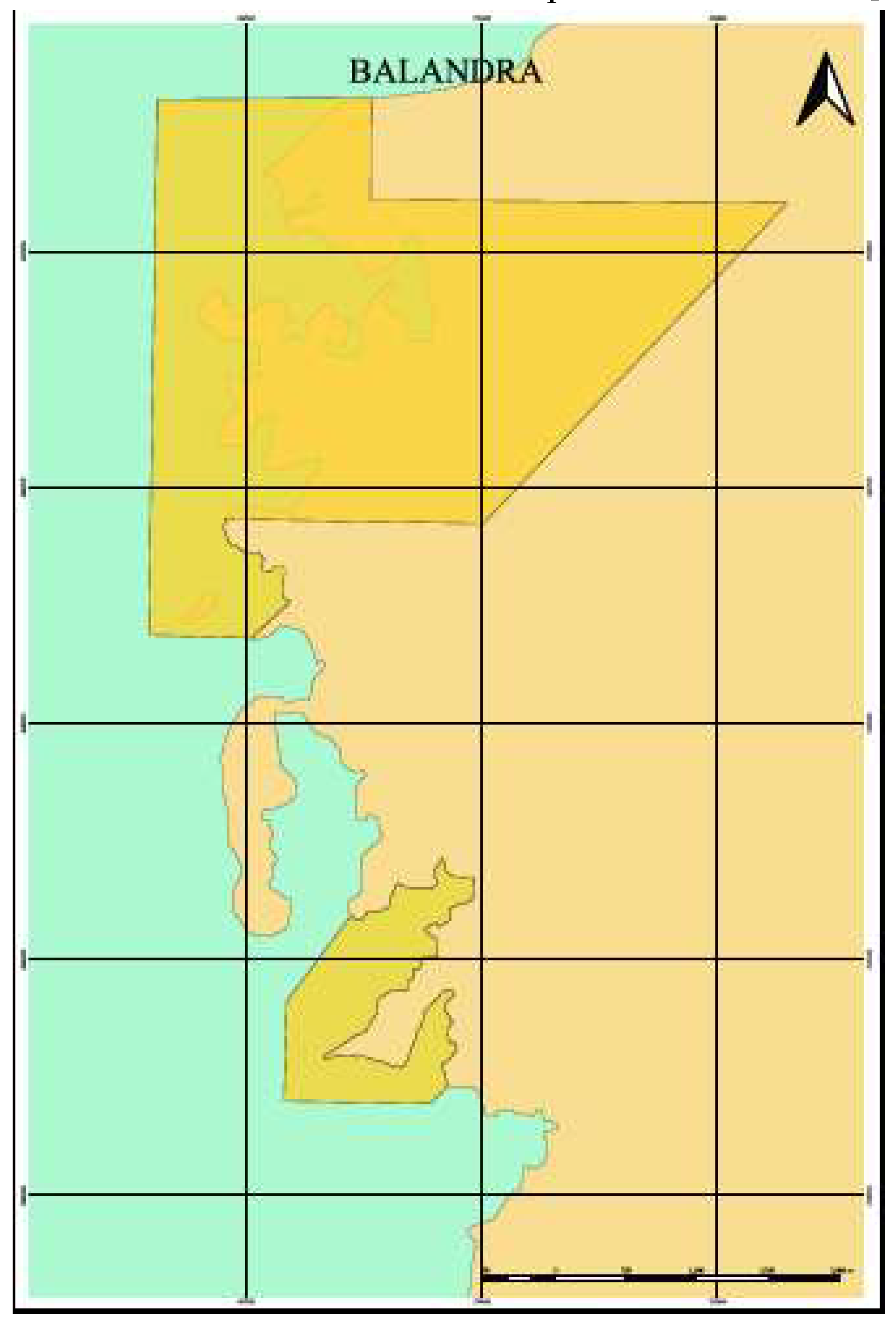
Figure 2.
Histogram: Visits to BNPA since 2017.
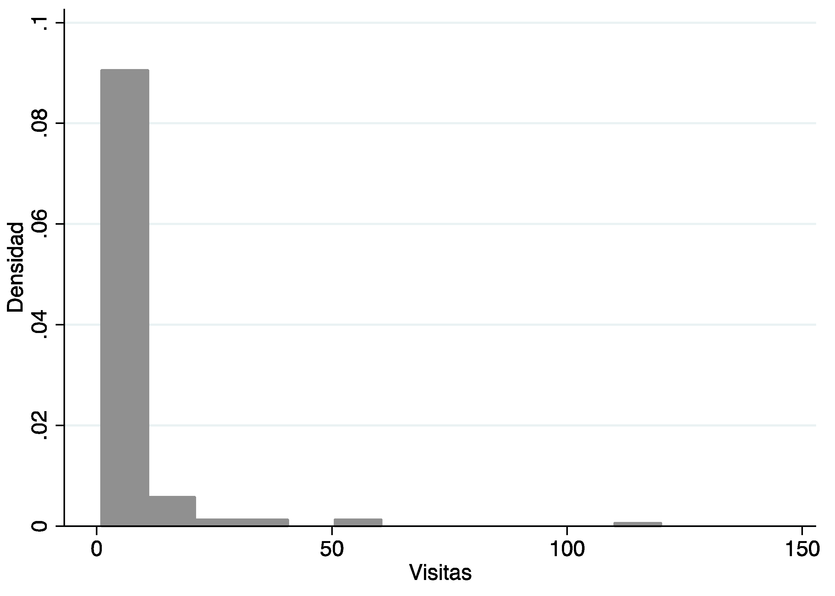

Table 1.
Beaches economic valuation research (US$).
| Author(s)/Year | Country | Site | WTP | Method |
|---|---|---|---|---|
| Zambrano-Monserrate, et al. (2018) [21] | Ecuador | Villamil Beach | 16.95 | ITC |
| Zhang, et al. (2014) [22] | Australia, Queensland | Costa Dorada Beaches | 19.97 | ITC |
| Morales-Zarate, et al. (2019) [23] | México, Baja California Sur | Los Cabos Touristic Corridor | 30.96 | ITC |
| Enriquez-Acevedo, et al. (2016) [24] | Colombia | Caribbean Region | Mín. 3.80 Max. 6.80 |
CV |
| Legget, et al. (2018) [25] |
California, Orange County | Long Beach to Huntington Beach | Mín. 5.78 Max. 20.36 |
ITC |
| Hynes y Greene (2013) [26] |
Ireland | Siverstrand | Min. 11.35 Max. 68.41 |
Panel ITC |
| Voke, et al. (2013) [27] |
United Kingdom | St. David’s, Pembrokeshire | Min. 2.24 Max. 37.56 |
ITC |
|
Source: Self elaboration based on mentioned references. ITC: individual travel cost, VC: contingent valuation | ||||
Table 2.
Variables included in BNPA recreational demand models.
| Variable | Description |
|---|---|
| V | Dependent variable. Number of trips to BNPA in last five years, including actual visit. |
| tc | Travel cost natural logarithm (transportation cost plus cost of the trip or expense made to get to BNPA) |
| first | 1: if is visitor’s first visit to BNPA, 0: no |
| usa | 1: If visitor’s precedence is from USA, 0: Other |
| bnpa | 1: Visiting BNPA or mushroom-shaped stones was their main trip motivation, 0: Other |
| stay | Natural logarithm of staying in La Paz City (days) |
| college | 1: If visitor’s schooling is college, 0: Other |
| income | Natural logarithm of visitor’s declared monthly income |
| pers | Reciprocal of the number of persons traveling with the visitor |
Table 3.
Recreational demand models for BNPA. Dependent: V.
| Variable | P | PT | BN | BNT |
|---|---|---|---|---|
| n=143 | n=143 | n=143 | n=143 | |
| tc | -0.5971 | -0.6479 | -0.2225 | -0.2223 |
| (3.77)*** | (3.67)*** | (3.26)*** | (2.65)*** | |
| first | -1.1118 | -1.1911 | -0.8102 | -1.0314 |
| (5.51)*** | (5.13)*** | (4.91)*** | (4.61)*** | |
| usa | 1.4336 | 1.4975 | 0.9721 | 1.0252 |
| (6.22)*** | (5.97)*** | (5.82)*** | (5.80)*** | |
| bnpa | -0.8206 | -0.8534 | -0.2653 | -0.2092 |
| (3.71)*** | (3.65)*** | (1.83)* | (1.21) | |
| stay | -0.1840 | -0.1727 | -0.1227 | -0.0796 |
| (2.47)** | (2.18)** | (2.27)** | (1.18) | |
| college | 0.7385 | 0.8638 | 0.9702 | 1.4564 |
| (3.51)*** | (3.66)*** | (6.38)*** | (7.26)*** | |
| income | -0.6965 | -0.7378 | -0.5552 | -0.6785 |
| (6.23)*** | (5.99)*** | (6.84)*** | (7.10)*** | |
| pers | -0.6547 | -0.6741 | -0.6449 | -1.0212 |
| (2.01)** | (1.91)* | (2.08)** | (2.37)** | |
| cons | 12.7428 | 13.3188 | 8.2037 | 8.7471 |
| (6.78)*** | (6.37)*** | (9.49)*** | (8.95)*** | |
| ln(α) | -0.8053 | -0.2859 | ||
| (5.74)*** | (2.02)** | |||
| Pearson R2 | 0.8876 | 0.8806 | 0.8723 | 0.8867 |
| Pseudo LL | -625.0543 | -609.8388 | -379.9554 | -356.7948 |
| Chi2 (8) | 170.74 | 169.7 | 173.88 | 148.24 |
| Pr>Chi2 | 0.0000 | 0.0000 | 0.0000 | 0.0000 |
|
Source: Self estimation based on survey data. * p<0.1; ** p<0.05; *** p<0.01 | ||||
Table 4.
WTP, recreational value, and welfare loss for BNPA main beach (US$).
| Concept | Model | |||
|---|---|---|---|---|
| P | TP | NB | TNB | |
| WTP | 3.86 | 3.56 | 10.37 | 10.38 |
| RV-M | 38,996.36 | 35,938.76 | 104,650.45 | 104,744.60 |
| RV-A | 467,945 | 431,255 | 1,255,776 | 1,256,906 |
| VR2021 | 159,430 | 146,929 | 427,845 | 428,230 |
| WL-2MA | 77,993 | 71,878 | 209,301 | 209,489 |
|
Source: Self elaboration Exchange rate: 20.10 MX$/US$ | ||||
Table 5.
Recreational value and welfare loss for BNPA five beaches. Assuming maximum CC (US$).
| Beach | Maximum CC | Model / RV (US$) | ||||
|---|---|---|---|---|---|---|
| Daily | Annual* | P | TP | NB | TNB | |
| Balandra A | 350 | 121,100 | 501,354 | 461,391 | 1,344,210 | 1,345,421 |
| Balandra B | 280 | 96,880 | 401,083 | 369,113 | 1,075,368 | 1,076,337 |
| Frente 1 | 100 | 34,600 | 143,244 | 131,826 | 384,060 | 384,406 |
| Frente 2 | 160 | 55,360 | 229,190 | 210,922 | 614,496 | 615,050 |
| Frente 3 | 94 | 32,524 | 134,649 | 123,916 | 361,016 | 361,342 |
| RV-5BCC | 984 | 340,464 | 1,409,521 | 1,297,168 | 3,779,150 | 3,782,555 |
| WL-5B2M | ---- | ---- | 587,314 | 540,499 | 1,574,682 | 1,576,101 |
|
Source: Based on [57]. *Assuming BNPA opens 346 days a year according with [57]. | ||||||
Disclaimer/Publisher’s Note: The statements, opinions and data contained in all publications are solely those of the individual author(s) and contributor(s) and not of MDPI and/or the editor(s). MDPI and/or the editor(s) disclaim responsibility for any injury to people or property resulting from any ideas, methods, instructions or products referred to in the content. |
© 2024 by the authors. Licensee MDPI, Basel, Switzerland. This article is an open access article distributed under the terms and conditions of the Creative Commons Attribution (CC BY) license (http://creativecommons.org/licenses/by/4.0/).
Copyright: This open access article is published under a Creative Commons CC BY 4.0 license, which permit the free download, distribution, and reuse, provided that the author and preprint are cited in any reuse.


